Munich Personal RePEc Archive
Misspecification and Heterogeneity in
Single-Index, Binary Choice Models
Chen, Pian and Velamuri, Malathi
Victoria University of Wellington
May 2009
Online at
https://mpra.ub.uni-muenchen.de/15722/
Misspecification and Heterogeneity in Single-Index,
Binary Choice Models
By
Pian Chen*
Malathi Velamuri* [email protected]
Abstract: We propose a nonparametric approach for estimating single-index, binary-choice models when parametric models such as Probit and Logit are potentially misspecified. The new approach involves two steps: first, we estimate index coefficients using sliced inverse regression without specifying a parametric probability function a priori; second, we estimate the unknown probability function using kernel regression of the binary choice variable on the single index estimated in the first step. The estimated probability functions for different demographic groups indicate that the conventional dummy variable approach cannot fully capture heterogeneous effects across groups. Using both simulated and labor market data, we demonstrate the merits of this new approach in solving model misspecification and heterogeneity problems.
Keywords: Probit, Logit, Sliced Inverse Regression, categorical variables, treatment heterogeneity
JEL-Codes: C14, C21, C52
* School of Economics and Finance, Victoria University of Wellington, P. O. Box 600, Wellington,
1. Introduction
In this paper, we consider the problem of misspecified binary choice models and model heterogeneity associated with categorical explanatory variables. The leading examples of binary choice models, such as Probit and Logit, are single index models, i.e., Pr(yi =1| )xi =F x( i′β)
i
, where the conditional probability function F is
nonlinear in the single index x′β . The advantage of Probit and Logit specifications over a linear probability model is that the conditional probability function can be restricted to be between zero and one. However, there is no reason to believe that these parametric models necessarily capture the underlying nonlinear pattern in the data generating process. It is well-known that maximum likelihood estimates (MLE) of β are inconsistent if the parametric functional form of (F xi′β) is misspecified.
To consistently estimate index coefficients β, semiparametric methods have been proposed in the literature, including (1) maximum score estimator (Manski 1975, 1985), (2) smoothed maximum score estimator (Horowitz 1992), (3) maximum rank correlation estimator (Han 1987), (4) semiparametric MLE (Klein and Spady 1993), (5) semiparametric least squares (Ichimura 1993), and (6) derivative-based estimator (Powell, Stock, and Stocker 1989).
These semiparametric methods may avoid the model misspecification problem, but they also have technical problems and can be computationally difficult in practice. The first two estimators have convergence rates slower than root-n; the third estimator is root-n consistent and asymptotically normal, but it requires that
( i
F x′β) be monotonically increasing inxi′β . The fourth method estimates the index
coefficients β by maximizing the log likelihood function
where F xˆ ( i′β) is a nonparametric estimate of (F xi′β) and n denotes the sample size.
This estimate attains the semiparametric efficiency bound. But the procedure is time-consuming because it involves estimating (F xi′β) and searching for β iteratively.
The fifth method is also not cheap to compute as it requires solving for (F xi′β) and
( i ) i
F x′β xβ
∂ ∂ ′ for all n. In addition, its asymptotic properties rely on the
assumptions of asymptotic independence and stochastic equicontinuity, which impose restrictions on the nature of data. The last method estimates index coefficients using the density-weighted average derivatives of the regression function. This method is subject to the ‘curse of dimensionality’ because it is based on
1, , i= "
( i ) xi
F x′β
∂ ∂ and the
advantage of the single-index restriction is essentially being lost. A detailed summary of semiparametric estimation of discrete choice models can be found in Pagan and Ullah (1999) and Cameron and Trivedi (2005). For applied researchers, these semiparametric methods are technically demanding and therefore, it is desirable to have a simple and efficient method for estimating single-index, binary-choice models.
We present a new two-step procedure for this purpose. In the first step, we estimate the single-index coefficients β using sliced inverse regression (SIR), a method originally proposed by Li (1991) for dimension reduction. In the second step, we estimate the conditional probability function (F xi′β) using kernel regression of
the binary choice variable yi on the estimated index xi′βˆSIR, where βˆSIR is obtained
from the first step. To differentiate our method from parametric MLE and semiparametric methods, we call it a SIR-Nonparametric method.
function and the error term, thus avoiding model misspecification. Third, the SIR algorithm only requires estimating a covariance matrix and its eigen value decomposition, which is easy to implement and computationally fast. Fourth, the estimated index coefficients,βˆSIR, are root-n consistent, which in turn suggests that
the estimated probability functionF xˆ ( i′βˆSIR) in the second step converges to F x( i′β)
at rate n2/5 by the standard nonparametric regression results.
The two-step SIR-Nonparametric method (i.e.,βˆSIR →Fˆ ) has at least three
comparative advantages. First, we do not estimate β in a traditional maximum likelihood framework whose consistency relies on correct model specification. Second, we do not need to estimate β and F iteratively (i.e., ) as Klein and Spady’s semiparametric MLE (1993), which conserves computational time. Third, it allows us to include a large number of explanatory variables, unlike the derivative-based method of Powell, Stock, and Stocker (1989).
ˆ
MLE
β RFˆ
The second empirical modelling issue we tackle in this paper is how to handle categorical explanatory variables in binary choice models. The common practice is to combine categorical and continuous explanatory variables in a single index (e.g., Horowitz and Härdle 1996). This approach implicitly assumes that the conditional probability functions are identical across groups defined by categorical variables except for horizontal shifts. This assumption may be too strong and rarely satisfied in many empirical data sets.
doing, we can better capture heterogeneous relationships for different demographic groups or geographic regions.
We design four Monte Carlo experiments to show how SIR works compared to parametric MLE and to illustrate model heterogeneity. The first experiment shows that SIR outperforms Probit and Logit MLE when the data generating process is not governed by the Probit or Logit specification. The second experiment indicates that the efficiency loss of SIR to Probit MLE is trivial when the underlying true model is Probit. The third and fourth experiments demonstrate model heterogeneity associated with categorical variables. The results support the sub-sample estimation strategy and again favour SIR to Probit and Logit MLE.
The rest of the paper is organized as follows. In Section 2, we discuss the possible sources of misspecification in binary choice models and motivate our nonparametric approach. Section 3 introduces the SIR theory and estimation algorithm. In Section 4, we compare SIR, Probit and Logit MLE in various settings via Monte Carlo simulations. In Section 5, we demonstrate our modelling strategy for treatment evaluation across heterogeneous demographic groups. Section 6 concludes the paper and suggests directions for future research.
2. Misspecification Problems
To understand the misspecification problems associated with Probit and Logit, we summarize the two models using the following three components: (i) an observable decision variable yi =1⎡⎣y*i >0⎤⎦, where is a continuous latent variable,
*
i
y
[ ]
1⋅ is an indicator function that takes value one if and zero if ; (ii) a
linear latent variable model
*
i
y >0 *
0
i
y ≤
*
i i i
y =x′β ε+ , where xi represents observed covariates and
β is a column vector compatible with xi; (iii) the error term εi is independent of xi.
Assuming ~εi iid N(0,1) generates the Probit model, while εi ~iid standard logistic
distribution generates the Logit model.
The conditional probability function of yi given xi is
(1) pi =Pr(yi =1 )xi =E y x( i i)=F x( i′β).
For the Probit model, F x( i′ = Φ ′β) (xiβ) , where ( )Φ ⋅ is the CDF of the standard
normal distribution. For the Logit model,F x( i′β)=L(xi′β)=exp(xi′β) 1 exp(
[
+ xi′β)]
,estimates (MLE) of β are consistent when the functional form of F x( i′β) is correctly
specified.
However, there are two possible sources of misspecification. First, the model for the latent variable yi* may not be linear in xi′β . Second, the error term εi may not
follow a standard normal or logistic distribution. If the linear latent variable model *
i i
y =x′β ε+ i is correctly specified, quasi-MLE ofβ is consistent as long as the
specified density of εi belongs to the linear exponential family (e.g., Normal,
Exponential, Bernoulli, Poisson). But is unobservable, and therefore it is difficult to check any parametric restrictions imposed on it using empirical data. In this sense, all parametric binary choice models are potentially misspecified. A misspecified parametric model generates not only incorrect parameter estimates but also misleading probability predictions.
*
i
y
To solve this problem, we propose a more general framework as follows: (i) yi =1⎡⎣y*i >0⎤⎦ ; (ii) i
* ( )
i i
y =H x′β +ε , where ( )H ⋅ is unknown; (iii) εi is
independent of xi. We can consistently estimate the index coefficients β using sliced
inverse regression (Li 1991) without imposing parametric structure on H and distributional assumption on
( )⋅
i
ε . We will introduce the theory and estimation
procedure of SIR in Section 3.
The second misspecification problem is the failure of modelling heterogeneity across demographic groups. Suppose that the observed x covariates comprises a set of continuous variables, denoted by x, and a categorical variable, denoted by D
x . For example, D
x could be a marital status dummy variable, with D 1 0
i
be fully captured by a single dummy coefficient α in models likeF x(′ +β αxD)
( )
F x
. In
this model, the difference between the two groups is F x(′β α+ )− ′β , where α represents a horizontal shift of the conditional probability function. This specification restricts the conditional probability function to have the same curvature for the two groups on the entire support of x′β, which may be too strong for many applications.1
We relax this restriction by assuming different nonparametric models for the married and unmarried groups, i.e.,
(2) 1 1 , 1) ( , 1) F x1( i 1)
D D
i i i i i
x x E y x x Pr(
i i
p = y = = = = = ′β
for the married group and
(3) 0 ) 2( )
D
i
F x 2 1 ,i i 0 ( i i, i 0
pi Pr(yi x x ) y x x
D
E = ′β
= =
1( ) F
= =
=
and F2( )⋅ can be different functions; and
for the unmarried group. Here, ⋅ β1 β2
can be different vectors. If we have more than one categorical variable, we can split the sample into several strata and allow a different model for each stratum, i.e.,
(4) pi s=Pr(yi =1 ,x ii ∈s) E(y x ii i, ∈ =s) F xs(i′βs),
=
where s represents the stratum. This generalization enables us to better capture heterogeneous characteristics across different groups.
th
s
In summary, empirical data may have nonlinear conditional probability functions more complicated than those specified in Logit or Probit. This motivates estimating single-index coefficients using nonparametric methods that allow for general functional forms. In the next section, we suggest using sliced inverse regression (SIR) proposed by Li (1991) for this purpose. In addition, categorical
1 In practice, this restriction can be relaxed by interacting the categorical variable(s) with other control
variables may imply different nonlinear models for various demographic groups. Under such a circumstance, splitting data according to categorical variables may be necessary for obtaining consistent estimates of index coefficients. We demonstrate this point in Section 4 via Monte Carlo simulations.
3. Sliced Inverse Regression and Nonparametric Approach
In this section, we briefly introduce the fundamental theory of SIR and outline its estimation procedure. The inverse regression method assumes that the dependence relationship of yi on the K-dimensionalxi is determined only through J linear
combinations of
K
≤
i
x , i.e.,
(5) yi =F x B u( i′ , i),
where B= ⎣⎡β1 " βj " βJ⎤⎦ is K×J and contains J column vectors known as
“effective dimension reduction” (e.d.r.) directions. The regression function F is unknown, x Bi′
i
are called inverse regression variates, and denotes an error term that is independent of
i
u
x and has mean zero. The conditional probability function in (1) is a special case of (5), in whichJ =1 (i.e., single index), yi is a binary variable,
and is an additive error term. ui
Li (1991) proposes using sliced inverse regression of xi on yi to estimate B.
For easy exposition, we standardize xi to
[
]
1/2
(
i X i
z = Σ− x −E xi) , where denotes
the covariance matrix of
X
Σ
K×K xi . Under a linear design condition (Li 1991,
Condition 3.1), Li shows that the centred inverse regression curve is
contained in the linear subspace spanned by
( E zi|yi) 1/2
j X j j 1,2, ,J
η = Σ β ∀ = ⋅
[
⋅⋅ (Li 1991,
degenerate in any direction orthogonal to Span⎡⎣η1 " ηj " ηJ⎤⎦ . Therefore,
1 j J
η η η
⎡⎣ " "
[
⎤⎦ are the eigenvectors associated with the J nonzero eigenvalues
of Cov E z( |i yi)
]
, and the e.d.r. directions are ⎡⎣β1 " βj " βJ⎤⎦ with1/2
1, 2,
j X j j ⋅⋅⋅,J
β = Σ− η ∀ =
.
The eigen decomposition of
[
( |i yi)]
i
z
Cov requires an estimate of .
Li (1991) suggests using the mean values of within several intervals or slices
determined by
E z E z( i|yi)
i
y , which leads to the following SIR algorithm:
Step 1: Standardize xi by an affine transformation to yield
1/2 ˆ ˆi X
−
= Σ ⎡⎣ i−X⎤⎦
z x ,
where ΣˆX and X are the sample covariance and mean of , respectively. xi
Step 2: Divide the range of yi into G slices, denoted by I1,⋅⋅⋅,IG
g
. Let the
proportion of the y si, that fall in slice be wg (g=1, 2, ,⋅⋅⋅ G)
ˆi z
.
ˆ
Step 3: Within each slice, compute the sample mean of , denoted by mg, such
that the sliced mean ˆ 1
( g) yi∈Igzˆi g
m = n w − ∑ .
Step 4: Calculate the weighted variance-covariance matrix of the sliced means
1
ˆ G
g
SIR w m mg ˆ ˆg g′
M = ∑ = , and then find its eigenvalues and eigenvectors.
ˆ
Step 5: Let ηj (j=1, 2, ,⋅⋅⋅ J) be the J largest eigenvectors of MˆSIR. The outputs,
1/2
ˆ ˆ ˆ
j X j
β = Σ− η
, are the estimates of the e.d.r. directions. (j=1, 2, ,⋅⋅⋅ J)
Chen and Li (1998) show that ˆβj from SIR is root-n consistent and
asymptotically normal with a covariance matrix that can be approximated by 1ˆ 1 ˆ ˆ 1
(1 )
j j X
n− λ− −λ Σ− , where ˆλj is the j
th
largest eigenvalue of the matrix in step 4.
The root-n consistency enables us to consistently estimate
ˆ M
( i ) F x
SIR
β
probability function defined in (1), nonparametrically by regressing yi on xi′βˆSIR .
Nonparametric estimates have slower convergence rates than n in general. Consequently, replacing the true β with its root-n consistent estimate does not affect the asymptotic properties of nonparametric estimates (see Chen and Smith 2008).
The remaining task is to determine J, the number of significant e.d.r. directions. To do so, we test the number of zero eigenvalues of . One can use the summation
of the smallest eigenvalues of as the test statistic, i.e.,
ˆ
SIR
M
K− j MˆSIR
1 ˆ
(6) ˆ j K
k j
n λk = + Λ = ∑ ,
where λˆ1≥"≥λˆk ≥"≥λˆK and n is the sample size. Li (1991) derives the asymptotic
distribution for the case where xi is normally distributed. But in many applications, xi may not be normally distributed.
To make inferences for general cases, Cook and Yin (2001, Section 3.3) develop the following permutation test. Let Θ be the K×K eigenvector matrix ofMˆSIR. PartitionΘ = Θ
[
1 Θ2]
, where Θ1 is K× j and Θ2 isK×(K− j). The ideaof the permutation test is that xi′Θ2 should provide no information for given yi xi′Θ1
if H0: j=J is true. If we randomly permute xi′Θ2 and recalculate ˆΛj a large
number of times, we can obtain a permutation distribution of ˆΛj. Comparing the ˆΛj
computed using the original data to its permutation distribution gives the p-value. Specifically, for testing j = 0, 1,⋅⋅⋅, we can use the following procedure:
Step 1: Compute V1i = Θxi′ 1 and V2i = Θxi′ 2.
Step 2: Randomly permute the indices i of V2i = Θxi′ 2 to obtain a permuted set . * 2i
V
Step 3: Construct the test statistic Λˆ*j using the data
*
( ,y xi i), where
* *
1 2i i i
Step 4: Repeat Steps 1-3 several times (e.g., 100 times) and save ˆ*
j
Λ each time.
Step 5: Compute the p-value, which is just the proportion of Λˆ*j’s obtained in Step 4
that exceeds the ˆΛj computed using the original data ( , )y xi i .
We close this section with two remarks on the SIR algorithm and permutation test.2
Remark 1: If yi is a binary variable, the maximum J obtained from SIR is
one. Recall that SIR estimates Cov E z
[
( |i yi)]
using ˆ 1 ˆ ˆG g
SIR g g g
M = ∑ = w m m′
0
whose
maximum rank equals min{G−1,K} because G
g=1w mg ˆg=
∑ , where G is the number
of slices and K is the number of explanatory variables. The binary dependent variable implies that we have only two slices in Step 2 of the SIR algorithm, i.e., G=2. So, SIR based on first-moment information can only identify single-index, binary choice models. To identify more than one index, one needs second-moment based SIR method (Li 1991) or Sliced Average Variance Estimate (Cook and Weisberg 1991).
( |i i) E z y
Remark 2: For single-index models, J is assumed to be one. But it is possible that the single index xi′β may capture little information relevant for yi. If this is true,
J is essentially zero and one should reconsider his selection of explanatory variables. This is similar to a linear regression context where F test suggests that all explanatory variables except the constant term are jointly insignificant. So, the permutation test is still meaningful for single-index models.
In the next section, we demonstrate the misspecification problem and model heterogeneity in single-index, binary choice models via Monte Carlo simulation. The
2 Both GAUSS and STATA codes for the SIR algorithm and permutation test are available upon
focus is on comparing the performance of SIR and parametric MLE in estimating index coefficients under various model settings.
4. Monte Carlo Simulations
We design four Monte Carlo (MC) experiments, each with 1000 replications. The results show that SIR outperforms Logit and Probit MLE when the latent model
is not y x i
*
i = i′β ε+ but is nonlinear in xi′β . But when the Probit model is the true
data generating process (DGP), we show that the efficiency loss of SIR compared to MLE is small given a sample of moderate size. In addition, given the specifications (2)-(3), we find that estimating the misspecified model F x(i′ +β αxiD) with the full sample generates incorrect estimate of β, regardless of whether MLE or SIR is used. We obtain consistent and efficient estimates if we perform SIR for each stratum separately.
4.1 MC Experiment I
We generate n=400 observations using the following DGP. For ,
1, 2, , 400 i= "
(a) xi =
[
x1i x2i x3i x4i x5i]
′ whose five elements are all iid N(0,1);(b) β β(1) β(2) β(3) β(4) β(5)
[
1 0 1 0 0]
′ ′
⎡ ⎤
=⎣ ⎦ = ;
(c) * ( 2)
i i
y = x′β+ 3+εi, whereεi ~iid N(0,1);
(d) yi =1⎡⎣yi* >0⎤⎦.
In this DGP, the latent variable yi* is nonlinear inxi′β , which is one of the
indicate that SIR performs better than Probit and Logit MLE. The estimates of SIR have smaller variances and small-sample biases. Usingβˆ(3), the third element of
[image:15.595.114.482.247.347.2]estimatedβ , as an example, its small-sample biases are 0.05, 0.05, and 0.01 for Probit, Logit, and SIR, respectively; the corresponding standard errors are 0.308, 0.312, and 0.171. 3
Table 1: Probit and Logit MLE v.s. SIR in Experiment I
Methods Estimates βˆ(1) βˆ(2) βˆ(3) βˆ(4) βˆ(5) Probit MLE mean 1.000 0.000 1.050 0.002 -0.007
std. err 0.000 0.205 0.308 0.207 0.210
Logit MLE mean 1.000 0.000 1.050 0.003 -0.008
std. err 0.000 0.208 0.312 0.210 0.212
SIR mean 1.000 -0.002 1.010 -0.001 -0.001
std. err 0.000 0.118 0.171 0.117 0.115
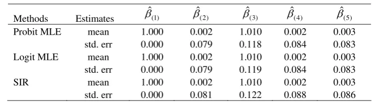
4.2 MC Experiment II
We use the same DGP as in the first experiment except that we change (c) to *
i i
y =x′β+εi, whereεi ~iid N(0,1). In this setting, Probit is the true model, and therefore Probit MLE works best, as indicated by the smallest standard error of 0.118 for βˆ(3) in Table 2. But the efficiency loss of SIR is trivial as the corresponding
standard error is 0.122.
Table 2: Probit and Logit MLE v.s. SIR in Experiment II
Methods Estimates βˆ(1) βˆ(2) βˆ(3) βˆ(4) βˆ(5)
Probit MLE mean 1.000 0.002 1.010 0.002 0.003
std. err 0.000 0.079 0.118 0.084 0.083
Logit MLE mean 1.000 0.002 1.010 0.002 0.003
std. err 0.000 0.079 0.119 0.084 0.083
SIR mean 1.000 0.002 1.010 0.002 0.003
std. err 0.000 0.081 0.122 0.088 0.086
(1)
ˆ
3 In index models, one can only identify parameters up to scale. So, we standardize β to be one and
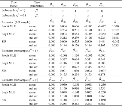
[image:15.595.107.481.576.679.2]4.3 MC Experiment III
We generate n=400 observations using the following DGP.
(a) For i=1, 2,", 400 , xi =
[
x1i x2i x3i x4i x5i]
′ whose elements are all; (0,1) iid N
(b) For the subsample i=1, 2,", 200 , D 1
i
x = and *
1
( 2)
i i
y = x′β + 3+εi
[
0]
, where
1 1(1) 1(2) 1 1 0
β =⎣⎡β β β(3) β1(4) β1(5)⎦⎤′ = 1 0 ′ ;
(c) For the subsample i=201, 202,", 400 , D 0
i
x = and yi*=2 exp(xi′β2)+εi
[
0 1]
, where
2 2(1) 2(2 0
β =⎣⎡β β ) β2(3) β2(4) β2(5)⎦⎤′ = 1 0 − ′
0
;
(d) For i=1, 2,", 400, yi =1⎣⎡yi* > ⎤⎦ and εi ~iid N(0,1).
In this experiment, the categorical variable D i
x implies heterogeneity in the model itself (i.e., different models for the subsample with D 1
i
x = and the subsample
with ). In Table 3, we show that the estimates are far from the true parameters if we naively combine the dummy variable and continuous variables in one index and estimate the single equation
0
D i
x =
( i iD)
F x′ +β αx using the full sample ( ). The estimate of
1, 2, , 400 i= "
α should be around zero, but both Probit and Logit MLE estimates for this parameter are around 3.50 and statistically significant. The SIR method does suggest α =0, but it fails to separately identify the vectors β1 andβ2.
When we split the sample according to the categorical variable and run separate regressions for each subsample, SIR generates estimates with smaller variances and small-sample biases than MLE, as we have seen in the first MC experiment. Note that the signalis much weaker for the subsample with D 0 than
i
for the subsample with D 1, due to the fact that
i
x = E⎣⎡(xi′β1+2)3⎦⎤≈2.5E
[
exp(xi′β2)]
0
D i
x
.
[image:17.595.94.501.195.549.2]This explains why the estimates from the subsample with = have larger standard errors and small-sample biases.
Table 3: Probit and Logit MLE v.s. SIR in Experiment III
True model
True
parameters β(1) β(2) β(3) β(4) β(5)
(subsamplexiD=1) β1 1 0 1 0 0
(subsamplexiD=0) β2 1 0 0 0 -1
Estimates (full sample) βˆ(1) βˆ(2) βˆ(3) βˆ(4) βˆ(5) αˆ Probit MLE mean 1.000 0.004 0.606 -0.005 -0.427 3.520
std. err 0.000 0.204 0.231 0.190 0.212 0.782 Logit MLE mean 1.000 0.004 0.583 -0.005 -0.452 3.490
std. err 0.000 0.212 0.239 0.196 0.224 0.848
SIR mean 1.000 0.000 0.575 0.000 -0.441 -0.042
std. err 0.000 0.144 0.176 0.144 0.167 0.283
Estimates (subsamplexiD=1) 1(1)
ˆ
β βˆ1(2)
1(3)
ˆ
β βˆ1(4)
1(5)
ˆ
β
Probit MLE mean 1.000 -0.008 1.130 -0.002 0.000
std. err 0.000 0.327 0.624 0.311 0.347
Logit MLE mean 1.000 -0.007 1.130 -0.002 0.000
std. err 0.000 0.331 0.627 0.315 0.352
SIR mean 1.000 0.001 1.030 0.002 -0.007
std. err 0.000 0.175 0.254 0.173 0.178
Estimates (subsample D 0)
i
x = βˆ2(1) βˆ2(2) βˆ2(3) βˆ2(4) βˆ2(5) Probit MLE mean 1.000 0.050 -0.035 0.038 -1.250
std. err 0.000 1.160 0.910 0.982 1.750
Logit MLE mean 1.000 0.049 -0.041 0.042 -1.260
std. err 0.000 1.190 1.080 1.040 1.860
SIR mean 1.000 -0.004 -0.013 0.000 -1.050
std. err 0.000 0.255 0.263 0.243 0.387
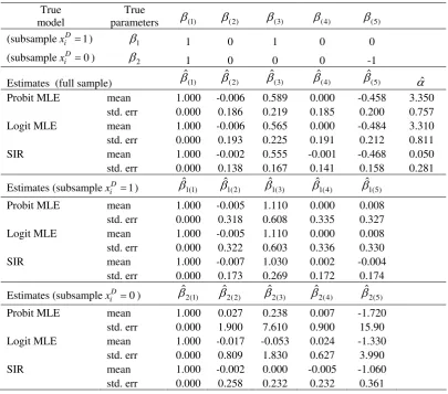
4.4 MC Experiment IV
We use the same DGP as in the third experiment except that the errors are now drawn from a uniform distribution with mean zero and variance one, i.e.,
~ ( 12 2,
i iid unif
ε − 12 2). The non-normal errors make the Probit and Logit
specifications more problematic. In Table 4, Probit and Logit MLE exhibit large standard errors (e.g., 15.90 and 3.99 for βˆ2(5)) in the subsample with (i.e., the
weak signal case).
0
D i
Table 4: Probit and Logit MLE v.s. SIR in Experiment IV
True model
True
parameters β(1) β(2) β(3) β(4) β(5) (subsample D 1)
i
x = β1 1 0 1 0 0
(subsamplexiD=0) β2 1 0 0 0 -1
Estimates (full sample) βˆ(1) βˆ(2) βˆ(3) βˆ(4) βˆ(5) αˆ Probit MLE mean 1.000 -0.006 0.589 0.000 -0.458 3.350
std. err 0.000 0.186 0.219 0.185 0.200 0.757 Logit MLE mean 1.000 -0.006 0.565 0.000 -0.484 3.310
std. err 0.000 0.193 0.225 0.191 0.212 0.811
SIR mean 1.000 -0.002 0.555 -0.001 -0.468 0.050
std. err 0.000 0.138 0.167 0.141 0.158 0.281
Estimates (subsamplexiD=1) 1(1)
ˆ
β βˆ1(2)
1(3)
ˆ
β βˆ1(4)
1(5)
ˆ
β
Probit MLE mean 1.000 -0.005 1.110 0.000 0.008
std. err 0.000 0.318 0.608 0.335 0.327
Logit MLE mean 1.000 -0.005 1.110 0.000 0.008
std. err 0.000 0.322 0.603 0.336 0.330
SIR mean 1.000 -0.007 1.030 0.002 -0.004
std. err 0.000 0.173 0.269 0.172 0.174
Estimates (subsamplexiD =0) 2(1)
ˆ
β βˆ2(2)
2(3)
ˆ
β βˆ2(4)
2(5)
ˆ
β
Probit MLE mean 1.000 0.027 0.238 0.007 -1.720
std. err 0.000 1.900 7.610 0.900 15.90
Logit MLE mean 1.000 -0.017 -0.053 0.024 -1.330
std. err 0.000 0.809 1.830 0.627 3.990
SIR mean 1.000 -0.002 0.000 -0.005 -1.060
std. err 0.000 0.258 0.232 0.232 0.361
This experiment shows that Probit and Logit MLE are very sensitive to incorrect error distribution assumptions when E y( i*| )xi is nonlinear in xi′β , the
sample size is small, and the data is noisy. SIR, however, works well under such circumstances (e.g., a small standard error of 0.361 for βˆ2(5)) because it imposes no
restrictions on the error term εi and the latent model ( *|
i i)
E y x .
researchers. In the next section, we give an example to demonstrate this new estimation method.
5. Application to Treatment Evaluation
There is an extensive literature devoted to evaluating the impact of social programs on program participants. The assignment of individuals to these programs is often non-random as social assistance is generally targeted towards those most in need. For this reason, the difference in average outcomes of participants and non-participants is a biased estimate for the causal impact of program intervention. Various quasi-experimental methods have been proposed to reduce the selection bias due to non-random assignment and recover the true treatment effect. For a detailed overview of these methods, see Heckman et.al. (1998a and 1998b), Cameron and Trivedi (2005), and Imbens and Wooldrige (2008). In this application, we revisit the propensity score matching method, and we compare the estimated propensity scores and treatment effects using the SIR-Nonparametric method, Probit and Logit MLE.
To proceed, we introduce the following notations and definitions. Let
{
m x D ii, ,i i; =1,",n}
be the vector of observations on a scalar-valued outcomevariable m, a vector of observable variables x, and a binary indicator of treatment D. The primary interest of this application is to identify the population average treatment effect on the treated (ATET), defined as
(7) ATET =E m⎣⎡ 1i−m0i Di =1⎤⎦.
Here, and denote the outcomes of an individual i when and , respectively. The ATET can be identified under the ignorability assumption of Rubin (1978)
1i
(8) m0 ⊥D x,
which implies that
(9) ATET =EX
{
E m⎣⎡ 1i−m0i x Di, i =1⎤⎦ Di =1}
=EX
{
E m x D⎣⎡ 1i i, i = −1⎦⎤ E m⎣⎡ 0i x Di, i =0⎦⎤ Di =1}
.The problem is that one cannot observe E m⎡⎣ 0i x Di, i =0⎤⎦ when . One may use
matching methods to approximate
1
i
D =
0i i, i 0
E m⎡⎣ x D = ⎤⎦ based on observable x covariates.
However, if the x covariates are of high dimension, the matching method becomes impractical. Rosenbaum and Rubin (1983) proposed using propensity scores, i.e.,
( ) Pr( 1 )
p x = D= X =x , to facilitate matching under the conditional independence assumption
(10) m m0, 1 ⊥D x,
which in turn implies
(11) m m0, 1 ⊥D p x( ).
Given condition (11), the ATET derived in (9) can be rewritten as
(12) ATET =EX
{
E m p x⎡⎣ 1i ( ),i Di = −1⎤⎦ E m⎡⎣ 0i p x( ),i Di =0⎤⎦ Di =1}
=EX
{
E m⎣⎡ 1i p x( )i ⎤⎦−E m⎣⎡ 0i p x( )i ⎤⎦}
.Matching methods pair program participants with non-participants based on the degree of similarity in the estimated propensity scores. Exact matching, nearest-neighbor matching, kernel matching, and local linear matching are some of the popular matching methods.
(13) q *
1
1 0
{ 1}
T i i i D
ATET n − m m
∈ = ⎡ ⎤
= ∑ ⎣ − ⎦,
where nT denotes the number of treated units being matched with control units and
*
0i
y is the outcome of an untreated unit satisfying * i
(14) i* =
{
j min | ( )p xj −p x( ) |i ∀ ∈j {D=0}}
.The propensity score ( )p x )
is usually estimated using parametric single-index, binary choice models (p x′β , such as Probit and Logit. When these models are
misspecified, βˆMLE is inconsistent and the fitted is an incorrect estimate of
propensity score. As a result, the propensity score matching method may yield biased estimates of the ATET. To demonstrate the advantage of the SIR-Nonparametric method over the conventional parametric methods, we use the National Supported Work (NSW) data on the treatment group and one of the non-experimental control group data sets (PSID-1) constructed by Lalonde (1986) from the Panel Study of Income Dynamics.
ˆ ˆ ( i MLE
p x′β )
4
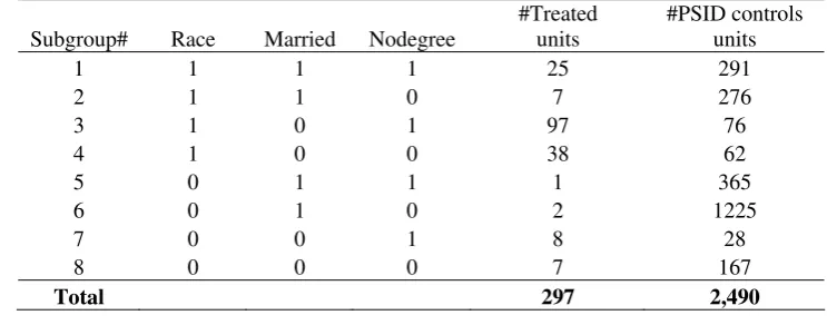
[image:21.595.108.480.550.696.2]First, we divide the data into eight sub-groups based on three dummy variables --- race, marital status and high-school degree status (see Table 5 for details). 5
Table 5: Sub-Groups Based on the Three Dummy Variables
Subgroup# Race Married Nodegree
#Treated units
#PSID controls units
1 1 1 1 25 291
2 1 1 0 7 276
3 1 0 1 97 76
4 1 0 0 38 62
5 0 1 1 1 365
6 0 1 0 2 1225
7 0 0 1 8 28
8 0 0 0 7 167
Total 297 2,490
4 Data are from Rajeev Dehejia’s website http://www.nber.org/~rdehejia/nswdata.html.
5 Race =1 if non-white, 0 if white; Married =1 if married, 0 if single; Nodegree=1 if no high school
For each sub-group, we allow for a different nonparametric propensity score function
(15) pi s =F xs(is′ βs) ∀ ∈i s,
wheres=1, 2,",8 indexes the eight sub-groups and each βs represents a column vector of index coefficients. The observed x comprises four continuous variables --- age, educ, RE74, and RE75. ‘Age’ is defined as age in years in 1974, ‘educ’ measures number of years of schooling in 1974, and ‘RE74’ and ‘RE75’ are real earnings in 1974 and 1975 respectively and measured in thousand of dollars. The earnings refer to the pre-intervention period as the NSW program was administered between 1975 and 1977.
We apply SIR to estimate the index coefficients βs for each sub-group. In
Table 6, we report the estimated index coefficients using SIR as well as those using Probit and Logit MLE. Cook and Yin’s permutation test following the SIR procedure indicates only one significant index for sub-groups 1, 2, 3, 4, 7, and 8 at the 5% significance level. For sub-groups 2 and 5-8, the index coefficients are not estimated precisely because of too few treated units. These sub-groups may be omitted given that they are not important sources of variation in the data. A higher level of aggregation can be applied, requiring the researcher’s discretion.
Among the three methods, SIR is least demanding on model specification and its root-n consistent estimate of index coefficients has more credibility.
Table 6: Estimated Index Coefficients (βˆs) Using the Three Methods
Subgroup# Age Education RE74 RE75 Jointly
significant?
A. Estimates Using SIR Method
1 -0.283 (0.043) 0.621 (0.172) -0.316 (0.080) 0.032 (0.078) Yes 2 -0.056 (0.200) 0.178 (1.190) -0.055 (0.250) -0.196 (0.228) Yes 3 -0.225 (0.021) 0.239 (0.099) -0.074 (0.042) -0.320 (0.050) Yes 4 0.306 (0.029) 0.225 (0.154) -0.086 (0.037) -0.129 (0.034) Yes 5 -0.342 (0.369) -0.326 (2.150) -0.463 (0.539) -0.012 (0.504) No 6 -0.061 (0.779) -0.266 (3.920) 0.047 (0.934) -0.211 (0.938) No 7 -0.067 (0.067) 0.330 (0.398) -0.067 (0.104) -0.513 (0.096) Yes 8 0.153 (0.089) -1.310 (0.369) -0.192 (0.105) -0.049 (0.101) Yes
B. Estimates Using Probit MLE
1 -0.057 (0.018) 0.120 (0.079) -0.234 (0.054) 0.065 (0.041) Yes 2 -0.020 (0.027) -0.006 (0.178) 0.006 (0.025) -0.097 (0.037) Yes 3 -0.041 (0.015) 0.061 (0.069) -0.044 (0.028) -0.196 (0.046) Yes 4 0.097 (0.062) -0.239 (0.218) -0.015 (0.042) -0.382 (0.115) Yes
5 n/a n/a n/a n/a
6 -0.060 (0.050) -0.231 (0.260) -0.029 (0.051) -0.242 (0.222) No
7 n/a n/a n/a n/a 8 -0.017 (0.033) -0.710 (0.330) -0.197 (0.129) -0.032 (0.098) Yes
C. Estimates Using Logit MLE
1 -0.112 (0.035) 0.215 (0.162) -0.487 (0.121) 0.107 (0.094) Yes 2 -0.044 (0.056) -0.008 (0.361) -0.009 (0.059) -0.196 (0.076) Yes 3 -0.068 (0.025) 0.112 (0.121) -0.081 (0.054) -0.332 (0.082) Yes 4 0.168 (0.107) -0.420 (0.38) -0.028 (0.071) -0.643 (0.194) Yes
5 n/a n/a n/a n/a 6 -0.130 (0.108) -0.536 (0.637) -0.067 (0.120) -0.575 (0.525) No
7 n/a n/a n/a n/a 8 -0.045 (0.059) -1.362 (0.701) -0.365 (0.244) -0.058 (0.191) Yes
Note: (i) The numbers in parentheses are the estimated standard errors.
(ii) For sub-groups 5 and 7, MLE fails to generate estimates for Probit and Logit models.
Next, we estimate the propensity score function using kernel regression of the treatment dummy,Di, on the estimated inverse regression variate, xi′βˆs, for i and
. Specifically, we calculate
s ∈
1, 2, ,8 s= "
(16) ˆ ns1
(
1( ˆ ˆ ))
ns1(
1( ˆ ˆ ))
is j i s j s i j i s j s
where i j, ∈s, ns is the sample size of sub-group s, h denotes a bandwidth, and ( )K ⋅
is a user-specified kernel weighting function.
In Figure 1, we plot the estimated propensity score functions. These graphs confirm the two major concerns in this paper. First, parametric specifications may not be adequate for capturing the rich patterns of nonlinearity in the data. Clearly, neither Probit nor Logit specification fit the data well. Both parametric models impose a monotonic relationship between p x(i′β) and xi′β .
)
6
However, the nonparametric propensity score functions suggest that this is not the case for most of the sub-groups.
Second, substantial model heterogeneity exists as indicated by different patterns of p xˆ (i s′∈ βˆs across the eight sub-groups. None of the estimated propensity
score functions of sub-groups 1-7 can be obtained by vertically or horizontally shifting the estimated propensity score function of sub-group 8 (the benchmark with the three dummy variables being zeros). Thus, the common practice of estimating a single equation with pooled data from various socio-economic groups may obscure treatment heterogeneity in the data.
Finally, we calculate the ATET for each sub-group using the estimated propensity scores. The outcome variable is RE78, the real earnings in 1978 (a year after the NSW project was completed) measured in thousand of dollars. Within each sub-group, we calculate the differences in RE78 between individuals in the treatment group and their matched counterparts in the control group. We average these differences to obtain the estimated ATET and report the results in Table 7. We focus on sub-groups 1 (non-white, married, nodegree), 3 (non-white, single, nodegree) and
6 Even some of semiparametric methods have the same monotonicity requirement, such as Han’s
4 (non-white, single, with degree) because too few matched cases in sub-groups 2 and 4-8 may introduce bias to the ATET estimates. 7
Figure 1: Nonparametric Propensity Score Function Using the SIR Variate
7 There are seven matches in group 2, only one match in groups 5-7, and four matches in
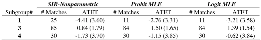
Table 7: Estimates of the ATET Based on the Three Methods
SIR-Nonparametric Probit MLE Logit MLE
Subgroup# # Matches ATET # Matches ATET # Matches ATET
1 25 -4.41 (3.60) 11 -2.76 (3.31) 11 -3.21 (3.58)
3 85 0.84 (1.79) 84 1.50 (1.65) 84 1.39 (1.54)
4 30 -1.73 (3.70) 30 -1.15 (3.85) 30 -0.62 (3.84)
Note: (i) ATET is measured in thousand of dollars;
(ii) The numbers in round brackets are bootstrapped standard errors with 1000 replications.
Clearly, there is substantial treatment heterogeneity across the three groups no matter which method is applied. All three methods suggest that only sub-group 3 benefits from the treatment while sub-groups 1 and 4 worse off after the treatment. The difference between sub-groups 1 and 3 is caused by marriage status, indicating the treatment is more effective on single individuals on average. The difference between subgroups 3 and 4 is caused by education, which implies that the NSW program may have targeted at those without high school degree.
Moreover, the three methods do not result in the same magnitude of estimated ATET. When the ATET is positive (e.g., sub-group 3), the SIR-Nonparametric method suggests a smaller treatment effect than the parametric MLE methods. When the ATET is negative (e.g., sub-groups 1 and 4), the SIR-Nonparametric method suggests a larger negative treatment effect than the parametric MLE methods. These results show that applied researcher should pay attention to model specification as well as heterogeneity when using single-index, binary-choice models.
6. Concluding Remarks
estimates. In addition, we allow for model heterogeneity, which can better capture diverse economic decisions and outcomes across socio-economic groups. Thus, the proposed new method enriches the toolkit for econometric modelling and policy analysis.
References
Cameron, A.C., and Trivedi, P. K., (2005), Microeconometrics: Methods and Applications, Cambridge University Press, New York.
Chen, P., and Smith, A. (2008), “Dimension Reduction Using Inverse Regression and Nonparametric Factors”, mimeo.
Cook, R.D. and Yin, X. (2001), “Dimension Reduction and Visualization in Discriminant Analysis”, Australian & New Zealand Journal of Statistics, Vol. 43(2), pp. 147-199.
Cook, R.D. and Weisberg, S. (1991), Discussion of “Sliced Inverse regression” by K.C. Li, Journal of the American Statistical Association, Vol. 86, pp. 328-332. Dehejia, R. and Wahba, S. (1999), “Causal Effects in Nonexperimental Studies:
Reevaluating the Evaluation of Training Programs”, Journal of the American Statistical Association, Vol.94, No.448, pp.1053-1062.
Drake, C. (1993), “Effects of Misspecification of the Propensity Score on Estimators of Treatment Effect”, Biometrics, Vol. 49, No.4, pp. 1231-1236.
Heckman, J., Ichimura, H., and Todd, P. (1998a), “Matching as an Econometric Evaluation Estimator”, Review of Economic Studies, Vol. 65, No. 2, pp. 261-294.
Heckman, J., Ichimura, H., Smith, J. and Todd, P. (1998b), “Characterizing Selection Bias Using Experimental Data”, Econometrica, Vol. 66, No. 5, pp. 1017-1098. Han, A.K. (1987), “Non-parametric Analysis of a Generalized Regression Model: The
Maximum Rank Correlation Estimator”, Journal of Econometrics, Vol. 35, pp. 303-316.
Horowitz, J.L. (1992), “A Smoothed Maximum Score Estimator for the Binary Response Model”, Econometrica, Vol. 60, pp. 505-531.
Ichimura, H (1993), “Semiparametric Least Squres (SLS) and Weighted SLS Estimation of Single-Index Models”, Journal of Econometrics, Vol. 58, pp. 71-120.
Imbens, G. M., and Wooldridge, J.M. (2008), “Recent Developments in the Econometrics of Program Evaluation”, NBER Working Paper #14251.
Klein, R.W., and Spady R.H. (1993), “An Efficient Semi-Parametric Estimator for Binary Response Models”, Econometrica, Vol. 61, pp. 387-423.
Lalonde, R. (1986), “Evaluating the Econometric Evaluations of Training Programs with Experimental Data”, American Economic Review, Vol. 76, No. 4, pp. 604-620.
Li, K.C. (1991), “Sliced Inverse Regression for Dimension Reduction”, Journal of the American Statistical Association, Vol. 86, pp. 316-333.
Manski, C.F. (1975), “The Maximum Score Estimator of the Stochastic Utility Model of Choice”, Journal of Econometrics, Vol. 3, pp. 205-228.
Manski, C.F. (1985), “Semiparametric Analysis of Discrete Response”, Journal of Econometrics, Vol. 27, pp. 313-333.
Pagan, A. and Ullah, A. (1999), “Nonparametric Econometrics”, Cambridge University Press.
Powell, Stock, and Stocker (1989), “Semiparametric Estimation of Index Coefficients”, Econometrica, Vol. 57, pp. 1403-1430.
Rosenbaum, P. and Rubin, D.B. (1983), “The Central Role of the Propensity Score in Observational Studies for Causal Effects”, Biometrika, Vol.70, No. 1, pp. 41-55.