Development of Numerical Model for Transients in pipe flow for Water
Hammer situation and comparison of different friction equations for
transient friction
Er. Milanjit Bhattacharyya
1, Dr. Mimi Das Saikia
2, Dr. Madan Mohan Das
31 PhD Research Scholar, Deptt. of Civil Engineering, Assam Down Town University, Guwahati, Assam, India 2 Professor, Deptt. of Civil Engineering, Assam Down Town University, Guwahati, Assam, India
3 Formerly, Professor, Deptt. of Civil Engineering, Assam Engineering College, Guwahati, Director of Technical Education Assam, Emeritus Fellow of AICTE, India
---***---Abstract -
Transient flow occurs in pipelines when thepressure and flow rate changes with time. Traditionally, pipe friction during transient events has been modeled using steady friction approximations, such as, the Darcy-Weisbach friction equation. It is then realized that the steady friction approximation produced an insufficient amount of damping as compared to experimental behavior. Numerical model for transients in pipe flow for water hammer situation without the provision of surge tank-for pressure dissipation is developed with MATLAB and different friction equations are compared
with the model.
Key Words: Keywords: Hydraulic pipe transients, friction factor, water hammer, valve, numerical model, discharge, velocity, pressure head etc.
1. INTRODUCTION
Reynold did his pioneering study on the transition between laminar to turbulent state of fluid flow in a cylindrical pipe in 1883. Clearly, surface roughness of the conduit can be a factor for this transition. The logic centers around the friction factor, which influences the pressure/energy losses that occur in a pipe due to friction. One-dimensional quasi-steady model of energy dissipation is in common use. Estimation of loss of energy by the Darcy-Weisbach formula holds good only for slow changes of the velocity field in pipe cross-section. In case of fast changes, like fast transients i.e. water hammer, it fails. Friction and consequential damping in unsteady flow can significantly reduce the harmful effects of some pressure transients and can have a strong influence on behavior close to resonance. Friction losses in pipe conduit accounts for huge time and energy. Accurate determination of friction losses helps in accurate designing of the system – leading to overall safety and economy.
2. LITERATURE REVIEW
The basic unsteady flow equations along a pipe due to closing of the valve near the turbine are non-linear and hence its analytical solution is not possible. Allevi L(1902, 34) [1, 2] developed classical solutions through analytical and graphical methods. Bergeron L(1935,36) [3, 4] also offered graphical solution. Before the advent of computer, graphical solutions mentioned above had been widely used in pipe design.
discharge with time. Ghanbari A. et al(2011) [20] developed a new friction factor correlation with Reynolds Number and relative roughness by means of simple logarithmic and exponential functions. Jinping LI et al (2010)[21] calculated the water hammer by 3D flow simulation in water pipeline system. Urbanowicz K. et al ( 2010) [22] presented a new weighting function as a sum of exponential components in order to enable efficient calculation of the unsteady component wall shear stress. Vitkovsky J.P. et al (2006)[23] tested unsteady friction models and found convolution-based model successful. Urbanowicz K and Zarzycki Z. (2012)[24] modeled unsteady component of wall shear stress as a convolution of local fluid acceleration and as weighing function. Adamkowski A. and Lewandowski M. (2006)[25] analysed unsteady friction models of Zielke, Trikha, Vardy and Brown, Brunone et al and their validation based on own experiment in order to test transient pipe flows in a wide range of Reynold’s number. Pothof I. (2008)[26] proposed and validated a new formulation for the unsteady shear stress against eight transient scenarios in four different systems, conveying water with steady state Reynold’s number varying between 1940 to 1.5 million. Vitkovsky J. et al (2006)[27] presented quantification of the numerical error that occur when using weighting function-based models for the simulation of unsteady friction in pipe transients. Vardy A. et al (2009)[28] presented test results of unsteady skin friction experiments including acceleration, deceleration and acoustic resonance on a large- scale pipeline apparatus for higher Reynold’s number upto 400,000.
3. GOVERNING EQUATION
The flow inside the pipe in case of water hammer situation is unsteady and to analyse the unsteady situation inside the pipe constant friction model cannot be used. Different researchers has proposed different friction models for unsteady analysis. In this study we have considered mainly two friction equations, one is proposed by Barr and the other one is proposed by Chen.
The basic equations of continuity and momentum in unsteady flow along pipe due to closing of the valve near the turbine may be written as:
Continuity: 0 2 x Q gA a t H ………..(1) Momentum: 0 2 1 2
gDA f t Q gA x H …………(2)
Where, H= pressure head, A = area of pipe or conduit, a=velocity of pressure wave, Q= discharge, g= acceleration due to gravity, t = time, f =friction factor, D= diameter of pipe or conduit x = distance along the pipe.
4. METHOD OF CHARACTERISTICS (MOC)
In the MoC the partial differential equations transforms into ordinary differential equations along characteristics line. Equations (1) and (2) are presented as the following finite difference equations for pressure head H and discharge Q,
j
k j k j k j k j k j k j k j k j
k Q Q Q Q
gDA t af Q Q gA a H H
H 1 1 1 1 2 1 1 1 1
1 4 2 2 1
j
k j k j k j k j k j k j k j k j
k Q Q Q Q
gDA t af H H a gA Q Q
Q 1 1 1 1 2 1 1 1 1
1 4 2 2 1
5. BARR’S FRICTION EQUATION
The friction factor f in the above equations is replaced by the following Barr’s explicit approximations which covers full range of flow conditions, from laminar to turbulent.
k D k D R R R Rf e e
e e / 7 . 3 1 / 29 / 1 7 / log 518 . 4 / log 02 . 5 log 2 1 7 . 0 52 . 0 10 10 10 Where,
f = friction factor
k = sand roughness coefficient D = Diameter of pipe
Re = Reynold’s number
6. CHEN’S FRICTION EQUATION
Chen’s friction equation is given by,
8961 . 0 1096 . 1 149 . 7 8257 . 2 / log 0452 . 5 7065 . 3 / log 4 1 e e R D k R D k f Where,f = friction factor
k = sand roughness coefficient D = Diameter of pipe
Re = Reynold’s number
7.ALGORITHM OUTLINE
The comparison of friction values, pressure heads and discharges are done with the use of different friction equations. This is an outline of the algorithm to calculate the pressure head Hi j and the discharge Qi j for the pipe flow hydraulic transient.
[Here ‘i’ refers to the section no. of length along the pipe, ‘j’ refers to the reference no. of the time step]
(Here,
L = Length of the pipe D = Diameter of the pipe H0 = Pressure head at inlet Q0 = Initial discharge a = Velocity of pressure wave g = Acceleration due to gravity
tmax = Time taken for complete valve closure V0 = Initial velocity of the water in the pipe n = No. of sections along the length axis of the pipe m = No. of section along the time axis )
2. Calculate constant values such as A, Av, ∆x, ∆t, xi for i = 1,2,…, n+1, and tj for j = 1,2,…,m+1.
(Here,
A = Cross sectional area of the pipe Av = Cross sectional area of the valve ∆x = Length of each section of the pipe ∆t = Value of each individual time step
3. Create matrices Hij = H(xi,tj), and Qij = Q(xi,tj), and initialize them to zero.
4. Load the initial conditions at time=0, i.e. Qi1 = Qo , and Hi1 =H0
5. Loop on time steps, i.e., for j = 1, 2… m 6. Calculate boundary values Q1 j+1 and H 1 j+1 7. If tj<tmax (valve in process of closing),
8. Use VO(t) = VOo(1-t/tmax) to calculate valve opening. 9. Use CD(t) = CD0(1-t/tmax) to calculate coefficient of discharge at various time steps.
10. Calculate H n+1 j+1
11. If tj ≥ tmax (valve already closed), 12. Make Qn+1 j+1 =0, and Hn+1 j+1 =CP2.
13. Calculate Qi j+1 and H i j+1 at the inner points, i.e., i = 2, 3, …, n. Use left division or inverse matrices to solve the matrix equation.
[image:3.595.312.561.414.535.2]8.IMPLEMENTATION OF NUMERICAL MODEL ON DATA of Saikia M.D. and Sarma A.K.(2006)[19]
Figure 1: Schematic representation of water hammer situation without surge tank.
The numerical model is implemented to the given data of Sakia M.D. and Sarma A.K. (2006)[19]. The pipe is divided into 4 sections of equal length, which means there are 5 locations for the calculations. The lab data are given as follows:-
Length of the pipe, L = 12,000 ft Discharge, Q = 20 ft3/sec
Initial Pressure Head at the different locations: Location 1 (Reservoir end) = 600 ft
Location 2 = 587.5 ft Location 3 = 565 ft Location 4 = 547.5 ft
Location 5 (Valve end) = 530 ft Diameter of pipe, Dt = 2 ft
Area of valve opening = 3.1416 ft2
Surface roughness coefficient, k = 0.007093 ft Kinematic Viscosity, vis = 0.000001 ft2/sec Coefficient of discharge, Cd = 0.90
Velocity of pressure wave, V = 3000 ft/sec
[image:3.595.311.562.595.725.2]Now we have applied all these input conditions to our developed numerical model and the results are plotted as given below:-
Figure 2: Pressure Head v/s time at pipe position, x=5 (from Numerical Model of Saikia M.D. and Sarma A.K.
(2006)[19])
Figure 3: Pressure head vs. time at pipe position, x=5 (Developed Numerical Model using Barr’s friction
[image:3.595.56.279.605.742.2]Figure 4: Discharge v/s time at pipe position, x=4 (from Numerical Model of Saikia M.D. and Sarma A.K.
[image:4.595.314.553.115.240.2](2006)[19])
Figure 5: Discharge v/s time at pipe position =4 (Developed Numerical Model using Barr’s friction
equation using data of Saikia M.D. and Sarma A.K. (2006)[19])
9.FURTHER VERIFICATION OF THE DEVELOPED NUMERICAL MODEL
Now applying the input conditions of Jinping LI, Peng WU and Jiandong YANG (2010)[21] to the developed numerical model as used in the existing water hammer situation for gradual valve closure, the following observations are obtained.
The pipe from the reservoir is divided into 5 sections with 6 nodal points. The nodal points are designated as x=1, x=2, x=3, x=4, x=5, x=6 from the reservoir to the valve end respectively.
The input parameters used in the research paper by LI Jinping are listed below.
Length of the pipe from reservoir to the valve end = 600 m Discharge = 14 m3/s
Pressure Head at the reservoir H = 150 m
Pressure Head at the valve end (i.e. at pipe position x=6) = 140 m
Diameter of pipe = 1 m
Viscosity of water at 15 degree celsius = 1.1386 mm2/s Coefficient of discharge = 0.90
Velocity of pressure wave = 1200 m/s
The developed numerical program is run for 10 seconds and the results are plotted as shown in below.
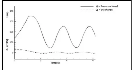
Figure 6: Pressure head v/s time and Discharge v/s time plot at pipe position, x=2 by developed numerical model
using data from Jinping Et Al (2010) [21]
The Pressure head v/s time and Discharge v/s time graph from Jinping et al (2010)[21] is plotted below for comparison.
Figure 7: Pressure vs. time and Discharge vs. time plot at pipe position, x=2 obtained from Jinping Et Al (2010) [21].
Comparing Fig.6 and Fig.7, it is observed that the present numerical model for water hammer simulation in pipe is approximately accurate with the existing results by JI Jinping et al (2010)[21]. Hence the developed model can be used for predicting the pressure and discharge variation in water pipeline system for water hammer situation.
On comparing the graphs, we observe that the numerical model we obtained is quite accurate and thus we can use it to compare different friction model equations. Therefore in this study we have considered the comparison between friction model by Barr’s friction equation and Chen’s friction equation in case of turbulent flow through pipe. The results are plotted below:-
10. COMPARISON BETWEEN TWO FRICTION MODEL: BARR’S FRICTION EQUATION AND CHEN’S FRICTION EQUATION
[image:4.595.321.550.346.467.2]for this study the input parameters are taken from the water hammer problem as discussed on the article No as illustrated in the above analysis.
[image:5.595.323.557.73.196.2]A) The respective output graphs using Barr’s friction equation by the developed numerical model are as shown below:-
Figure 8: Variation in Pressure head, H vs. time (at pipe position x=5) using Barr’s friction equation by Developed
Numerical Model using data from Saikia M.D. and Sarma A.K. (2006)[19]
Figure 9: Discharge at pipe position. x=4 vs. time using Barr’s friction equation by Developed Numerical Model using data from Saikia M.D. and Sarma A.K. (2006)[19]
Figure 10: Friction factor at pipe position, x= 4 vs. time using Barr’s friction equation by Developed Numerical
Model using data from Saikia M.D. and Sarma A.K. (2006)[19]
[image:5.595.49.272.169.289.2]B) The respective output graphs using Chen’s friction equation by the developed numerical model are as shown below:-
Figure 11: Pressure head vs time plot at pipe position x=5 using Chen’s Friction equation by Developed Numerical
[image:5.595.49.275.340.483.2]Model using data from Saikia M.D. and Sarma A.K. (2006)[19]
Figure 12: Discharge vs time plot at pipe position, x=4 using Chen’s Friction equation by Developed Numerical
[image:5.595.325.550.438.578.2]Model using data from Saikia M.D. and Sarma A.K. (2006)[19]
Figure 13: Friction factor vs time plot at pipe position, x= 4 using Chen’s Friction equation by Developed Numerical
Model using data from Saikia M.D. and Sarma A.K. (2006)[19]
11.CONCLUSION
The observations made from the above comparison are:-
[image:5.595.47.276.539.662.2] By comparing the discharge curves, which are calculated from Barr’s friction equation and Chen’s friction equation, we can conclude that both the friction model yields same discharge value. The maximum value of the friction factor calculated
by using Barr’s equation is 0.1274 and the maximum value of the friction factor by using Chen’s equation is 0.0915
Friction factor value (in both the cases of friction calculation) at the initial time ( i.e., at steady state) is 0.0274
The variation of friction factor with respect to time is nearly similar for both the cases (i.e., Barr’s friction equation and Chen’s friction equation). Two friction factor picks are also observed in both
the cases of friction calculation, these picks may arise due to unsteady behaviour of water flow inside the pipe.
REFERENCES:
[1] Allevi L. 1904. Theorie general du movement varie de l’eau dans less tuyaux de conduit. Revue de Mecanique, Paris, France. Vol. 14(Jan-Mar): 10-22 and 230-259.
[2] Allevi L. 1932. Colpo d’ariete e la regolazione delle turbine. Electtrotecnica. Vol. 19, p. 146.
[3] Bergeron L. 1935. Estude ds vvariations de regime dans conduits d’eau:Solution graphique general e. Revue General de l’Hydraulique. Vol. 1, pp. 12 and 69.
[4] Bergeron L. 1936. Estude des coups de beler dans les conduits, nouvel exose’ de la methodegraphique. La Technique Moderne. Vol. 28, pp. 33,75.
[5] Streeter V. L. 1969. Water Hammer Analysis. Journal of Hy. Div. ASCE. Vol. 95, No. 6, November.
[6] Pezzinga G. 1999. Quasi-2D Model for Unsteady Flow in pipe networks. Journal of Hydraulic Engineering, ASCE. Vol. 125(7): 666-685.
[7] Pezzinga G. 2000. Evaluation of Unsteady Flow Resistance by quasi-2D or 1D Models. Journal of Hydraulic Engineering. Vol. l126(10): 778-785.
[8] Watt C.S, Hobbs J.M. and Boldy A.P. 1980. Hydaulic Transients Following Valve Closure. Journal Hy. Div. ASCE. Vol. 106(10): 1627-1640.
[9] Wiggert D. C., Sundquist M. J. 1977. Fixed-Grid Characteristics for Pipeline Transients. Journal of Hy. Div. ASCE. Vol. 103(12): 1403-1416.
[10] Shimada M. and Okushima S. 1984. New Numerical Model and Technique for Water Hammer.Eng. Journal Hy. Div. ASCE. Vol. 110(6): 730-748.
[11] Chudhury M. H.,and Hussaini M. Y. 1985. Second-order accurate explicit finite–difference schemes for water hammer analysis. Journal of fluid Eng. Vol. 107. pp. 523-529.
[12] Zhao M.. and Ghidaoui M. S. 2003. Efficient Quasi-Two dimension Model for Water Hammer Problems. Journal of Hydraulic Engineering, ASCE. Vol. l129 (12): 1007-1013.
[13] Bergant A., Simpson A.R and Vitkovsky J. 2001. Developments in unsteady pipe flow friction modeling. Journal of Hydraulic Research. Vol. 39, No.3 249-257.
[14] Zielke W. 1968. Frequency -dependent Friction in Transient pipe flow. Journal of Basic Eng, ASME. Vol. l 90(9): 109-115.
[15] Brunone B, Golia U.M and Greco M. 1991. Some remarks on the momentum equation for fast transients. Proc. Int. Conf. on Hydraulic transients with water column separation, IAHR, Valencia, Spain. Pp. 201-209.
[16] C.F Colebrook. 1939. Turbulent flow in pipes with particular reference to the region between the smooth and rough pipe laws. J .Ints Civ. Engrs. Vol. 11, pp. 133-156.
[17] Chen NH (1979). An explicit equation for friction factor in pipe. Ind. Eng. Chem. Fundamentals, 18(3): 296.
[18] Barr DIH (1980). Solutions of the Colebrook–While function for resistance to uniform turbulent flow. Proc. Inst. Civil. Eng., Part 271, p. 529.
[19] Saikia M.D. and Sarma A.K. 2006. Simulation of Water Hammer Flows with Unsteady Friction Factor. ARPN Journal of Engg & Applied Sciences, Vol.1, No.4, ISSN 1819-6608.
[20] Ghanbari A., Farshad F. Fred and Rieke H. H. 2011. Newly developed friction factor correlation for pipe flow and flow assurance. Journal of Chemical Engineering and Materials Science Vol. 2(6), pp. 83-86, ISSN-2141-6605.
[21] Jinping LI, Peng WU, and Jiandong YANG. 2010. CFD Numerical Simulation of Water Hammer in Pipeline Based on the Navier-Stokes Equation. V European Conference on Computational Fluid Dynamics. Lisbon, Portugal, 14–17 June 2010.
[22] Urbanowicz K, Zarzycki Z and Kudzma S, Improved Method for Simulating Frictional Losses in Laminar Transient Liquid Pipe Flow, TASK QUARTERLY 14 no 3 (2010):175–188
[23]Vitkovsky, J.P., Bergant, A., Simpson, A.R. and Lambert, M.F. Systematic Evaluation of One-Dimensional Unsteady Friction Models in Simple Pipelines. J. Hyd. Eng. ASCE 132 no.7(2006):696-708.
[25] Adamkowski A and Lewandowski M,Experimental Examination of Unsteady Friction Models for Transient Pipe Flow Simulation, Journal of Fluids Engineering, 128 (2006): 1351-1363
[26]Pothof, I. A turbulent approach to unsteady friction. Journal of Hydraulic Research 46 no.5(2008): 679-690 [27] Vitkovsky, J.P., Bergant, A., Simpson, A.R. and Lambert, M.F. Systematic Evaluation of One-Dimensional Unsteady Friction Models in Simple Pipelines. J. Hyd. Eng. ASCE 132 no.7(2006):696-708.