Techniques of Brain Cancer Detection from MRI using Machine Learning

(1)

TECHNIQUES OF BRAIN CANCER DETECTION FROM MRI USING

MACHINE LEARNING

Aaswad Sawant

#1

_{, Mayur Bhandari}

#2

_{, Ravikumar Yadav}

#3

_{, Rohan Yele}

#4

_{, Sneha Kolhe}

#5

1,2,3,4,5 _{Department of Computer Engineering, Terna Engineering College, Mumbai University, India}

---***---Abstract - Cancer is one of the most harmful disease. To detect cancer MRI (Magnetic Resonance Imaging) of brain is done. Machine learning and image classifier can be used to efficiently detect cancer cells in brain through MRI. This paper is a study on the various techniques we can employ for the detection of cancer. The system can be used as a second decision by surgeons and radiologists to detect brain tumor easily and efficiently.

Key Words: Feature Extraction, MRI, Threshold

Segmentation, Machine Learning, Softmax, Rectified Linear Unit (RELU), Convolution Neural Network (CNN).

1. INTRODUCTION

A brain tumor is a collection, or mass, of abnormal cells in your brain. Human skull, which encloses our brain, is very rigid. Any growth inside such a restricted space can cause problems. Brain tumors can be cancerous (malignant) or noncancerous (benign). When benign or malignant tumors grow, they can cause the pressure inside your skull to increase. This can cause brain damage, and it can be life-threatening.

Brain tumors are categorized as primary or secondary. A primary brain tumor originates in your brain. Many primary brain tumors are benign. A secondary brain tumor, also known as a metastatic brain tumor, occurs when cancer cells spread to your brain from another organ, such as your lung or breast.

Symptoms of brain tumors depend on the location and size of the tumor. Some tumors cause direct damage by invading brain tissue and some tumors cause pressure on the surrounding brain. You’ll have noticeable symptoms when a growing tumor is putting pressure on your brain tissue. If you have an MRI of your head, a special dye can be used to help your doctor detect tumors. An MRI is different from a CT scan because it doesn’t use radiation, and it generally provides much more detailed pictures of the structures of the brain itself.

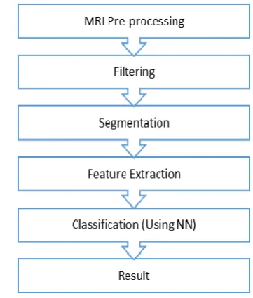
[image:1.595.338.519.188.401.2]

The cancer detection involves the following steps to be performed on the MRI.

Fig -1: Cancer detection Process Flow

1.1 Tensorflow

TensorFlow [8] is an open source software library released in 2015 by Google to make it easier for developers to design, build, and train deep learning models. TensorFlow originated as an internal library that Google developers used to build models in-house, and we expect additional functionality to be added to the open source version as they are tested and vetted in the internal flavour. The name TensorFlow derives from the operations that such neural networks perform on multidimensional data arrays. These arrays are referred to as "tensors". In June 2016, Dean stated that 1,500 repositories on GitHub mentioned TensorFlow, of which only 5 were from Google

Although TensorFlow is only one of several options available to developers, we choose to use it here because of its thoughtful design and ease of use.

(2)

2. LITERATURE SURVEY

2.1 MRI Pre-processing and Filtering

Pre-processing stage removes the noise and also high frequency artifact seen in the image. After these stages the medical image is converted into standard image without noise, film artifacts and labels. There are many methods to perform the above.

2.1.1 Histogram Equalization Technique

The histogram equalization [1] is used to enhance the quality of the image. The continual probability density function and cumulative probability distribution functions are calculated.

The Equation (1) is employed to calculate the cumulative probability distribution function. The frequency of occurrence of every gray value is calculated as well as the image is converted in a more useful form. From the histogram equalization the output image, we can easily notice that the contrast in the image is enhanced. The cumulative probability distribution function emerged by

Fu (u)= ∫ Pu(u)du ….(1)

Here u may be the image pixel value where each pixel carries a continuous probability density function. Pu(u) could be the continuous probability density function, Fu(u) is the cumulative probability distribution function. [1]

2.1.2 Anisotropic Diffusion Filter

Anisotropic diffusion filter [7] is a method for removing noise which is proposed by Persona and Malik. This method is for smoothing the image by preserving needed edges and structures. The purpose of these steps is basically Preprocessing involves removing low-frequency background noise, normalizing the intensity of the individual particles images, removing reflections and masking portions of images. Anisotropic filter is used to remove the background noise and thus preserving the edge points in the image. Diffusion constant which is related to the noise gradient and smoothing the background noise by filtering, so an appropriate threshold value is chosen. A higher diffusion constant value is taken to compare with the absolute value of the noise gradient in its edge.

2.2 Segmentation

Segmentation is a division of the digital image into multiple parts and objective process is to simplify the representation of the image to what is more pronounced for the analysis of the image.

2.2.1 Canny Edge Detection Technique:

The Canny edge detection [2] operator, developed by John F. Canny in 1986, uses a multi-stage algorithm to

detect a wide range of edges and involves the following steps:

• Smooth the image with a Gaussian filter,

• Compute the gradient magnitude and orientation using finite-difference approximations for the partial derivatives, • Apply non-maxima suppression, with the aid of the orientation image, to thin the gradient-magnitude edge image,

• Track along edges starting from any point exceeding a higher threshold as long as the edge point exceeds the lower threshold.

• Apply edge linking to fill small gaps

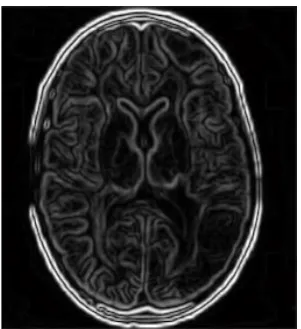
[image:2.595.359.508.304.445.2]

Applying canny edge detection technique to the MRI image in Fig.2, the result is shown in Fig.3.

Fig -2: The original MRI Brain image.

Fig -3: Brain image after applying canny edge detector

2.2.2 Adaptive Threshold Detection Technique:

[image:2.595.359.510.475.640.2]

(3)

method.

2.2.3 Threshold Segmentation:

The threshold [1]of an image is calculated using the Equation (1). The output of the threshold image is a binary image. Thresholding creates binary images from grey-level ones by turning all pixels below some threshold to zero and all pixels above that threshold to 1. If g (x, y) is a threshold version of f (x, y) at some global threshold T, then

g (x , y ) = 1 if f (x , y ) > T

0 if f (x, y) < T (2) f (x , y) is the pixels in the input image and g (x , y ) is the pixels in the output image.

2.3 Feature Extraction:

Feature extraction methods are used to get the most important features in the image to reduce the processing time and complexity in the image analysis.

2.3.1 LOG-Lindeberg Algorithm:

• Read the image.

• Number of blobs detected.

• Calculate Laplacian of Gaussian parameters. • Calculate scale-normalized laplacian operator. • Search of local maxima.

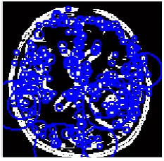
[image:3.595.375.492.286.400.2]

Applying LOG-Lindeberg algorithm to the original MRI Brain image shown in Fig.1 the resulting image is shown in Fig.5.

Fig -5: The feature points of the segmented image are in blue.

2.3.2 Harris-Laplace Technique:

Another method is Harris-Laplace [2]. It relies heavily on both the Harris measure and a Gaussian scale-space representation.

The algorithm follows these steps:

• Find the image parameters. • Scale these parameters. • Find the Harris feature. • Compute the Laplace.

Fig.6 shows the result of applying Harris-Laplace to the segmented image is n in.

Fig -6: The feature points of the segmented image are in blue.

2.4 Classification:

In classification tasks, there are often several candidate feature extraction methods available. The most suitable method can be chosen by training neural networks to perform the required classification task using different input features (derived using different methods). The error in the neural network response to test examples provides an indication of the suitability of the corresponding input features (and thus method used to derive them) to the considered classification task.

2.4.1 SVM Technique:

SVM [7] is one of the classification technique applied on different fields such as face recognition, text categorization, cancer diagnosis, glaucoma diagnosis, microarray gene expression data analysis. SVM utilizes binary classification of brain MR image as normal or tumor affected. SVM divides the given data into decision surface, (i.e. a hyper plane) which divides the data into two classes. The prime objective of SVM is to maximize the margins between two classes of the hyper plane.

[image:3.595.104.219.634.745.2]

(4)

classifier which employs supervised learning to provide better results.

2.4.2 MLP:

In MLP [3], each node is a neuron with a nonlinear activation function. It is based on supervised learning technique. Learning take place by changing connection weights after each piece of data is processed, based on the amount of error in the target output as compared to the expected result. The goal of the learning procedure is to minimize error by improving the current values of the weight associated with each edge. Because of this backward changing process of the weights, model is named as back- propagation.

2.4.3 Naïve Bayes Technique:

Naive bayes [3] is a supervised learning as well as statistical method for classification. It is simple probabilistic classifier based on Bayes theorem. It assumes that the value of a particular feature is unrelated to the presence or absence of any other feature. The prior probability and likelihood are calculated in order to calculate the posterior probability.

The method of maximum posterior probability is used for parameter estimation. This method requires only a small amount of training data to estimate the parameters which are needed for classification. The time taken for training and classification is less.

2.4.4 CNN:

[image:4.595.367.503.165.294.2]

Convolutional Neural Networks (CNNs) [4] have proven to be very successful frameworks for image recognition. In the past few years, variants of CNN models achieve increasingly better performance for object classification. The GOOGLE API Tensoflow [8], makes use of CNN with many layers. Some important layers are listed below.

Fig -7: Structure of CNNs. Nuclear seed maps are fed into 6 layers of artificial neurons: three convolutional layers, two

full-connected layers, and one softmax layer.

2.4.4.1 CONVOLUTION:

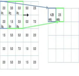
[image:4.595.326.544.495.628.2]

This moving filter, or convolution, applies to a certain neighbourhood of nodes (which may be the input nodes i.e. pixels) as shown below, where the filter applied is 0.5 x the node value.

Fig -8: Convolution

The output of the convolutional mapping is then passed through some form of non-linear activation function, often the rectified linear unit activation function.

2.4.4.2 POOLING:

Again it is a “sliding window” type technique, but in this case, instead of applying weights the pooling applies some sort of statistical function over the values within the window.

[image:4.595.59.270.594.719.2]

Most commonly, the function used is the max () function, so max pooling will take the maximum value within the window.

Fig -9: Pooling

2.4.4.3 RECTIFIED LINEAR UNIT (RELU):

Usually a layer in a neural network has some input, say a vector, and multiplies that by a weight matrix, resulting i.e. again in a vector.

However, most layers in neural networks nowadays involve nonlinearities. Hence an add-on function that, you might say, adds complexity to these output values.

(5)

f(x) = max(0,x)

Therefore it’s not differentiable. The derivative of Relu is very simple.

1 if x > 0, 0 otherwise.

2.4.4.4 SOFTMAX:

[image:5.595.300.570.51.299.2]

Softmax regression is a generalized form of logistic regression which can be used in multi-class classification problems where the classes are mutually exclusive. The Softmax function squashes the outputs of each unit to be between 0 and 1, just like a sigmoid function. But it also divides each output such that the total sum of the outputs is equal to 1.

Fig-10: Softmax

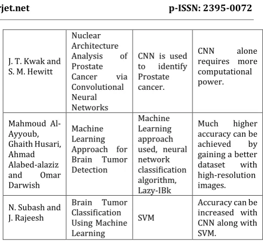
3. COMPARISON TABLE

Table -1: Comparison between Various Papers

Author Paper Title Techniques

Used Observation

Abd El Kader Isselmou, Shuai Zhang, Guizhi Xu

A Novel

Approach for Brain Tumor Detection

Using MRI

Images

Median, High pass filter, Threshold Segmentatio n

Accuracy of

around 95.5%

Ehab F.

Badran, Esraa Galal

Mahmoud, and Nadder Hamdy

An Algorithm for Detecting Brain Tumors in MRI Images

Canny edge detection, Neural Network

used for

classification

The canny edge detection algorithm used

produces the

inaccuracy of 15-16%. Komal

Sharma, Akwinder Kaur , Shruti Gujral

Brain Tumor Detection

based on

Machine Learning Algorithm

MLP and

Naïve Bayes are used.

Accuracy can

probably be

increased by

considering a large data set.

Athiwaratkun, Ben & Kang

Feature Representation in Convolutional Neural Networks

CNN along with SVM is used.

This approach may fail when

dealing with

large dataset.

J. T. Kwak and S. M. Hewitt

Nuclear Architecture

Analysis of

Prostate

Cancer via

Convolutional Neural Networks

CNN is used to identify Prostate cancer.

CNN alone

requires more computational power.

Mahmoud Al-Ayyoub, Ghaith Husari, Ahmad Alabed-alaziz

and Omar

Darwish

Machine Learning Approach for Brain Tumor Detection

Machine Learning approach used, neural network classiﬁcation algorithm, Lazy-IBk

Much higher

accuracy can be

achieved by

gaining a better

dataset with

high-resolution images.

N. Subash and J. Rajeesh

Brain Tumor Classification Using Machine Learning

SVM

Accuracy can be increased with CNN along with SVM.

4. CONCLUSION

Brain tumour diagnosis has become a vital one in medical field because they are caused by abnormal and uncontrolled growing of cells inside the brain. Brain tumour detection is done using MRI and analysing it. The machine learning is very powerful strategy for the detection of the cancer tumour from MRI. A much higher accuracy can be achieved by gaining images taken directly from the MRI scanner. The Tensorflow can be used to tackle the problem of Classification.

REFERENCES

[1] Isselmou, A., Zhang, S. and Xu, G. (2016) A Novel

Approach for Brain Tumor Detection Using MRI Images. Journal of Biomedical Science and Engineering, 9, 44-52.

doi: 10.4236/jbise.2016.910B006.M. Young, The Technical Writer’s Handbook. Mill Valley, CA: University Science, 1989.

[2] E. F. Badran, E. G. Mahmoud and N. Hamdy, "An

algorithm for detecting brain tumors in MRI images," The 2010 International Conference on Computer Engineering & Systems, Cairo, 2010, pp. 368-373.

doi: 10.1109/ICCES.2010.5674887K. Elissa, “Title of paper if known,” unpublished.

[3] Komal Sharma, Akwinder Kaur and Shruti Gujral.

Article: Brain Tumor Detection based on Machine Learning Algorithms. International Journal of Computer Applications 103(1):7-11, October 2014.K. Elissa, “Title of paper if known,” unpublished.

[4] Athiwaratkun, Ben & Kang, Keegan. (2015). Feature

(6)

[5] J. T. Kwak and S. M. Hewitt, "Nuclear Architecture

Analysis of Prostate Cancer via Convolutional Neural Networks," in IEEE Access, vol. 5, pp. 18526-18533, 2017.Athiwaratkun, Ben & Kang, Keegan. (2015). Feature Representation in Convolutional Neural Networks. doi: 10.1109/ACCESS.2017.2747838

[6] Mahmoud Al-Ayyoub, Ghaith Husari, Ahmad

Alabed-alaziz and Omar Darwish, "Machine Learning Approach for Brain Tumor Detection", ICICS '12 Proceedings of the 3rd International Conference on Information and Communication Systems, Article-23, 2012-04-03.

[7] N. Subash and J. Rajeesh, "Brain Tumor Classification

Using Machine Learning" In International Science Press, I J C T A, 8(5), 2015, pp. 2335-2341.

[8] Mart´ın Abadi, Ashish Agarwal, Paul Barham, Eugene