Algorithm for Linear Number Partitioning into Maximum
Number of Subsets
Hussain Md. Mehedul Islam
Department of Computer Science & Engineering, Chittagong University of Engineering & Technology
Chittagong-4349, Bangladesh
Mohammad Obaidur Rahman
Department of Computer Science & Engineering, Chittagong University of Engineering & TechnologyChittagong-4349, Bangladesh
ABSTRACT
The number partitioning problem is to decide whether a given multiset of integers can be partitioned into two "halves" of given cardinalities such that the discrepancy, the absolute value of the difference of their sums is minimized. While Partitioning problem is known to be NP-complete, only few studies have investigated on its variations. Number partitioning problem has a wide range of practical application, like: multiprocessor scheduling, minimization of VLSI circuit size and delay, also used in public key cryptography, message verification, computer password, voting manipulation and bin packing. While lots of investigation have been made for two-way partitioning, only a few for multi-way partitioning, while most of them are not feasible for real time environment. We introduce an improved multi-way partitioning algorithm which is feasible for real time environment. It returns maximum number of subset that can be made based on the order of the numbers as they appear. Maximum number of subset helps us to preempt any process & serve higher priority process with extremely low overhead cost in multiprocessor process scheduling.
Keywords
Anytime algorithm, Greedy heuristic, Linear partitioning, NP-completeness, Partitioning problem.
1.
INTRODUCTION
The Number partitioning problem (Npp) is a NP-Complete problem where the complexity class NP-complete (abbreviated NP-C or NPC) is a class of decision problems.
A decision problem L is NP-complete if it is in the set of NP problems and also in the set of NP-hard problems so that any NP problem can be converted into L by a transformation of the inputs in polynomial time. NP-complete problems are often addressed by using approximation algorithms.
Number Partitioning problem can be defined easily by: Given a list of positive integers & find a
partition, i.e. a subset S such that the discrepancy
S i
i S
i
i
a
a
S
E
(
)
,
is minimized. In the constrained partition problem, the cardinality difference between S and its complement
n
S
S
n
S
m
(
)
2
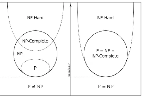
, [image:1.595.311.543.235.392.2]must obey certain constraints. The most common case is the balanced partitioning problem with the constraint |m| ≤ 1.
Fig 1: Euler diagram for P, NP, Complete, and NP-Hard set of problems.
For example, given the integers {8, 7, 6, 5, 4} if we divide them into the subsets {8, 7} and {6, 5, 4}, the sum of the numbers in each subset is 15. This is optimal and known as perfect partition.
Although the partition problem is NP-complete, there is a pseudo-polynomial time dynamic programming solution and a number of heuristics that solve the problem in many instances, either optimally or approximately. For this reason, it has been called “The Easiest Hard Problem” [1].
Now we here by focus on optimal solutions for finding the maximum number of subsets can be made based on the order of the numbers.
It reminds me one of the cherished customs of childhood which needs to choose up sides for a ball game. Where two chief bullies of the neighbourhood would appoint themselves captains of the opposite teams and then they would take turns picking other players. On each round, a captain would choose the most capable (or, toward the end, the least inept) player from the pool of remaining players, until everyone present had been assigned to one side or the other. The aim of this ritual was to produce two evenly matched teams and along the way, to remind each of us of our precise ranking in the neighbourhood pecking order. It usually worked & simply it’s one of the heuristic solutions for number partitioning problem.
There lies a paradox: If computer scientists find the partitioning problem so intractable, how can children over the world solve it every day? Are the kids much smarter?
On the other hand, the success of playground algorithms for partitioning might be a clue that the task is not always as hard as that forbidding term "NP-complete" tends to suggest. As a
matter of fact, finding a hard instance of this famously hard problem can be a hard problem—unless you know where to look. Number partitioning problem is getting importance in both theoretically & practically. It is one of Garey and Johnson’s six basic NP-complete problems that lie at the heart of the theory of NP-completeness [2].
It has a wide range of practical application, like: multiprocessor scheduling, minimization of VLSI circuit size and delay [3], also used in public key cryptography. In fact Number partitioning problem is a problem that actually deals with numbers. In multi-processor scheduling [2] given a set of jobs, each with an associated completion time, and two or more identical processors, assigns each job to a processor to complete all the jobs as soon as possible. Another application of number partitioning is voting manipulation [4].
There are three natural objective functions for number partitioning: 1) minimizing the largest subset sum, 2) maximizing the smallest subset sum, and 3) minimizing the difference between the largest and smallest subset sums. For two-way partitioning, all these objective functions are equivalent, but for multi-way partitioning, no two of them are equivalent [5]. We choose to minimize the largest subset sum & maximizing the number of subsets, which corresponds to minimizing the total time in a scheduling application. Maximum number of subset helps us to pre-empt any process & serve higher priority process with extremely low overhead cost. Minimizing the largest subset sum also allows our number partitioning algorithms to be directly applied to bin packing. Our number-partitioning algorithms keep track of the least subset sum which is the key part of our algorithm. Once we get the least subset sum, we will get the total number of subset & each subset sum, as we are dealing with linear perfect partitioning.
2.
ALGORITHMS AND COMPLEXITY
In view of the NP-hardness of the Npp it is wise to abandon the idea of an exact solution and to ask for an approximate but fast heuristic algorithm. Try a small example. Here are 10 numbers—selected at random from the range between 1 and 10:
2 10 3 8 5 7 9 5 3 2
In this instance, there is 23 ways to divvy up the numbers into two groups with exactly equal sum i.e. perfect partition. Almost any reasonable method will converge on one of these perfect solutions. This is the answer i stumbled onto first:
(2 5 3 10 7) (2 5 3 9 8)
Both subsets sum to 27.
As a matter of fact, among all sets of 10 integers between 1 and 10, more than 99 percent have at least one perfect partition. To be precise, of the 10 billion such sets, 9,989,770,790 can be perfectly partitioned [1].
Maybe larger sets are more challenging?
2.1
Greedy heuristic
A variation on the two - bullies algorithm does just fine. In this approach place the largest number in one of the two subsets. Then continue to place the largest number of the remaining numbers in the subset with the smaller total sum, this continues until all numbers are assigned. The idea behind this greedy heuristics is to keep the discrepancy smaller with every decision. The worst that could happen is that the two subsets are perfectly balanced just before the last number has to be
assigned. This is the motivation for assigning the numbers in decreasing order. The time complexity of the greedy algorithm is given by the time complexity to sort N numbers, i.e. it is
) log
(N N
O . Applied to the set {8, 7, 6, 5, 4} the greedy heuristics misses the perfect solution and yields a partition {8, 5, 4} {7, 6} with discrepancy 4.
2.2
Complete greedy algorithm
Complete Greedy Algorithm (CGA) [6] is an extended version of greedy heuristic. In complete greedy algorithm, sorting the numbers in decreasing order and searching a tree, where each level corresponds to a different number and each branch assigns that number to a different subset. To avoid duplication of any solution that only differs by a permutation of the subset; a number is never assigned to more than one empty subset. We keep track of the largest subset sum in the current best solution, and if the assignment of a number to a subset causes its sum to equal or exceed the current bound, that assignment is pruned. If a perfect partition is found or one in which the largest subset sum equals the largest number, the search returns it immediately. Without a perfect partition, the asymptotic time complexity of CGA is only slightly better than [7], but it has very low overhead per assignment.
2.3
Dynamic programming technique
The problem can be solved using dynamic programming when the size of the set and the size of the sum of the integers in the set are not too big to render the storage requirements infeasible.
This NP-hard instance can be solved by split & merge for about 40 numbers only.
But what if we have n = 500 numbers? Obviously, split & merge does not work anymore. We need some extra information if want to have any hope of solving this in reasonable time. Suppose that we do have some information- we know that the sum of all the numbers is at most N=10000. This little information makes it possible to solve it in
O
(
nN
)
time [8].
In the spirit of dynamic programming, we will create a Boolean array T of size N+1. After the algorithm has finished, T[x] will be true if and only if there is a subset of the numbers that has sum x. Once we have that, we can simply return T[N/2]. If it is true, then there is a subset that adds up to half the total sum.
To build this array, we set every entry to false to start with. Then we set T[0] to true – we can always build 0 by taking an empty set. If we have no numbers in C, then we are done! Otherwise, we pick the first number, C[0]. We can either throw it away or take it into our subset. This means that the new T[] should have T[0] and T[C[0]] set to true. We continue by taking the next element of C.
One important thing is, what if the T[N/2] is not true, we need the closest solution where difference between two set is minimized. For this we need to loop back from N/2 to 0, at first where we get the T[] is true, that is our solution.
Table 1. Dynamic Solution Pseudo Code
bool T[maximum_Sum]; //compute the Total sum n C.size();
Sum 0; for i=0 to n
Sum+=C[i]; //initialize the table T[0]=true; for i=1 to N
T[i] false; //Process each number for i=0 to n
for j = N - C[i] to 0 if(T[j])
T[j+C[i]] true; return T[N/2];
There is another dynamic programming solution for balanced number partitioning problem for a range (0~k) of integers, which cost [9]. This is not even feasible for large number of datasets or multi-ways partitioning (not 2 ways).
2.4
Karmarkar-karp heuristic
The Karmarkar-Karp [10] (KK) heuristic is a polynomial time approximation algorithm for Npp. It applies to any number of subsets, but is simplest for two-way partitioning. It sorts the numbers in decreasing order, and then replaces the two largest numbers in the sorted order by their difference. This is equivalent to separating them in different subsets. This is repeated until only one number is left, which is the difference between the final two subset sums. Adding the difference to the sum of all the numbers, then dividing by two, yields the larger subset sum.
The time complexity of KK heuristic isO(nlog(n)), the space complexity is
O
(
n
)
.This differencing heuristic performs better than the greedy one, but is still bad for instances where the numbers are exponential in the size of the set.
2.5
Korf’s complete anytime algorithm
The KK heuristic is the best known heuristic for two-way partitioning problem. KK heuristic is extended to a complete anytime algorithm [11] that finds better & better solution the longer it is allowed to run, until is finds & proves the optimal solution.
While the KK heuristic separates the two largest numbers in different subsets, the only other option is to assign them to the same subset, by replacing them by their sum. Korf complete anytime algorithm searches a binary tree where the left branch of a node replaces the two largest numbers by their difference and the right branch replaces them by their sum. If the largest number equals or exceeds the sum of the remaining numbers, they are all placed in a separate subset. The first solution found is the KK solution, but anytime algorithm eventually finds and verifies an optimal solution.
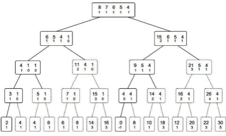
These results in a binary tree, where each node replace the two largest remaining numbers, x1 ≥ x2, the left branch replaces them by their difference, while the right branch replaces them by their sum.
x1, x2, x3….
Iterating both operations (n1) times generates a tree with
) 1 2
( n terminal nodes.
[image:3.595.317.542.195.330.2]Korf’s complete Karmarkar-Karp (CKK) algorithm searches this tree depth-first and from left to right. CKK first returns the largest differencing method (LDM) solution, then continues to find better solutions as time allows.
Fig 2: Tree generated by complete Karmarkar-Karp differencing on the list 8, 7, 6, 5, 4
2.6
New approach for linear partitioning into
maximum subsets
The above all method works for finding two subsets when two subset sums are nearly equal as possible.
But there are many cases where you may need to find the maximum number of subsets possible using minimizing the subset sum.
Now we present our new algorithm which we call Linear Partitioning into Maximum Subsets (LPMS) which meet the above requirement as well, using one criterion - linearity.
Though we use the idea of linear perfect partitioning so the key part is to identify what will be the minimum sum of the subset, once we get the least sum, we just need to iterate through the multiset to subdivide it using this minimum sum to get all other subsets.
Table 2: Function-Partitioning Multiset
Partitioning_Multiset (Multiset[]) size Multiset.length;
for i = 1 to size
Total_Sum Total_Sum + Multiset[i];
Minimum_sumLeastSum(Multiset[],Total_Sum); PrintPartition(Minimum_sum,Multiset[]);
Endfor
The above function finds the total sum of the numbers using a linear loop which cost , where n is the number of integers. Then it call another function named Least Sum which helps to find the minimum sum & finally based on this minimum sum each of the subset will be print out by Print Partition function.
Table 3: Function-Least Sum
LeastSum (Multiset[], Total_Sum) size Multiset.length;
i=0;TempA=0;
while (i<size && (TempA+Multiset[i])<=Total_Sum/2) do
TempA TempA + Multiset[i]; if(Total_Sum MOD TempA == 0)
if(Check_Remaining_Sum(TempA,i+1,size)==true) return TempA;
Endif Endif Endwhile
Return Total_Sum;
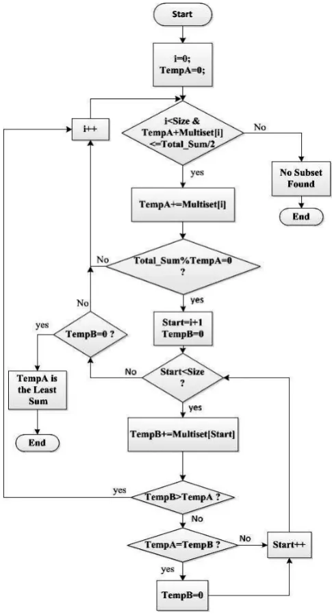
[image:4.595.56.288.77.236.2]Least sum is the key function which serves as the main ingredient of our algorithm. Here we simply sum up to TempA by each of the number from the multiset until we found it as a factor of Total sum. When TempA+ Multiset[i] value is more than half of the total sum then we terminate the loop because at this stage, it is sure that the multiset can’t be partitioned any more. During looping if we find TempA is a factor of total sum than we pass the control to another function named Check Remaining.
Table 4: Function-Check Remaing Check_Remaining_Sum(TempA,Start,size) TempB=0;
for i=Start to size
TempB TempB+Multiset[i]; if(TempB > TempA)
Return 0; else if(TempB = TempA)
TempB=0; Endif
Endfor
if (TempB!=0) Return 0; Endif
Return 1;
The Check Remaining function checks whether the remaining elements of the multiset can form a number of subsets each of having sum TempA. If all the elements can’t form subsets that it goes back to Least sum function to continue sum up to TempA. Otherwise it return with value true to indicate that TempA is our desired minimum sum.
The basic criteria of structured programming that there should be just one entrance & one exit. But our flowchart does not follow it, why? There are some situations where structured programming may need more running time or extra memory in that such cases unstructured programming is favourable to reduce running time or to save wastage of memory.
when we got our final minimum sum then we does not need to go for another iteration that’s why we exit here immediately, which ultimately declare it as an unstructured model of programming but fortunately it reduce our running time.
Fig 3: Flowchart of LPMS for finding minimum sum
The space complexity of our algorithm is and time complexity for best case is , we declare the best case data set as when we get first factor in least sum function is the final desired minimum sum. Where n is the number of elements. Theoretically the worst case complexity of our algorithm is . Theoretically at each stage we can get a factor in Least Sum function and it pass the control to Check Remaining to check whether the remaining element can form subsets, where it iterate the whole array. So final complexity is , which is even better than dynamic programming technique.
3.
EXPERIMENTAL RESULT
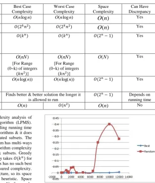
Table 5: Comparative Complexity Analysis
Algorithm Type of Partitioning Best Case Complexity
Worst Case Complexity
Space Complexity
Can Have Discrepancy
Greedy heuristic 2-ways O(nlogn) O(nlogn)
O
(
n
)
YesMulti (k) ways
O
(
n
)
YesComplete greedy algorithm
Multi-ways Yes
Dynamic programming technique
2-ways
O
(
nN
)
[For Range (0~k) of integers
]
)
(
nN
O
[For Range (0~k) of integers]
)
(
N
O
YesKarmarkar karp heuristic
2-ways O(nlog(n)) O(nlog(n)) Yes
Korf’s complete anytime algorithm
2-ways Finds better & better solution the longer it is allowed to run
Depends on running time
LPMS Multi-ways
O
(
n
)
O
(
n
)
NoThe above table shows a comparative complexity analysis of various partitioning algorithms with our algorithm (LPMS). LPMS shows much better performance regarding running time & space complexity comparing with other algorithms & it does not produce any discrepancy among the created subsets. The Greedy heuristic and complete greedy algorithm has multi-ways version for partitioning problem but both algorithm complexity is much higher to partition a multiset into k subsets. Greedy heuristic takes and Complete Greedy takes for partitioning into k subsets and these algorithms has no such best case where it can take less time than its measured complexity. Complete greedy algorithm use tree data structure, so its space complexity is much higher than Greedy heuristic. Space complexity for Complete greedy is & greedy heuristic is . Comparing with these two multi-ways partitioning algorithm, our algorithm (LPMS) is much better considering both time & space complexity. LPMS time & space complexity is much less than these greedy heuristic & complete greedy algorithms. In some cases LPMS is much better than other 2-ways partitioning algorithms. Our algorithm complexity is much better than dynamic solution technique, where DP solution time & space complexity is higher than LPMS. Karmarkar karp heuristic and Korf’s complete anytime algorithm both has 2 ways version whose space complexity is much higher.
So, LPMS is a revolution within the area of partitioning problem algorithm. Where this multi-ways LPMS is better than other multi-ways and in some cases better than others 2-ways algorithms.
We have tested our algorithm on different type of data sets. Following chart based on the run time performance calculation for different types of dataset.
Fig 4: Performance Graph using various data set
4.
CONCLUSIONS
Numerous numbers of researches has been done on two ways number partitioning problem, while very few are on multi-ways partitioning but most of them are not feasible in the real time environment due to their higher complexity. Our algorithm solves this acquaintance with its less complexity than any other algorithm which especially helps for prioritized task scheduling in multi-processor systems, Graph partitioning, VLSI circuit partitioning etc. The challenge involved in using of our Liner partitioning model to solve practical problems stems from the large-scale nature of the model (even though the complexity order of size is of relatively low degree). We believe this challenge may be effectively met however, if the special structure of the model (as developed in this paper) can be exploited judiciously enough, using for example, large-scale optimisation techniques.
Though there is nothing perfect in this world, we are looking for more advance procedures to make this algorithm perfect for other specific applications in the near future, where LPMS solves as a key for any other specific task related to partitioning problem.
The partitioning algorithm proposed here can be used for Breaking Knapsack Cryptosystems as existing partitioning algorithms are used in case. LPMS can also be used to make strong Computer password as many systems still use partitioning algorithm to create system password. Message verification is one of the main applications of number partitioning algorithms; LPMS can be used to make it difficult for the intruder to infer the message without verification. LPMS make Bin packing problem more attractable to researcher. Along with procedural improvement, we want to simulate our algorithm for these applications in a simulated environment. We hope this can help us for vast improvement of all partitioning related algorithm to solve our acquaintance.
5.
REFERENCES
[1] S. Mertens, “The Easiest Hard Problem: Number Partitionin,”A.G. Percus, G. Istrate and C. Moore, eds., Computational Complexity and Statistical Physics (Oxford University Press, New York, 2006), p. 125-139.
[2] Michael R. Garey and David S. Johnson. Computers and Intractability. A Guide to the Theory of NP-Completeness. W.H. Freeman, New York, 1997.
[3] E. Coman and G. S. Lueker, “Probabilistic Analysis of Packing and Partitioning Algorithms,”(John Wiley & Sons, New York, 1991).
[4] Walsh, “Where are the really hard manipulation problems? The phase transition in manipulating the veto rule,” IJCAI-09, p. 324–329.
[5] Richard E. Korf, “Objective functions for multi-way number partitioning,” Symposium on Combinatorial Search (SOCS-10), ATLANTA, GA-2010.
[6] Richard E. Korf, “A complete anytime algorithm for number partitioning,” Artificial Intelligence, paper 106(2), p. 181–203, 1998.
[7] Richard Korf, “A Hybrid Recursive Multi-Way Number Partitioning Algorithm” on Twenty-Second International Joint Conference on Artificial Intelligence, IJCAI, Spain, July 16-22, 2011.
[8] The Wikipedia Website. [Online]. Available: http://en.wikipedia.org/wiki/Partition_problem
[9] The Department of Computing Science - Umeå University
website [online]. Available:
http://www8.cs.umu.se/kurser/TDBAfl/VT06/algorithms/ BOOK/BOOK2/NODE45.HTM
[10] Karmarkar and Karp, “The differencing method of set partitioning,” Technical Report UCB/CSD 82/113, Computer Science Division, University of California, Berkeley, 1982.