Content based Color Image Clustering
Manish Maheshwari
Mahesh Motwani,
PhD.Rajiv Gandhi Technical University,
Bhopal, Madhya Pradesh, India
Sanjay Silakari,
PhD.ABSTRACT
Never before in history has image data been generated at such high volumes as it is today. If images are analyzed properly, they can reveal useful information to the users. Image mining deals with the extraction of implicit knowledge, image data relationship, or other patterns not explicitly stored in the images. Image clustering involves the extraction of features from image databases and then application of data mining algorithm to group images. In this paper a data mining approach to cluster the images using color and texture features are proposed. Three techniques are proposed to extract Color feature, using Color Moments, Block Truncation Coding algorithm and histogram method. To extract texture feature concept of Gray Level Co-occurrence Matrix is extended and applied to color images. K-means clustering algorithm is applied to groups the images.
Keywords
Image Retrieval, Histogram, Color Moments, Gray Level Co-occurrence Matrix, K-Means
1.
INTRODUCTION
The speedy progress in information technology for multimedia system has led to a rapid increase in the use of digital images. A lot of information is available in this data collection that is potentially useful in a variety of applications like crime prevention, military, home entertainment, education, cultural heritage, medical diagnosis, and World Wide Web [1, 2]. How to make use of this information effectively and efficiently is the major challenge. Exploring and analyzing the enormous volume of image data is becoming difficult.
The image database containing raw image data cannot be directly used for retrieval. Raw image data need to be processed and descriptions based on the properties that are inherent in the images themselves are generated. Color and texture are two very important attributes used in image analyses. First order image properties can be successfully determined using color information. Texture generally describes a second order property of surfaces and scenes measured over image intensities.
These inherited properties of the images stored in feature database which is used for retrieval and grouping.
Clustering is a method of grouping data objects into different groups, such that similar data objects belong to the same group and dissimilar data objects to different clusters [3,4]. Image clustering consists of two steps the former is feature extraction and the second part is grouping. For each image in a database, a feature vector capturing certain essential properties of the image is computed and stored in a feature base. Clustering algorithm is applied over this extracted feature to form the group.
In this paper a data mining approach to cluster the images based on color and texture feature is proposed. To extract Color feature three techniques are used separately. Color Moments are used to calculate mean, standard deviation and skewness. A new approach Block Truncation Image Mining (BTIM) is proposed using the concept of Block Truncation Coding to extract color feature. A new histogram quantization algorithm, Histogram Image Mining (HIM) is proposed to calculate 54 color histogram. Gray Level Co-occurrence Matrix is a texture analysis technique has been defined for grayscale images. To extract texture feature we propose a simple extension of these techniques to color images refereed as occurrence Matrix Image Mining (CMIM). The Co-occurrence Matrix of each component of RGB image is calculated and features are extracted. K-means clustering algorithm is applied over these extracted features to form groups of these images.
2.
IMAGE RETRIEVAL
In image retrieval feature extraction is the process of interacting with images and performs extraction of meaningful information of images. The measurements or properties used to classify the objects are called Features, and the types or categories into which they are classified are called classes. Low-level visual features such as color, texture and shape often employed to search relevant images based on the query image. A n-dimensional feature vector represent an image where n is the selected number of extracted features.
Color information is the most widely used features for image retrieval because of its strong correlation with the underlying image objects. A commonly used one is the RGB space because most digital images are acquired and represented in this space However, due to the fact that RGB space is not perceptually uniform, color space such as HSV (Hue, Saturation, and Value), HSL (Hue, Saturation and Luminance), CIE L*u*v* and CIE L*a*b* tend to be more appropriate for calculating color similarities. Color Histogram [1] [5] [6] is the commonly and very popular color feature used in many image retrieval systems. The mathematical foundation and color distribution of images can be characterized by color moments [7]. Color Coherence Vectors (CCV) have been proposed to incorporate spatial information into a color histogram representation [8].
3.
HISTOGRAM
The brightness histogram hf(z) of an image provides the
frequency of the brightness value z in the image- the histogram of an image with L gray-levels are represented by a one dimensional array with L elements. The histogram usually provides the global information about the image. It is invariant to translation and rotation around the viewing axis and varies slowly with changes of view angle, and scale.
which make color depth reduction algorithms a necessity not only for compression but also for image processing. Color image quantization is the process used to reduce the number of colors presented in a digital color image [9] [10].
To define discrete color histograms, quantization of a given color space into a finite number of color cells required. Each of them corresponds to a histogram bin. The color histogram of an image is then constructed by counting the number of pixels that fall in each of these cells. There are many different approaches to color quantization, including vector quantization, clustering, and neural networks [11].
4.
HSV COLOR MODEL
[image:2.595.60.262.308.520.2]Instead of a set of color primaries, the HSV model uses color descriptions that have a more intuitive appeal to a user. To give a color specification, a user selects a spectral color and the amount of white and black that is to be added to obtain different shades, tints and tones. Color parameters in this model are Hue (H), Saturation (S) and Value (V).
Figure 1: HSV Color Model
The 3-D representation of the HSV model is derived from the RGB cube. If we imagine viewing the cube along the diagonal from the white vertex to the origin, we see an outline of the cube that has a hex cone shape as shown in figure 1. The boundary of the hex cone represents the various hues and it is used at the top of the HSV hex cone. In the hex cone, saturation is measured along a horizontal axis and value is along the vertical axis through the center of the hex cone.
Hue is represented as an angle about the vertical axis, ranging from 00 at red through 3600. The vertices of the hexcone are separated by 600 intervals. Yellow is at 600, Green at 1200 and
Cyan opposite red at H=1800. Complementary colors are 1800 apart. Blue at 2400 and Magenta at 3000.
Saturation (S) varies from 0 to 1. It is represented in this model as the ratio of the purity of a selected hue to its maximum purity as S=1. Value V varies from 0 at the apex of the hexcone to 1 at the top. The apex represents black. Conversion of RGB to HSV color model is proposed in [12].
5.
CLUSTERING
There are techniques such as clustering for unsupervised learning or class discovery that attempt to divide data sets into naturally occurring groups without a predetermined class structure. The cluster analysis is a partitioning of data into meaningful subgroups (clusters), which the number of subgroups and other information about their composition or representatives are unknown. Cluster analysis does not use category labels that tag objects with prior identifiers i.e. we don’t have prior information about cluster seeds or representatives. The objective of cluster analysis is simply to find a convenient and valid organization (i.e. group) of the data [3] [4]. Intelligently classifying image by content is an important way to mine valuable information from large image collection. Reference [13] explores the challenges in image grouping into semantically meaningful categories based on low-level visual features. The SemQuery [14] approach proposes a general framework to support content-based image retrieval based on the combination of clustering and querying of the heterogeneous features. Reference [15] describes data mining and statistical analysis of the collections of remotely sensed image. Large images are partitioned into a number of smaller more manageable image tiles. Then those individual image tiles are processed to extract the feature vectors. The concept of fuzzy ID3 decision tree for image retrieval was discussed in [16]. ID3 is a decision tree method based on Shannon’s information theory. Given a sample data set described by a set of attributes and an outcome, ID3 produces a decision tree, which can classify the outcome value based on the values of the given attributes like Color, Texture and Spatial Location. Image dataset were defined in 10 classes (concepts): grass, forest, sky, sea, sand, firework, sunset, flower, tiger and fur. At each level of the ID3 decision tree, the attribute with smallest entropy is selected from those attributes not yet used as the most significant for decision-making.
6.
PROPOSED WORK
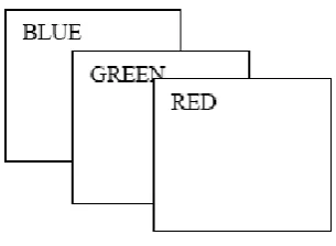
An image is a spatial representation of an object and represented by a matrix of intensity value. It is sampled at points known as pixels and represented by color intensity in the RGB color model. A basic color image could be described as three layered images with each layer as Red, Green and Blue as shown in figure 2.
Figure 2: Image Components
6.1
Color Feature Extraction
6.1.1
Color Moments
[image:2.595.338.491.549.661.2]unique moments (e.g. Normal distributions are differentiated by their mean and variance). It therefore follows that if the color in an image follows a certain probability distribution, the moments of that distribution can then be used as features to identify that image based on color. Stricker and Orengo [7] use three central moments of an image's color distribution in which pkij is the value of the k-th color component of the
ij-image pixel and P is the height of the image, and Q is the width of the image. They are Mean, Standard deviation and Skewness.
MOMENT 1 – Mean:
P Q
E k = 1 ∑ ∑ pkij (1)
PQ i=1 j=1
Mean can be understood as the average color value in the image.
MOMENT 2 - Standard Deviation:
P Q
SDk = SQRT( 1 ∑ ∑ (pkij – E k )2) (2)
PQ i=1 j=1
The standard deviation is the square root of the variance of the distribution.
MOMENT 3 – Skewness:
P Q
Sk = ( 1 ∑ ∑ (pkij – E k )3)1/3 (3)
PQ i=1 j=1
Skewness can be understood as a measure of the degree of asymmetry in the distribution.
6.1.2
Block Truncation Algorithm
A novel algorithm for color feature extraction using Block Truncation Coding (BTC) is proposed. Block Truncation Coding is a compression technique that divides the original image into blocks (typically of size 4× 4 pixels). The intensity value of the block is taken as the mean value of the pixels of the whole block. We extend this concept of block truncation coding technique to multi-spectral images such as color images. The image is divided into its three components red, green and blue, and mean of each component is calculated. Based on this mean value, each component is split into two parts high and low. High is obtained by taking all pixels of that component which are above mean and low is obtained by taking pixels in the image which are below the mean. Concept of color moments is applied over high and low components to construct image features. Steps in Block Truncation Coding Algorithm:
1. Split the image into Red, Green, Blue Components
2. Find the average of each component
Average of Red component
Average of Green component
Average of Blue component
3. Split every component image to obtain RH, RL, GH, GL, BH and BL images
RH is obtained by taking only red component of all pixels in the image which are above red average and RL is obtained by taking only red component of all pixels in the image which
are below red average. Similarly GH, GL, BH and BL can be obtained.
4. Apply color moments to each split component i.e. RH, RL, GH, GL, BH and BL.
5. Apply clustering algorithm to find the clusters.
6.1.3
Color Histogram
6.1.3.1
Rules
for
New
Pixel
Color
Calculation
The hue values range from 0 to 360 degrees and hue represents the dominant color of a pixel. Six symbols are used in order to characterize the hue values at the distance of 60 degrees
Hue = {RED, YELLOW, GREEN, CYAN, BLUE, MAGENTA}
The saturation & value range from 0 to 1.
Saturation = {Small, Medium, Large}
Value = {Small, Medium, Large}
In the proposed work hue, value and saturation values of each pixel are considered as the input for the calculation of the histogram. Using the combination of hue, value and saturation each pixel is converted to 54 colors i.e. 6 quantities of hue, and 3 quantities each of value and saturation are used to form 6 * 3 * 3 = 54. Colors are represented as C1 to C54. Rules for converting each pixel is as follows:
If value is Small
Medium
Large
and saturation is Small Medium
Large
and Hue is
Red Magenta Blue Yellow Cyan
Green
then Color is
C1 C2 C3 : : C54
Thus the image is converted to 54 color image.
6.1.3.2
Histogram
Calculation
Color histogram as a set of bins where each bin denotes the probability of pixels in the image being of a particular color. A color histogram H for a given image is defined as a vector:
H = {H[o], H [1], H [2]…H[c]…H [N]} (4)
Where c represents a color in the color histogram
N is the number of bins in the color histogram, i.e., the number of colors in the adopted color model.
Typically, each pixel in an image will be assigned to a bin of a color histogram of that image, so for the color histogram of an image, the value of each bin is the number of pixels that has the same corresponding color. In order to compare images of different size color histograms should be normalized. The normalized color histogram H' is defined as:
H' = {H'[0], H'[1], H'[2] ...H’[c] ...H’ [N]} (5)
Where H’[c] = H[c]/Max (H[c])
Finally we get a histogram of fifty four colors for each image. A feature database of each image is created by calculating the normalized histogram of these fifty four colors using (5). This feature database acts as input for the clustering algorithm.
6.2
Texture Feature Extraction
Texture is another type of basic low-level image feature that has been used intensively for image retrieval. Texture refers to the presence of a spatial pattern that has some properties of homogeneity [17] [18].
6.2.1
Gray Level Co-occurrence Matrix
Gray Level Co-occurrence Matrix was proposed in [19] [20] by Haralick contains the information about the gray level (intensities) of pixels and their neighbors, at fixed distance and orientation. GLCM depicts how often different combinations of gray level co-occur in an image. The idea is to scan the image and keep track of gray levels of each of two pixels separated within a fixed distance d and direction ө. This spatial relationship can be specified in different ways, the default one is between a pixel and its immediate neighbor to its right. But only one distance and one direction generally are not enough to describe textural features. So, we have used more than one direction and distance.
The Co-occurrence Matrix (Pδ) is created by calculating how
often a pixel with Gray-level I occurs in a specific spatial relationship (distance and direction) to a pixel with Gray-level j. In order to estimate the similarity between different gray level co-occurrence matrices, Harlic proposed 14 statistical features extracted from them. To reduce the computational complexity, only some of these features were selected. The description of 4 most relevant features that are widely used –
1) Contrast returns a measure of the intensity contrast between a pixel and its neighbor over the whole image.
∑ ∑ (i - j)2 Pδ (i,j) (6)
i j
2) Correlation returns a measure of image linearity, how correlated a pixel is to its neighbor over the whole image.
∑ ∑ (i - μi ) (j – μj ) Pδ (i,j) (7)
i j σi σj
3) Energy Returns the sum of squared elements in the GLCM.
∑ ∑ P2
δ (i,j) (8)
i j
4) Homogeneity Returns a value that measures the closeness of the distribution of elements in the GLCM to the GLCM diagonal
∑ ∑ Pδ ( i , j ) (9)
i j 1+ | i – j |
Where Pδ (i,j) is the co-occurrence Matrix under a specific
condition δ (ө, d ), in which d denotes the distance and ө is the orientation between two adjacent intensity (i,j). μi and μi are
means , σi and σj are the standard deviations
6.3
K-Means Clustering Algorithm
K-means is one of the simplest unsupervised learning algorithms in which each point is assigned to only one particular cluster. The procedure follows a simple, easy and iterative way to classify a given data set through a certain number of clusters (assume k clusters) fixed a priori. The procedure consists of the following steps:
Step 1: Set the number of cluster k
Step 2: Determine the centroid coordinates
Step 3: Determine the distance of each object to the centroids
Step 4: Group the object based on minimum distance
Step 5: Continue from step 2, until convergence that is no object move from one group to another.
7.
EXPERIMENTS
The proposed scheme has been performed using an image database of 1000 images including 10 classes, which is
downloaded from the website
http://wang.ist.psu.edu/iwang/test1.tar. Each class has 100 images. Each image is of size 384*256 or 256*384 pixels. The system is developed in Matlab.
To assess cluster performance two statistical measures Recall and Precision are calculated for each class.
Recall is the proportion of obtained images that have been retrieved among all the relevant images in the database.
Recall = Number of Relevant Images Retrieved Total Number of Relevant Images
Precision is the proportion of relevant images among the retrieved images.
Precision = Number of Relevant Images Retrieved Total Retrieved Images
7.1
Experiment using Color Moments
The first experiment computes color moments for each of the three color components RGB. Each color component yields a feature vector of three elements i.e. mean, standard deviation and skewness. Thus total nine feature vectors are calculated for one image and stored in feature database. The k-means clustering algorithm is applied over this feature database. Table 1 show Recall and Table 2 show Precision of each class to evaluate the performance.7.2
Experiment using BTC
7.3
Experiment using Color Histogram (54
colors)
[image:5.595.316.554.72.237.2]In this experiment convert image from RGB to HSV color space. Using HSV values, convert pixel values to C1 to C54. Count C1 to C54 for each Image to calculate 54 color histogram. Thus total 54 feature vectors are calculated for one image and stored in feature database. The k-means clustering algorithm is applied over this feature database. This technique is referred as Histogram Image Mining (HIM). For each class Recall and Precision are calculated to evaluate the performance as indicated in Table 1 and Table 2 respectively..
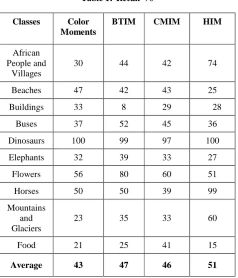
Table 1:Recall
%
7.4
Experiment using Color Moments and
GLCM
In this experiment composite feature of the moment and GLCM is obtained. First compute color moments for each of the three color components. Each color component yields a feature vector of three elements mean (E), standard deviation (SD) and skewness (S).
Next apply the concept of Gray Level Co-occurrence Matrix to form a co-occurrence matrix (Pδ). For every value of
distance d, orientation ө is considered. We are taking four distances and four orientations to obtain Pδ. Thus 16
co-occurrence matrices are obtained for each color component as follows:
Pδ(ө, d ) = { P0,1, P0,2, P0,3, P0,4, P45,1, P45,2, P45,3, P45,4, P90,1,
P90,2, P90,3, P90,4, P135,1, P135,2, P135,3, P135,4} for 4 distance d
(i.e. 1,2,3,4) and 4 orientation ө (i.e. 00
,450,900,1350 degrees). Thus 16 Pδ is obtained.
Calculate four features- Contrast, Correlation, Energy and Homogeneity for each co-occurrence matrix Pδ obtained
above.
As there are 16 co-occurrence matrices Pδ and 4 features are
calculated for each Pδ, feature vector of 16 * 4 =64 elements is
obtained for each color component.
Figure 3: Average Recall
[image:5.595.49.288.208.487.2]Thus total 67 elements (3 color moments + 64 Co-occurrence features) feature vector is generated for each color component red, green and blue respectively. Obtain feature matrix of each image by combining feature vector of each component above. Thus total 67 * 3 = 201 feature vectors are calculated for one image. Store feature vector of each image in the matrix and apply k-means clustering algorithm to groups. This technique is referred as Co-occurrence Matrix Image Mining (CMIM). Calculate Recall and Precision to evaluate the performance.
Table 2: Precision %
Classes Color
Moments BTIM CMIM HIM
African People and
Villages
25.43 33.58 27.81 41
Beaches 40.17 42.42 51.81 42
Buildings 23.57 7.92 47.5 32
Buses 35.24 44.83 50.56 51
Dinosaurs 92.59 97.06 97.97 84
Elephants 35.56 44.83 27.5 40
Flowers 90.32 94.12 90.91 77
Horses 54.95 58.82 59.1 78
Mountains and Glaciers
34.33 43.21 29.46 39
Food 20.79 22.32 26.97 23
Average 45 49 51 51
Figure 3 shows the average recall value of various methods in pictorial form. It shows that average recall value for HIM is highest.
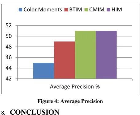
Figure 4 shows the average precision value of various methods. It shows that average precision value for HIM and the average precision value for CMIM is equal and highest.
0 10 20 30 40 50 60
Average Recall %
Color Moments BTIM
Classes Color Moments
BTIM CMIM HIM
African People and
Villages
30 44 42 74
Beaches 47 42 43 25
Buildings 33 8 29 28
Buses 37 52 45 36
Dinosaurs 100 99 97 100
Elephants 32 39 33 27
Flowers 56 80 60 51
Horses 50 50 39 99
Mountains and Glaciers
23 35 33 60
Food 21 25 41 15
[image:5.595.313.561.359.649.2]Figure 4: Average Precision
8.
CONCLUSION
Image clustering consist of two steps: one is the extraction of features from images and another is the application of clustering algorithm over these extracted features to group images. The image is composed of pixels of red, green and blue values. In the proposed work image is divided into three components and color and texture features are extracted over these components. A new color feature extraction method based on BTC which is used for compression is developed. A new color histogram technique, which is quantized to 54 colors, is proposed. Co-occurrence Matrix which is used for Gray Level images is extended to extract texture feature of color images. These obtained features are applied to K-means clustering algorithm to groups the images. The results of these feature extraction methods are compared which are encouraging.
9.
REFERENCES
[1] H.J.Zhang et al., “Video Parsing, Retrieval and Browsing: an Integrated and Content-Based Solution”, Proc. ACM Multimedia 95, San Francisco, Nov 95
[2] B. Furht, S.w.Smoliar, and H.J.Zhang, “Image and Video Processing in Multimedia systems, Kluwer Academic Publishers, Norwell MA, 1995
[3] J. Han and M.Kamber, “Data Mining concepts and Techniques”, Morgan Kaufmann Publishers, 2010
[4] A.K.Pujari, “Data Mining Techniques”, University Press, 2009
[5] Wayne Niblack, Ron Barber, William Equitz, Myron Flickner, Eduardo H. Glasman, Dragutin Petkovic, Peter Yanker, Christos Faloutsos, Gabriel Taubin: “The QBIC Project: Querying Images by Content, Using Color, Texture, and Shape”, Storage and Retrieval for Image and Video Databases (SPIE) 1993, pp 173-187
[6] Alex Pentland, Rosalind W. Picard, Stan Sclaroff, “Photobook: Tools for Content-Based Manipulation of Image Databases”, Storage and Retrieval for Image and Video Databases (SPIE) 1994, pp 34-47
[7] M.Stricker and M.Orengo, “Similarity of color images”, Storage and Retrieval for Image and Video Databases III (SPIE) 1995, pp 381-392
[8] Greg Pass, Ramin Zabih, Justin Miller: Comparing Images Using Color Coherence Vectors. ACM Multimedia 1996, pp 65-73
[9] Yuchou Chang, Dah-Jye Lee1, Yi Hong, James Archibald, and Dong Liang, "A Robust Color Image Quantization Algorithm Based on Knowledge Reuse of K-Means Clustering Ensemble", Journal of Multimedia, Vol. 3, No. 2, June 2008, pp 20-27
[10]Mahamed G. Omran, Ayed Salman and Andries P. Engelbrecht, "A Color Image Quantization Algorithm Based on Particle Swarm Optimization", Informatica 29, 2005, pp 261–269
[11]H.J. Zhang and D. Zhong, “A Scheme for visual feature-based image indexing”, Proceedings of SPIE conference on storage and retrieval for image and video databases III, 1995, pp36-46
[12]Wei-Ying Ma and H. Zhang, “Content Based Image Indexing and Retrieval”, Handbook of Multimedia Computing CRC Press, 1999, pp 227-254
[13]Y. Uehara, S. Endo, S. Shiitani, D. Masumoto, and S. Nagata, ”A computer-aided Visual Exploration System for Knowledge Discovery from Images”, In Proceedings of the Second International Workshop on Multimedia Data Mining (MDM/KDD'2001), San Francisco, CA, USA, August, 2001.
[14]Gholamhosein Sheikholeslami, Wendy Chang, Aidong Zhang, “SemQuery: Semantic Clustering and Querying on Heterogeneous Features for Visual Data”, IEEE Trans. Knowledge and Data Eng. 14(5), 2002, 988-1002,
[15]Krzysztof Koperski, Giovanni Marchisio, Selim Aksoy, and Carsten Tusk, "Applications of Terrain and Sensor Data Fusion in Image Mining", IEEE 2002, pp 1026-1028
[16]Ying Liu1, Dengsheng Zhang1, Guojun Lu1 , Wei-Ying Ma2, "Deriving High-Level Concepts Using Fuzzy-Id3 Decision Tree for Image Retrieval”, IEEE 2005, pp 501-504
[17]Jiji G. Wiselin, Ganesan L., Ganesh S. Sankar, "Unsupervised Texture Classification", Journal of Theoretical and Applied Information Technology, pp 373-381, 2005 - 2009
[18]Saroj A. Shambharkar, Shubhangi C. Tirpude, "A Comparative Study on Retrieved Images by Content Based Image Retrieval System based on Binary Tree, Color, Texture and Canny Edge Detection Approach", IJACSA Special Issue on Selected Papers from International Conference & Workshop On Emerging Trends In Technology, pp 47-51, 2012
[19]Haralick, R.M., Shanmugam, K., Dinstein, I.: Textural features for image classification. IEEE Transactions on Systems, Man and Cybernetics 3, 1973, pp 610-621
[20]Haralick, R.M. Statistical and structural Approaches to Texture, Proceedings of IEEE, 1979, pp786- 804.
42 44 46 48 50 52
Average Precision %