Error Minimization in Localization of Wireless Sensor Networks using Genetic Algorithm

Error Minimization in Localization of Wireless Sensor

Networks using Genetic Algorithm

Sivakumar.S

Asst. Professor Department of Information

Technology

PSG College of Technology Coimbatore, India

R. Venkatesan

Professor Department of Computer

Science & Engineering PSG College of Technology

Coimbatore, India

Karthiga.M

Student

Department of Computer Science & Engineering PSG College of Technology,

Coimbatore, India

ABSTRACT

The important tasks in a wireless sensor network such as routing, target tracking are highly dependent on the location of a sensor node. Hence localization becomes an essential criterion in wireless sensor networks. Higher the localization accuracy better is the performance of the sensor network as a whole. Traditional mathematical algorithms can be used for localization. But these algorithms do not give very high localization accuracy. Genetic algorithm is proven to be effective in searching a solution space and hence can be modeled for the localization problem in Wireless Sensor Network (WSN). The strategy used in this paper for localization uses two phases. The first phase uses a traditional range free localization algorithm based on Mobile anchor to estimate the location of a sensor node roughly. The second phase is a post optimization phase that uses Genetic algorithm which increases the accuracy of localization.

General Terms

Localization in Wireless Sensor Networks.

Keywords

Wireless sensor networks, localization, mobile anchor, post optimization, genetic algorithm.

1.

INTRODUCTION

A wireless sensor network is a self-organized, multi-hop network consisting of a large number of small sensor nodes. WSN is useful in monitoring many environmental conditions like temperature, pressure etc. Each sensor node has the capacity to sense, process, communicate and transmit the sensed data [1]. All the nodes collaboratively work together and transmit the sensed data to the remote site via the satellite or the internet. Localization of the sensor nodes is crucial in WSN as in many applications the measured data is meaningless without the location information [2].

Localization is the process of making each sensor node in the sensor network, aware of its geographic position. The simplest solution is attaching a GPS (Global Positioning System) to each sensor node. But this solution is costly provided when the sensor nodes are large in number. Moreover it makes the sensor node bulkier [3]. Hence many algorithms exists which are used to localize the nodes. Basic principle behind each of these algorithms is the same. They have a few nodes among all the sensor nodes, which know their location precisely in advance (hardcoded or fit with a GPS).

Algorithms use such nodes (Anchor nodes) to localize other sensor nodes [4]. Broadly any localization algorithm falls in one of the following two categories. They are range based and range free algorithms.

Range based algorithms use some hardware for localization whereas range free methods use the messages passed among the sensor nodes for localization. Range based algorithms use absolute distance estimation or angle estimation between two nodes for localization. Some of the range based algorithms are Angle of Arrival (AOA) [5], Time of Arrival (TOA) [6], Time Difference of Arrival (TDOA) [7], and Received Signal Strength Indicator (RSSI) [8]. Range based methods give fine grained accuracy but the hardware used for such methods are expensive. The limitations in terms of cost prevent the use of range based methods.

Range free methods use the content of messages from anchor nodes and other nodes to estimate the location of non anchor sensor nodes. Distance Vector Hop (DV-Hop) method [9], Centroid Algorithm [10] are few range-free algorithms. Range free algorithms sometimes use mobile anchors for localization [11]. Range free algorithms are not costly, but they provide coarse grained accuracy.

The proposed localization approach, called Localization with Mobile Anchors and Genetic Algorithm (LMA-GA) can be visualized to work in two phases. The first phase uses a range-free approach, where the anchor nodes are mobile. Second phase is an optimization phase using Genetic Algorithm as the optimization strategy.

The rest of the paper illustrates the related research works in this area, elaborates the proposed LMA-GA algorithm and compares the performance of LMA-GA with an existing algorithm namely Mobile Anchor Positioning (MAP).

2.

RELATED WORK

In [12] Kuo-Feng Ssu et al. has presented a range free algorithm which uses the conjecture that a perpendicular bisector of a chord passes through the centre of the circle. When there are two such chords of the same circle, their perpendicular bisectors will intersect at the centre of the circle.

A mobile anchor moves around the sensor field passing its location as messages. Assuming that the sensor node is the centre of a circle, it collects mobile anchors location at various points.

Extreme points can be assumed as location of the anchor when it enters and leaves the sensor node‟s communication range. They act as the chord‟s end points. Two such pairs of endpoints are chosen (two chords). Their intersection point is the center of the circle or the sensor node‟s location.

sensor nodes. A sensor node selects four beacons among all collected beacons. The first group (two beacons) is the location of the mobile anchor node when it firstly enters the communication range of the sensor node. The second group is the location of the mobile anchor node when it secondly enters the communication range of the sensor node.

After these positions and the communication range are obtained, four circles are constructed with the chosen four points as centers. Four intersection points s1, s2, s3, s4 of the

circles are calculated. Then using the centroid formula on the four intersection points, the position of the sensor node is calculated.

In [14] W-H Liao et al. has proposed an algorithm (MAP) in which each sensor node receives all beacons in its receiving range from the moving anchor as the anchor moves around the sensing field.

The sensor node selects the farthest two beacons from the received beacons. The node constructs two circles with each chosen beacon as centre. The radius of the circle is the communication range of the sensor node. It determines the intersection points of the two circles. Out of the two points one is chosen to be the location of the sensor node based on a decision strategy.

In [15] Wenwen Li et al. has proposed the Genetic algorithm for localization of the sensor nodes and has constructed the solution space, coded the solutions, formulated the fitness function, used selection mechanism to choose the parents for the next generation, used reproduction on the individuals, and obtained the solution with high accuracy.

The last approach (genetic algorithm) gives good localization accuracy. But the solution space is very huge. The algorithm has to search a large number of solutions in each iteration or the number of iterations will be large. So when the area of the sensing field increases, so is the computation involved.

The first three approaches have advantages like they do not require additional hardware and depend only on messages passed. But they are coarse grained i.e. their accuracy will not be very high.

The approach used in this paper (LMA-GA) has the advantages of both the strategies. First phase approximates the node location. Then Genetic Algorithm (GA) is used as a post optimizer. With a smaller solution space, GA will estimate the location of the node without having to search the entire solution space and at the same time gives very high accuracy.

3.

PROPOSED LOCALIZATION

APPROACH

The approach used in this work can be viewed as two phases.

3.1

Phase I

The sensor nodes are randomly deployed in the sensing field. Mobile anchors are fit with a GPS. As they move around the sensing field, they broadcast messages containing their current location periodically. Such messages are called beacons. Communication range of a sensor node and a mobile anchor is assumed to be same. All the nodes in the communication range of the mobile anchor will be able to receive the beacons. A sensor node will collect all the beacons in its range and store it as a list.

Once enough beacons are received and if a sensor node does not receive a beacon which is at a higher distance than the already received ones, the localization begins at the node.

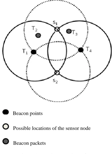
Suppose the list has four beacons {T1, T2, T3, T4} (as shown

in Fig 1). In the list two beacons which are the farthest from each other are chosen (T1, T4). These points are called as

Beacon points. These two points mark the end of the sensor node‟s communication range as the sensor node has not received a beacon farther from this point.

With those two points as centers and the communication range of a sensor node as radius, two circles are constructed (refer fig 1). Each circle represents the communication range of the mobile anchor which has sent the beacon, and so the sensor node has to fall inside the circle. Since the sensor node has received packets from both the anchors, the node falls inside both the circles. So the circles will intersect each other.

The intersection points of both the circles are determined (S1,

S2).The intersection points are the possible locations of the

sensor node. The reason is as follows. The two farthest points (Beacon Points) are the end points of a sensor node‟s communication range. So in the circle with the mobile anchor‟s position as the centre and the communication range of a node as the radius, the sensor node will be in the circumference of the circle.

Since it is the same with the other mobile anchor position, the sensor node lies on the circumference of the other circle also. So the sensor node lies on the circumference of both the circles. The points satisfying the above condition are the two intersection points. Hence at the end of phase I the location of the sensor node has been approximated to two locations.

3.2

Phase II

The second phase begins with two possible locations of the sensor node. The approach is based on the assumption that each sensor node measures its distance to mobile anchor when it sends a beacon using some technique like RSSI or TDOA. The accuracy improves when the number of measured distance is equal to or greater than three.

Beacon points

Possible locations of the sensor node

Beacon packets

Initialization

The solution space is constructed in and around the two possible locations determined at the end of phase I. Since the solution space is small the initial population size is less. Each individual in the population is a possible solution.

Genetic Encoding

Each individual is encoded as a real valued chromosome with two genes. First gene represents the location at x axis and second gene represents the location at y axis.

Selection

Selection is done on the population at hand to choose the fit parents. In this approach, Roulette wheel selection is used to determine the parents. Fitness function used is described as follows.

Fitness Function

Let m be the number of measured distances between the sensor node and the mobile anchor, when the mobile anchor is at various locations and di, i=1 to m are the actual distances

between the sensor node and mobile anchors when the anchors are at various locations (measured using any technique like RSSI). Finally (xi, yi), i=1 to m are the absolute

locations of the respective mobile anchors (obtained from the beacon packet).

Let (ai, bi), i=1 to n be estimated or possible locations of the

sensor node (initial population), where n is the size of initial population.

Equation (1) gives the distance between an individual in the population and a mobile anchor, i.e. estimated distance.



 



i i i

i

a

y

b

x







(1)

Based on this, fitness function is defined as, minimizing the difference between estimated distance and the actual distance between the sensor node and the mobile anchor. This is given by minimum of



 































m

i

i j i j

i n

j

x

a

y

b

d

1

2 2

2

1

(2)

Once the parents are chosen, arithmetic mutation and single point cross over are used for reproduction.

Arithmetic mutation

A small number of individuals are chosen from the selected population; for each individual, on any one of the axis ∆d is either added or subtracted. ∆d for that particular individual is calculated with respective (xi, yi) and (aj, bj).



 















_

_

_

_







d



x

a

y

b

d

(3)

where α ranges between 0.0 to 1.

After mutation, single point crossover is done on the parents to produce the children.

Selection, Reproduction is done iteratively till the termination condition is reached. When the difference between the distances has reached the minimum, the algorithm terminates.

4.

EXPERIMENTAL RESULTS

Table 1 Experimental setup

Number Of Sensor Nodes 100

Area of the Sensing Field 1000 X 1000 m2

Number of Mobile Anchors

3

Transmission range 250 m

Number of generations 10-60

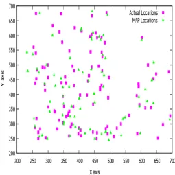
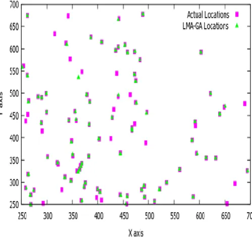
With the above experimental setup, the results were analyzed for both MAP and GA. Simulation of MAP and LMA-GA were done in NS-2. Graphs were plotted with Gnuplot. In fig 2 and fig 3, the actual locations of the sensor nodes and calculated locations are plotted. Fig 2 plots the locations obtained using MAP. Though the results show good localization, the accuracy is not as high as in LMA-GA. Fig 3 shows that using LMA-GA, the sensor nodes were localized with a very less difference from their actual location.

Figure 4 Difference in distance between Actual and Calculated locations in MAP and LMA-GA.

Fig 4 plots the difference in distance between the actual location and the calculated location. For each node (x axis), the impulse shows the difference in distance between MAP calculated location and actual location. For the same node, the point on the impulse marks the difference in distance between actual location and location estimated using LMA-GA. The graph shows a significant reduction in the localization error while using LMA-GA.

\

Fig 5 shows the Root Mean Square Error (RMSE) against number of iterations or generations in GA. MAP is independent of the number of generations. So the MAP plot does not vary with x-axis. It is observed that RMSE error of MAP varies, but always lies in the range as shown in fig 5.

But in the case of LMA-GA, as the number of iterations increases, RMSE error decreases gradually. The RMSE approaches zero when the number of iterations is 60. From fig 5 it is observed that RMSE of LMA-GA is very less compared to MAP.

5. CONCLUSION

From the experimental results it can be seen that LMA-GA gives very high localization accuracy as well as does not require extensive searching as in traditional Genetic algorithm. From the average error of MAP and LMA-GA methods obtained from the experimentation, it is observed that the percentage of localization error has decreased by 84%. LMA-GA also does not require expensive hardware as in range based methods and it does not require flooding of messages as in traditional range free algorithms. Thus it can be concluded that LMA-GA is a non-expensive and an efficient strategy that gives very high localization accuracy. Furthermore genetic algorithm can be combined with other evolutionary strategies like simulated annealing and hill climbing and the error of localization of the new hybrid genetic algorithm can be compared with the pure genetic algorithm (LMA-GA).

6. REFERENCES

[1] I.F.Akyildiz, W.Su, Y. Sankarasubramanium, E. Cayirci “Wireless Sensor Networks: a survey” IEEE communication. Mag., 2002, 40, (8), pp.102-114.

[2] Guoqiang Mao, Barıs¸ Fidan , Brian D.O. Anderson “Wireless Sensor Networks Localization Techniques “, Science Direct, Computer Networks 51, 2007,pp. 2599-2533.

[3] Guibin Zhu,Qiuhua Li, Peng Quan; Jiuzhi Ye “A GPS- free localization scheme for wireless sensor networks “, 12th IEEE International Conference on Communication Technology (ICCT 2010), Nov 2010, pp. 401-404, doi: 10.1109/ICCT.2010.5688823.

[4] Chaczko Zenon, Klempous Ryszard, Nikodem Jan, Nikodem Michal “Methods of Sensors Localization in Wireless Sensor Networks”, 14th Annual International

Figure 5. Comparison of Root Mean Square Error of

K MAP and LMA-GA

Conference and Workshops on Engineering on Computer based Systems (ECBS 2007), Mar 2007, pp. 145-152,doi: 10.1109/ECBS.2007.48.

[5] Yanping Zhu, Daqing Huang, Aimin Jiang “Network Localization using angle of arrival”, IEEE International Conference on Electro / Information Technology (EIT 2008), May 2008, pp. 205-210, doi: 10.1109/EIT.2008.4554297.

[6] Guowei Shen, Zetik R, Honghui Yan, Hirsch O., Thoma, R.S. “Time of Arrival Estimation for range-based localization in UWB sensor networks”,IEEE International Conference on Ultra-Wideband (ICUWB 2010), Sept 2010, Vol. 2, pp. 1-4, doi: 10.1109/ICUWB.2010.5614041.

[7] Pengfei Peng, Hao Luo, Zhong Liu, Xiongwei Ren “ A cooperative target location algorithm based on time difference of arrival in wireless sensor networks”, International Conference on Mechatronics and Automation (ICMA 2009), Aug 2009, pp. 696-701,doi: 10.1109/ICMA.2009.524601.

[8] Hoang Q.T., Le T.N., Yoan Shin “An RSS comparison based localization in wireless sensor networks”, 8th workshop on Positioning Navigation and communication (WPNC 2011), Apr 2011, pp. 116-121, doi: 10.1109/WPNC.2011.5961026.

[9] Zhang Zhao-yang, Gou Xu, Li Ya-peng, Shan-shan Huang “DV Hop Based Self-Adaptive Positioning in Wireless Sensor Networks”, 5th

International Conference On Wireless Communications, Networking and Mobile Computing (WiCom 2009), Sept 2009, pp. 1-4, doi: 10.1109/WICOM.2009.5301412.

[10]Binwei Deng, Guangming Huang, Lei Zhang, Hao Liu “Improved Centroid Localization Algorithms in WSNs”, 3rd _{International Conference on Intelligent System and}

Knowledge Engineering (ISKE 2008), Nov 2008, Vol. 1, pp. 1260-1264, doi: 10.1109/ISKE.2008.4731124.

[11]Patro, R.K. “Localization in wireless sensor network with mobile beacons”, 23rd _{IEEE convention of Electrical}

and Electronics Engineers Israel, Sept 2004, pp. 22-24, doi: 10.1109/EEEI.2004.136107.

[12]Kuo-Feng Ssu, Ou, C.-H., Jiau, H.C.: „Localization with mobile anchor points in wireless sensor networks‟, IEEE Trans. Veh. Technol., Vol. 54, (3), May 2005, pp. 1187– 1197, doi: 10.1109/TVT.2005.844642.

[13]Baoli Zhang, Fengqi Yu, Zusheng zhang “An Improved Localization Algorithm for Wireless Sensor Network Using a Mobile Anchor Node”, 2009 Asia-Pacific Conference on Information Processing.

[14]W-H Liao, Y.C.Lee, S.P. Kedia “Mobile anchor positioning of wireless sensor networks”, IET communications, 2011, Vol. 5, Issue 7, pp.914-921.

[15]Wenwen Li, Wuneng Zhou, “Genetic Algorithm- Base Localization Algorithm for Wireless Sensor Networks”, Seventh International Conference On Natural Computation (ICNC 11), July 2011, pp. 2096-2099, doi:10.1109/ICNC.2011.6022395.

7. AUTHORS PROFILE

S.Sivakumar was born in Tamilnadu, India in 1977. He

received his Bachelors degree B.E in Electronics and Communication from Bharathiyar University, Coimbatore in 1999. He completed his Masters degree M.E in Communication Systems from Anna University, Chennai in 2006. He is currently working as an Assistant Professor (Sr.Gr) in the Department of Information Technology at PSG College of Technology, Coimbatore, India. His research interests include Wireless Sensor Networks, Digital Signal Processing, Information coding Techniques and Networking.

Dr.R. Venkatesan was born in Tamilnadu, India, in 1958. He

received his B.E (Hons) degree from Madras University in 1980. He completed his Masters degree in Industrial Engineering from Madras University in 1982. He obtained his second Masters degree MS in Computer and Information Science from University of Michigan, USA in 1999. He was awarded with PhD from Anna University, Chennai in 2007. He is currently Professor and Head in the Department of Computer Science and Engineering at PSG College of Technology, Coimbatore, India. His research interests are in Simulation and Modeling, Software Engineering, Algorithm Design, Software Process Management.

M. Karthiga was born in Tamilnadu, India in 1988. She

received her Bachelors degree (B.Tech) in Information Technology from Amrita Viswa Vidya Peetham, Coimbatore in 2010. She is currently pursuing her Masters degree (M.E) in Computer Science and Engineering in PSG College of Technology, Coimbatore. Her research interest includes Wireless Sensor Networks, Operating Systems, Networks and

Evolutionary Computing