A Novel Stastical Particle Filtering Approach for Non Linear and Non Gaussian System Identification

(1)

A Novel Stastical Particle Filtering Approach for

Non-Linear and Non-Gaussian System Identification

Dhiraj K.Jha*

Dept. Of Electronics and Tele-

Communication Jadavpur University

Kolkata-32

Avinash Kumar

Kolkata-32

Prabhat Panda

Kolkata-32

Abhijit Verma

Kolkata-32

* Corresponding Author

ABSTRACT

Increasingly, for many application areas, it is becoming important to include elements of nonlinearity and non-Gaussianity in order to model accurately the underlying dynamics of a physical system. The problem of identifying nonlinear system models arise in various applications in control and signal processing. In this context, one of the most successful and popular stastical identification approaches is Particle Filtering, otherwise known as Sequential Monte Carlo (SMC) methods. As compared to Extended Kalman Filter and Gaussian Sum Filter, this approach is computationally reliable for identification of highly nonlinear systems in terms of accuracy, and, at the same time chance of failure in difficult circumstances decreases. The numerical integration techniques, on the other hand, are only feasible in low-dimensional state-spaces. In this paper the particle filtering approach has been attempted for non-linear system identification. The particles and their associated importance weights in particle filtering approach evolve randomly in time according to a simulation-based rule. This is equivalent to a dynamic grid approximation of the target distributions, where the regions of higher probability are allocated proportionally more grid positions. Using these particles Monte Carlo estimates of the quantities of interest may be obtained, with the accuracy of these estimates being independent of the dimension of the state space. The envisioned method is easier to implement than classical numerical methods and allows complex nonlinear and non-Gaussian estimation problems to be solved efficiently in an online manner. The experimental results on comparison with Kalman filtering show the efficacy of the proposed method through illustrative examples.

Index Terms

: Non-linear System, Kalman Filter, Bayesian Filter, Sequential Estimation, Particle Filter

1. INTRODUCTION

Problems in Engineering require estimation of the state of a system that changes over time using a sequence of noisy

measurements made on the system. The state-space approach to time-series modeling focuses attention on the state vector of a system. The state vector contains all relevant information required to describe the system under investigation. For example, in tracking problems, this information could be related to the kinematic characteristics of the target. The measurement vector represents (noisy) observations that are related to the state vector [1]. The measurement vector is generally (but not necessarily) of lower dimension than the state vector. The state space approach is convenient for handling multivariate data and nonlinear/non-Gaussian processes, and it provides a significant advantage over traditional time-series techniques for these problems [2]. In the Bayesian approach to dynamic state estimation, one attempts to construct the posterior probability density function (pdf) of the state based on all available information, including the set of received measurements. Since this pdf embodies all available statistical information, it may be said to be the complete solution to the estimation problem. In principle, an optimal (with respect to any criterion) estimate of the state may be obtained from the pdf. A measure of the accuracy of the estimate may also be obtained [3]. For many problems, an estimate is required every time that a measurement is received. Since the nineties, sequential Monte Carlo (SMC) approaches have become a powerful methodology to cope with non-linear and non-Gaussian problems [4].

(2)

Another approximation strategy is that of sequential Monte Carlo integration, also commonly known as particle methods.

The paper is organized as follows. Section II gives a brief description of theoretical foundations related to our approach. Section III describes the Bayesian Filtering. Section IV contains the prior approach to particle filtering approach as well as the illustrative model for Particle Filter. Section V shows the result along with the comparison result with Kalman Filtering approach. Section VI concludes the paper along with the directions for future research.

2. THEORETICAL FOUNDATIONS

General problem statement:

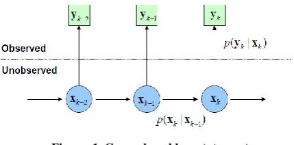
The particle filter is a sequential Monte Carlo algorithm, i.e. a sampling method for approximating a distribution that makes use of its temporal structure. A “particle representation “of distributions is used. In particular, we will be concerned with the distribution P(xt|z0:t) where xt is the unobserved state at time t, and z0: t is the sequence of observations from time 0 to time t.

[image:2.595.57.272.363.469.2]

Filtering is the problem of sequentially estimating the states (parameters or hidden variables) of a nonlinear system as a set of observations become available online.

Figure. 1. General problem statement

State space formulation of a system:

General discrete time nonlinear and non-Gaussian dynamic system is given by following equation:

(1)

Where

Xk = state,

Yk = noisy observation,

uk = known input

vk-1 = process noise,

nk = measurement noise

Assumptions for the state space formulation:

 State follow a first order markov process

 Observations independent given the states

3. NONLINEAR BAYESIAN FILTERING

Bayes rule is a very powerful tool for doing inference under conditions of uncertainty. For example, in robotics, perhaps the most frequent use of Bayes rule is to translate sensor readings into a map of the environment. Since the sensor readings are noisy, it is desirable to use Bayes rule to accumulate enough noisy measurements to localize obstacles in the world.

For a robot, it is undesirable to wait until it has gathered a bunch of sensor readings before it applies Bayes rule to give it a clue about the environment. Since robots are usually made to move, it is a good idea to use the information as it comes in to incrementally improve our understanding of the environment. To achieve this objective sequential estimation is generally used.

Sequential Estimation:

Sequential estimation is the process of incrementally

improving our understanding as data is gathered. The Bayes filter is a powerful tool for performing sequential estimation.

Suppose a physical process is described by a random variable, but there is no information is available about the behavior of the random variable. The first piece of information is the mean of this random variable. If pdf for this random variable is p(x), then mean can be expressed as

( )

xp x dx





_

(2)

If the pdf is not available, the estimate can be the mean by collecting samples of the process. Suppose n samples are represented by the set { x1,x2,…..,xn },Then sample mean is

given by 1

1

n i i

m

x

n





(3)

The problem with this is that all n samples should be collected before using the information. The trick is to come up with a difference equation that allows us to incrementally improve the estimate as data becomes available. Naturally, if only one sample is present, then the mean can be expressed as

m1 = x1.

mk can be written as any partial sum,

1

k k i i

m

x

k





(4)

mk can be further expressed as follows

1

k k i i

m

x

k





=

x

k

1

k +

k

1



  1 1 k i

x

i

=

x

k

1

k +

(3)

=

x

k

1

k +

k



1

(

1

1 

k







1

1 k i

x

i )

=

x

k

1

k +

m

k



1

k-1 (4)

This is the sequential estimate of the mean of a random variable.

Another form of sequential estimation is to sequentially estimate posterior distributions as actions are taken and as observations are made. If xK denote the state at time k, aK

denote the action taken at time k, and zK denote the

observation made at time k, then models can be used to show how actions produce consequences and how states are observed to improve estimates.

4. PARTICLE FILTER DESIGN

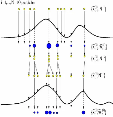
The sequential importance sampling (SIS) algorithm is a Monte Carlo (MC) method that forms the basis for most sequential MC filters developed over the past decades; see [4], [5]. This sequential MC (SMC) approach is known variously as bootstrap filtering [3], the condensation algorithm [6], particle filtering [7], interacting particle approximations [8], [9], and survival of the fittest [10]. It is a technique for implementing a recursive Bayesian filter by MC simulations. The key idea is to represent the required posterior density function by a set of random samples with associated weights and to compute estimates based on these samples and weights. As the number of samples becomes very large, this MC characterization becomes an equivalent representation to the usual functional description of the posterior pdf, and the SIS filter approaches the optimal Bayesian estimate.

Particle Filters originally developed for tracking application systems exclusively. It has the advantage over classical methods like spectral subtractions or Wiener filtering is that the particle filter allows the noise to be non-stationary. Particle filter is a technique for implementing recursive Bayesian filter by Monte Carlo sampling. The idea is to represent the posterior density by a set of random particles with associated weights. Compute estimates based on these samples and weights.

The steps for design of particle filter based model are as follows:

1. Representation of system.

2. Prediction of behavior of the system.

3. Measurement of prior sample of the signal.

4. Resampling of estimated particle.

[image:3.595.317.513.72.274.2]

The representations of the above steps are shown diagrammatically as follows:

Figure. 2. Particle Filter design

Choice of proposal distribution

:

Support of proposal distribution must include support of true posterior distribution, i.e. heavy tailed distributions are preferable. It must include most recent observations.

[image:3.595.319.513.421.545.2]

Generally most of the proposal distribution does not incorporate new observations. On the contrary, our approach incorporates new observations into the proposal by combining prior with the new observation using normalized Gaussian fusion strategy.

Figure. 3. New observation fusion with the prior

Nonlinear & non-Gaussian model

illustration:

Model – 1:

The unknown system is characterized as a basic non-linear model in this work. It is represented as the difference equation and is given as

X = 0.5*x+25*x/(1+x^2)+8*cos(1.2*(k-1))+ sqrt(q)*v(n)

Y = x^2 / 20 + sqrt(r) * v(n)

Where

x = 0.1; initial state

q = 1;

r = 1;

(4)

k varies from 1 to L

Model – 2:

Another model is developed and also tested for the accuracy result for such linearity change. By varying the non-linearity we can also examine the identification for both of the filter. The equation of the system is given by:

X=0.5*x+12*x/(1+x^2)+6*cos(1.2*(k-1))+ sqrt(q)*v(n)

Y = x^3 / 50 + sqrt(r)*v(n)

Where,

x = 0.1; initial state

q = 1;

r = 1;

v(n)=random noise

k varies from 1 to L

5. EXPERIMENTAL RESULTS

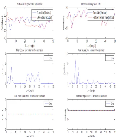
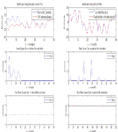
[image:4.595.336.531.82.302.2]

The result for the estimated model along with the Kalman Filter for different noise conditions are shown as follows:

[image:4.595.61.283.347.566.2]

Fig. 4. Result of Model 1. Kalman Filter (Left) and Particle Filter (Right) # instance 1

Fig. 5. Result of Model 1. Kalman Filter (Left) and Particle Filter (Right) for different values of random noise

# instance 2

Fig. 6. Result of Model 1. Kalman Filter (Left) and Particle Filter (Right) for different values of random noise

[image:4.595.337.533.403.635.2]

(5)

[image:5.595.63.280.76.298.2] [image:5.595.336.527.82.317.2]

[image:5.595.310.530.394.648.2]

TABLE 1. COMPARISION USING RMS ERROR

Instance Root mean square error_Kalman Filtering

Root mean square error_Particle Filtering

Model 1

#instance 1

16.4 2.1

Model 1

#instance 2

18.2 2.4

Model 1

#instance 3

11.5 1.9

Model 2

#instance 1

17.8 1.8

Model 2

#instance 2

10.1 2.0

Model 2

#instance 3

11.8 2.7

[image:5.595.76.279.398.625.2]

(6)

Hence, Identification using particle filter is advantageous than Kalman filter because tracking of nonlinear system by particle filter lies in nearly 95% confidence region.

Error for particle filter is less as compared to Kalman Filter.

Particle filters provide more accurate estimation about the unknown system provided simulated sample size is sufficiently large in comparison to extended or unscented Kalman filter.

Particle filtering is applicable to general nonlinear, non-Gaussian estimation problems where standard non-Gaussian approximations fail.

6. CONCLUSION AND FUTURE SCOPE

We proposed a novel stastical approach for nonlinear and nongaussian system identification using improved particle filtering with normalised Gaussian mixing of new observations with the priors. Experimental results show that our approach outperforms the Kalman filtering approach for system identification. In future, we will focus on implementation of particle filtering approach for nonlinear system identification under missing observations using evolutionary genetic filter. Another direction of future research is to implement particle filter for voice activity detection for real world applications.

7. REFERENCES

[1] M. Sanjeev Arulampalam, Simon Maskell, Neil Gordon, and Tim Clapp, “A Tutorial on Particle Filters for Online Nonlinear/Non-Gaussian Bayesian Tracking”, IEEE TRANSACTIONS ON SIGNAL PROCESSING, VOL. 50, NO. 2, pp- 174-188 , FEBRUARY 2002.

[2

]

R. H. Shumway and D. S. Stoffer, “An approach to time series smoothing and forecasting using the EM

algorithm,” J. Time Series Anal., vol. 3, no. 4, pp. 253– 264, 1982.

[3] N. Gordon, D. Salmond, and A. F. M. Smith, “Novel approach to nonlinear and non-Gaussian Bayesian state estimation,” Proc. Inst. Elect. Eng., F, vol. 140, pp. 107– 113, 1993.

[4] A. Doucet, J. F. G. de Freitas, and N. J. Gordon, “An introduction to sequential Monte Carlo methods,” in Sequential Monte Carlo Methods in Practice, A. Doucet, J. F. G. de Freitas, and N. J. Gordon, Eds. New York: Springer-Verlag, 2001.

[5] A. Doucet, S. Godsill, and C. Andrieu, “On sequential Monte Carlo sampling methods for Bayesian filtering,” Statist. Comput., vol. 10, no. 3, pp. 197–208.

[6] J. MacCormick and A. Blake, “A probabilistic exclusion principle for tracking multiple objects,” in Proc. Int. Conf. Comput. Vision, 1999, pp. 572–578.

[7] J. Carpenter, P. Clifford, and P. Fearnhead, “Improved particle filter for nonlinear problems,”Proc. Inst. Elect. Eng., Radar, Sonar, Navig., 1999.

[8] D. Crisan, P. Del Moral, and T. J. Lyons, “Non-linear filtering using branching and interacting particle systems,” Markov Processes Related Fields, vol. 5, no. 3, pp. 293–319, 1999.

[9] P. Del Moral, “Non-linear filtering: Interacting particle solution,” Markov Processes Related Fields, vol. 2, no. 4, pp. 555–580.