Classification of Cardiotocogram Data using Neural
Network based Machine Learning Technique
Sundar.C
Christian College of Engineering Technology,
Oddanchatram – 624619
M.Chitradevi
PRIST University Trichy Campus – Tamilnadu
Tiruchirappalli – 620 009
Dr.G.Geetharamani
Anna University of Technology
Tiruchirappalli - 620024
ABSTRACT
Cardiotocography (CTG) is a simultaneous recording of fetal heart rate (FHR) and uterine contractions (UC). It is one of the most common diagnostic techniques to evaluate maternal and fetal well-being during pregnancy and before delivery. By observing the Cardiotocography trace patterns doctors can understand the state of the fetus. There are several signal processing and computer programming based techniques for interpreting a typical Cardiotocography data. Even few decades after the introduction of cardiotocography into clinical practice, the predictive capacity of the these methods remains controversial and still inaccurate. In this paper, we implement a model based CTG data classification system using a supervised artificial neural network(ANN) which can classify the CTG data based on its training data. According to the arrived results, the performance of the supervised machine learning based classification approach provided significant performance. We used Precision, Recall, F-Score and Rand Index as the metric to evaluate the performance. It was found that, the ANN based classifier was capable of identifying Normal, Suspicious and Pathologic condition, from the nature of CTG data with very good accuracy.
Keywords
Multidimensional Data Classification, Medical Data Classification, Cardiotocography, CTG, fetal heart rate, FHR. uterine contractions, UC, ANN
.
1. INTRODUCTION
Data Mining (DM) and the technology of Knowledge Discovery from Data (KDD) has brought many new developments, methods, and technologies in the recent decade. Also the improvement of integration of techniques and the application of data mining techniques had contributed in handling of new kinds of data types and applications. However, the field of data mining and its application in medical domain is still young enough so that the possibilities of the application are still limitless [20].
One of the major challenges in medical domain is the extraction of comprehensible knowledge from medical diagnosis data such as CTG data. In this information era, the use of machine learning tools in medical diagnosis is increasing gradually. This is mainly because the effectiveness of classification and recognition systems has improved in a great deal to help medical experts in diagnosing diseases[21].
1.1 Cardiotocography (CTG)
Cardiotocography (CTG) is a technical means of recording the fetal heart rate (FHR) and the uterine contractions (UC) during pregnancy, typically in the third trimester to evaluate maternal and fetal well-being. FHR patterns are observed manually by obstetricians during the process of CTG analysis.
In the recent past fetal heart rate baseline and its frequency analysis has been taken in to research on many aspects [2],[6].
Fetal heart rate (FHR) monitoring is mainly used to find out the amount of oxygen a fetus is acquiring during the time of labor [7]. Even then death and long term disablement occurs due to hypoxia during delivery. More than 50% of these deaths were caused by not recognizing the abnormal FHR pattern, even after recognizing not communicating the same without knowing the seriousness and the delay in taking appropriate action [7]. The currently proposed computation and datamining techniques for FHR can be used for analyzing and classifying the CTG data to avoid human mistakes and helps the doctors to take a decision.
2. PROBLEM DEFINITION
Cardiotocography (CTG), consisting of fetal heart rate (FHR) and tocographic (TOCO) measurements, is used to evaluate fetal well-being during the delivery. Since 1970 many researchers have employed different methods to help the doctors to interpret the CTG trace pattern from the field of signal processing and computer programming [2]. They have supported doctors with interpretations in order to reach a satisfactory level of reliability so as to act as a decision support system in obstetrics. Up to now, none of them has been adopted worldwide for everyday practice (Van Geijnt, 1996). There is currently no consensus on the best methodology for baseline estimation in computer analysis of cardiotocographs [2]. More than 30 years after the introduction of antepartum cardiotocography into clinical practice, the predictive capacity of the method remains controversial. In a review of lot of articles published on this subject, it was found that its reported sensitivity varies between 2 and 100%, and its specificity between 37 and 100% [5]. So, in this work, we are going to evaluate some of the statistical, machine learning and datamining techniques for the classification of CTG data.
As means of data collection have become more capable, the need for non-linear modeling techniques has become more and more apparent. Traditional statistical methods rely on an assumption of linearity. However, since most of the data collected concerns, or is the result of, human behavior, and humans rarely behave linearly, methods that assume linear separability are ultimately doomed to failure. Furthermore, data collection streams are broadening. The number of variables of concern to modelers has increased by at least an order of magnitude. Traditional methods simply were not designed to work with one hundred or more variables.
In answer to this, the last decade has seen the emergence of neural networks as a means of non-linear modeling. These devices resulted from the efforts of a number of cognitive scientists to mimic learning and memory in the human brain. The back-propagation neural network in particular has proven successful in creating useful models from large masses of complex data. The algorithm has been successfully applied in a variety of settings including direct marketing, intelligence and process control. Because of its pattern recognition nature it has proven robust with respect to missing data and other data irregularities.
2.1
The
Medical
Background
Of
Cardiotocography (CTG)
Cardiotocography is a medical test conducted during pregnancy that records fetal heart rate(FHR) and uterine contractions. The tests may be conducted by either internal or external methods. In internal testing, a catheter is placed in the uterus after a specific amount of dilation has taken place. With external tests, a pair of sensory nodes is affixed to the mother's stomach. The CTG trace generally shows two lines. The upper line is a record of the fetal heart rate in beats per minute. The lower line is a recording of uterine contractions from the TOCO [4].
2.1 Baseline Heart Rate
The baseline heart rate helps to evaluate the healthy functioning of the cardiovascular system. The baseline fetal heart rate is determined by approximating the mean FHR rounded to increments of 5 beats per minute (bpm) during a 10-minute window, excluding accelerations and decelerations and periods of marked FHR variability (greater than 25 bpm. Abnormal baseline is termed bradycardia and tachycardia.
The fluctuations are visually quantitated as the amplitude of the peak- to-trough in bpm. Using this definition, the baseline FHR variability is categorized by the quantitated amplitude as:
Absent- undetectable
Minimal- greater than undetectable, but less than or equal to 5 bpm
Moderate- 6 bpm - 25 bpm
Marked- greater than 25 bpm
Bradycardia: It is the resting heart rate of under 60 beats
per minute, though it is seldom symptomatic until the rate drops below 50 beats/min. It may cause cardiac arrest in some patientsTachycardia: It typically refers to a heart rate that
exceeds the normal range for a resting heart rate (heart rate in an inactive or sleeping individual). It can be dangerous depending on the speed and type of rhythm.Type 1 (early)
This occurs during the peak of the uterine contraction. It will be uniform, repetitive, periodic slowing of FHR with onset early in the contraction and return to baseline at the end of the contraction. The reasons behind this may be fetal head compression, cord compression or early hypoxia. This occurs in first and second stage labor with decent of the head [4]. This is synchronous with uterine contraction
Type 2 (late)
This occurs after the peak of the uterine contraction. It will also be uniform, repetitive, slowing of FHR with onset mid to end of the contraction and nadir more than 20 seconds after the peak of the contraction and ending after the contraction. If the lag time is high seriousness is also high. This is also synchronous with uterine contraction. Mx: a fetal pH measurement is mandatory [4].
Type 3 (variable)
This is variable, repetitive, periodic slowing of FHR with rapid onset and recovery. Variable and isolated time relationships with contraction cycles may occur. In some cases, they resemble other types of deceleration patterns in timing and shape. If they occur consistently, there is a chance of fetal hypoxia. This is unrelated to uterine contractions. Mx: check fetal pH if the pattern persists after turning the patient on her side (or if other adverse features are present) [4].
3.
CLASSIFICATION
USING
ARTIFICIAL NEURAL NETWORK
3.1 ANN Based Classification
Here in this classification, we use supervised learning by using a set of training data which is accompanied by class labels. When a new data arrive, then classification of that data will be done based on the training set by generating descriptions of the classes. In addition to training set we also have a test data set that is used to determine the effectiveness of a classification. In general, commonly used and popular neural networks can be trained to recognize the data directly, whereas in simple networks there is a chance of the system being complex and training may be difficult. The time taken and the accuracy of classification depend on the dimension of the input given and also on the dimension in the training data. For input data with high dimension, the process will take a longer time.
3.2 Structuring the Network
The number of layers and the number of processing elements per layer are important decisions. These parameters to a feed forward, back-propagation topology are also the most ethereal - they are the "art" of the network designer. There is no quantifiable, best answer to the layout of the network for any particular application. There are only general rules picked up over time and followed by most researchers and engineers applying this architecture to their problems.
Rule One: As the complexity in the relationship between
the input data and the desired output increases, the number of the processing elements in the hidden layer should also increase.required. If the process is not separable into stages, then additional layers may simply enable memorization of the training set, and not a true general solution effective with other data.
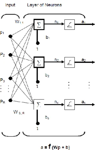
Fig 1: Feed forward Network
Rule Three: The amount of training data available sets an
upper bound for the number of processing elements in the hidden layer(s). To calculate this upper bound, use the number of cases in the training data set and divide that number by the sum of the number of nodes in the input and output layers in the network. Then divide that result again by a scaling factor between five and ten. Larger scaling factors are used for relatively less noisy data. If you use too many artificial neurons the training set will be memorized. If that happens, generalization of the data will not occur, making the network useless on new data sets.A single-layer network of S logsig neurons having R inputs is shown below in full detail on the left and with a layer diagram on the right [16].
Feed forward networks often have one or more hidden layers of sigmoid neurons followed by an output layer of linear neurons [11], Multiple layers of neurons with nonlinear
transfer functions allow the network to learn nonlinear and linear relationships between input and output vectors. The linear output layer lets the network produce values outside the range -1 to +1. On the other hand, if you want to constrain the outputs of a network (such as between 0 and 1), then the output layer should use a sigmoid transfer function.
3.3 The ANN based CTG Data
Classification System
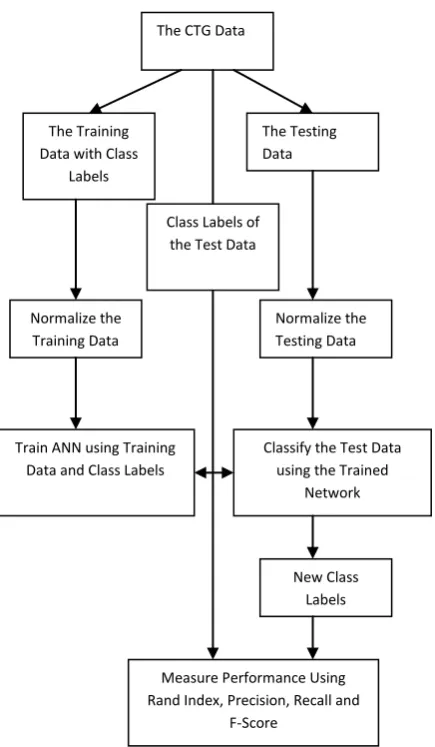
The Fig. 2 shows the ANN based CTG data Classification system.
The Metrics Used for the Evaluation
Precision, recall and F-Score are computed for every (class, cluster) pair. But Rand index is a metric which will consider all the classes and the clusters as the whole.
Rand Index
The Rand index or Rand measure is a commonly used technique for measure of such similarity between two data clusters.
Given a set of n objects S = {O1, ..., On} and two data clusters of S which we want to compare: X = {x1, ..., xR} and Y = {y1, ..., yS} where the different partitions of X and Y are disjoint and their union is equal to S; we can compute the following values:
a is the number of elements in S that are in the same partition in X and in the same partition in Y,
b is the number of elements in S that are not in the same partition in X and not in the same partition in Y,
c is the number of elements in S that are in the same partition in X and not in the same partition in Y,
d is the number of elements in S that are not in the same partition in X but are in the same partition in Y.
Fig 2: The ANN based CTG Data Classifier
d
c
b
a
d
a
RI
The Rand index has a value between 0 and 1 with 0 indicating that the two set of data clusters do not agree on any pair of points and 1 indicating that the two data clusters are exactly similar.
Precision
Precision is calculated as the fraction of correct objects among those that the algorithm believes belonging to the relevant class. It can be loosely equated to accuracy and it will roughly answers the question: “How many of the points in this cluster belong there/ correctly classified?”
The Precision is calculated as : P(Lr, Si) = nri/ni
for
class Lr of size nr
cluster Si if size ni
nri data points in Si from class Lr
Recall
Recall roughly answers the question: "Did all of the documents that belong in this cluster make it in?". In other words, recall is the fraction of actual objects that were identified.
The recall is calculated as : R(Lr, Si) = nri/nr
F-Score
F-Score is the harmonic mean of Precision and Recall and will tries to give a good combination of the two. It is calculated with the equation:
)
,
(
)
,
(
)
,
(
)
,
(
2
)
,
(
i r i r i r i r i rS
L
P
S
L
R
S
L
P
S
L
R
S
L
F
4.
RESULTS
AND
DISCUSSION
4.1 Data Set Information
For evaluating the algorithms under consideration, we used cardiotocograms data from UCI Machine Learning Repository.
This data set contains 2126 fetal cardiotocograms belonging to different classes. The data contains 21 attributes and two class labels. The CTGs were classified by three expert obstetricians and a consensus classification label assigned to each of them. Classification was both with respect to a morphologic pattern (A, B, C. ...) and to a fetal state (N, S, P). Therefore the dataset can be used either for 10-class or 3-class experiments. Here we use this data set for these evaluations.
Attribute Information
1) LB - FHR baseline (beats per minute)
2) AC - # of accelerations per second
3) FM - # of fetal movements per second
4) UC - # of uterine contractions per second
5) DL - # of light decelerations per second
6) DS - # of severe decelerations per second
7) DP - # of prolongued decelerations per second
8) ASTV - percentage of time with abnormal short term variability
9) MSTV - mean value of short term variability
10) ALTV - percentage of time with abnormal long term variability
11) MLTV - mean value of long term variability
12) Width - width of FHR histogram
13) Min - minimum of FHR histogram
14) Max - Maximum of FHR histogram
15) Nmax - # of histogram peaks
16) Nzeros - # of histogram zeros
17) Mode - histogram mode
18) Mean - histogram mean
19) Median - histogram median
20) Variance - histogram variance
21) Tendency - histogram tendency
The CTG Data
The Training Data with Class
Labels The Testing Data Normalize the Training Data Normalize the Testing Data
Train ANN using Training Data and Class Labels
Classify the Test Data using the Trained
Network
New Class Labels Class Labels of
the Test Data
Measure Performance Using Rand Index, Precision, Recall and
22) CLASS - FHR pattern class code (1 to 10)
23) NSP - fetal state class code (Normal=1; Suspect=2; Pathologic=3)
Class Information
We used the data for a three class classification problem. The descriptions for the three classes are
Normal
A CTG where all four features fall into the reassuring category
Suspicious
A CTG whose features fall into one of the non-reassuring categories and the non-reassuring category and the remainder of features are reassuring
Pathological
A CTG whose features fall into two or more of the Non-reassuring the Non-reassuring category or two or more abnormal categories.
4.2 The Visualization of Data Space
[image:5.595.319.512.76.381.2]The following image shows the projection of this 21 attribute (dimension) data in to a virtual three dimensional data space. We used three principal components of the data for this projection. In this plot, the normal CTG data points are shown in black dots, the suspicious data points are shown as blue dots, and the Pathologic data points are shown as red ‘x’ mark. This figure roughly shows the distribution of the data in the virtual space.
Fig 1 : The 3D projection of CTG data
The Numerical Results
[image:5.595.316.541.407.520.2]The following tables show the average performance of the three different methods. Here we tabulate the average results of ten trials. (The detailed results of all the trials can be found in the tables presented in annexure section)
[image:5.595.53.260.409.608.2]Table 1.The Performance in terms of Rand Index and CPU time
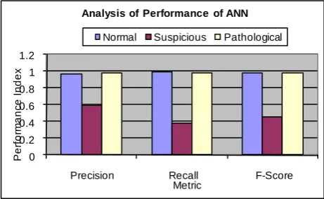
Table 2. The Average Performance of ANN Based Classifier
Metric Normal Suspicious Pathological
Precision 0.9663 0.5897 0.9706
Recall 0.991 0.3688 0.9745
F-Score 0.9784 0.4514 0.9724
The Analysis of Results
The performance of the algorithms in terms of Rand Index was good and always greater than 0.9. The proposed model consumed around 2.5 seconds for training and testing. 2.5 seconds is not a big figure to consider and will not be a obstacle in practical use of the method in real world application.
0 0.2 0.4 0.6 0.8 1 1.2
Precision Recall F-Score
P
e
rf
o
rm
a
n
ce
I
n
d
e
x
Metric
Analysis of Performance of ANN
Normal Suspicious Pathological
Fig 4. Performance of ANN
SlNo RI Time
01 0.9146 3.6719
02 0.9428 2.4844
03 0.9317 2.3750
04 0.9266 2.5469
05 0.9396 2.3750
06 0.9481 2.4688
07 0.9395 2.3750
08 0.9325 2.4688
09 0.9348 2.4531
10 0.9178 2.6719
[image:5.595.319.550.592.734.2]The above chart (Fig. 4) obviously shows the good performance of ANN based classifier. It gives good precision, recall and f-score for normal as well as pathological
records. But giving poor performance in the case of suspicious records.
Arrived results obviously show that supervised machine learning based methods can be used for the classification of CTG data. We realize that there are some training glitches in the case of suspicious records which caused some unexpected poor results while classifying the CTG data class “suspicious”.
5. CONCLUSION
The performance neural network based classification model has been analyzed with CTG dataset.. According to the arrived results, the performance of the supervised machine learning based classification approach provided significant performance. It was found that, the ANN based classifier was capable of identifying Normal, Suspicious and Pathologic condition, from the nature of CTG data with very good accuracy. ANN based classifier provided excellent performance in terms of Rand Index, Precision, Recall and F-Score. It was capable of identifying Normal and Pathologic condition with almost equal accuracy. But if we carefully see the comparative chart of ANN (the last figure), we can tell that, it’s performance to identify the Suspicious CTG pattern
is little bit poor than the other two classes. So future works my address the way to improve the system to recognize the Suspicious CTG patterns with the same accuracy.
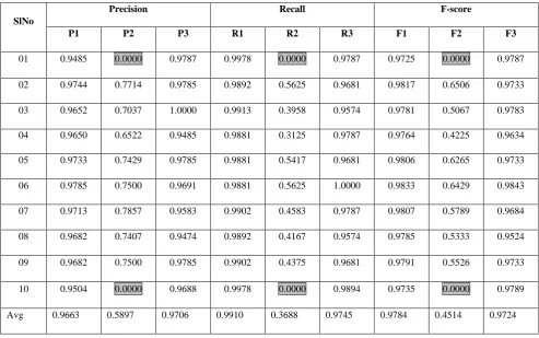
Even though the ANN based classifier provided excellent average performance, if we carefully watch the results of ten trials with ANN (the last table in annexure), we may find another weakness of this system. If we see some cells of the columns P2, R2 and F2 there are some bad results (highlighted in gray colour) during some trials. It means, in that trial, the system was absolutely incapable of identifying a single suspicious record. It means, even though we train the system with all the classes of samples, there is a chance by which the trained system may be incapable of identifying suspicious record. That is why we are getting comparatively poor average performance while classifying suspicious records. It is a major weakness of the system which should be overcome in future design. One may address the way to improve the system for getting proper training with different classes of CTG patterns. Future works may address hybrid models using statistical and machine learning techniques for improved classification accuracy.
A
NNEXURE-
1
[image:6.595.48.542.405.714.2]In the following tables, P1 is the precision for normal record, P2 is the precision for suspicious record, P3 is the precision for pathological records. R1 is the recall for normal record, R2 is the recall for suspicious record, R3 is the recall for pathological records. F1 is the f-score for normal record, F2 is the f-score for suspicious records, F3 is the f-score for pathological records.
Table 3. Results with ANN (10 Trials)
SlNo
Precision Recall F-score
P1 P2 P3 R1 R2 R3 F1 F2 F3
01 0.9485 0.0000 0.9787 0.9978 0.0000 0.9787 0.9725 0.0000 0.9787
02 0.9744 0.7714 0.9785 0.9892 0.5625 0.9681 0.9817 0.6506 0.9733
03 0.9652 0.7037 1.0000 0.9913 0.3958 0.9574 0.9781 0.5067 0.9783
04 0.9650 0.6522 0.9485 0.9881 0.3125 0.9787 0.9764 0.4225 0.9634
05 0.9733 0.7429 0.9785 0.9881 0.5417 0.9681 0.9806 0.6265 0.9733
06 0.9785 0.7500 0.9691 0.9881 0.5625 1.0000 0.9833 0.6429 0.9843
07 0.9713 0.7857 0.9583 0.9902 0.4583 0.9787 0.9807 0.5789 0.9684
08 0.9682 0.7407 0.9474 0.9892 0.4167 0.9574 0.9785 0.5333 0.9524
09 0.9682 0.7500 0.9785 0.9902 0.4375 0.9681 0.9791 0.5526 0.9733
10 0.9504 0.0000 0.9688 0.9978 0.0000 0.9894 0.9735 0.0000 0.9789
6. REFERENCES
[1] Xiaojun Chen, Yunming Ye, Xiaofei Xu, Joshua Zhexue Huang , “A feature group weighting method for subspace clustering of high-dimensional data”, Pattern Recognition 45 (2012) 434-446, Elsevier
[2] Shahad Nidhal, M. A. Mohd. Ali1 and Hind Najah, “A novel cardiotocography fetal heart rate baseline estimation algorithm”, Scientific Research and Essays Vol. 5(24), pp. 4002-4010, 18 December, 2010
[3] ANA. KLIMEŠOVÁ, EVA OCELÍKOVÁ,
Multidimensional Data Classification, Proceedings of the 10th WSEAS International Conference on AUTOMATION & INFORMATION, ISSN: 1790-5117, ISBN: 978-960-474-064-2
[4] Stirrat, Mills and Draycott, "Notes on Obstetrics and Gynaecology for the MRCOG, 5th Edition", 04 Aug 2003, ISBN: 9780443072239
[5] Diogo Ayres-de-Camposa, Cristina Costa-Santosb, Joa˜o Bernardesa, "Prediction of neonatal state by computer analysis of fetal heart rate tracings: the antepartum arm of the SisPorto1 multicentre validation study”, European Journal of Obstetrics & Gynecology and Reproductive Biology 118 (2005) 52-60.
[6] http://www.academicjournals.org/SRE, ISSN 1992 – 2248 © 2010 Academic Journals.
[7] Antonia Costa, MD; Diogo Ayres-de-Campos, PhD; Fernada Costa, MD; Cristina Santos, MS; Joao Bernardes, PhD, “Prediction of neonatal academia by Computer analysis of fetal heart rate and ST event sibnals” 2009 AJOG – American Journal of Obstetrics and Gynecology.
[8] Ben Kao, Sau Dan Lee, Foris K.F.Lee, David W. Cheung, Wai-Shing Ho,” Clustering Uncertain Data using Voronoi Diagrams and R-Tree Index” IEEE Transactions on Knowledge and Data Engineering, Vol. 22(9), pp. 1219 – 1233, sep 2010
[9] E. Ocelikova, D. Klimesova, “ Bays Classifier in multidimensional data classification “ 15th
Int. Conference Process Control 2005, pp. 188-1 – 188-5. Strbske Pleso, Slovakia.
[10] E. Ocelikovć, J Krištof, “Classification of multispectral
data” Zbornik radova, Volume 25, Number 1(2001).
[11] http://www-h.eng.cam.ac.uk/help/tpl/programs/ matlab.html.
[12] S.Anto, Dr. S.Chandramathi, “Supervised Machine Learning Approaches for Medical Data Set Classification – A Review” IJCST Nol. No.2, Issue 4, pp. 234 – 240, Oct – Dec 2011, ISSN : 2229-4333.
[13] Frank, A. Asuncion, UCI Machine Learning Repository {http://archive.ics.uci.edu/ml}, 2010.
[14] Zhaohong Deng , Kup-Sze Choi , Fu-Lai Chung , Shitong Wang, Enhanced soft subspace clustering integrating within-cluster and between-cluster information, Pattern Recognition, v.43 n.3, p.767-781, March, 2010 [doi>10.1016/j.patcog.2009.09.010]
[15] Hans-Peter Kriegel , Peer Kröger , Arthur Zimek, Clustering high-dimensional data: A survey on subspace clustering, pattern-based clustering, and correlation clustering, ACM Transactions on Knowledge Discovery from Data (TKDD), v.3 n.1, p.1-58, March 2009 [doi>10.1145/1497577.1497578]
[16] http://www.mathworks.in/help/toolbox/nnet/ug/bss33y1-1.html.
[17] S.Angle Latha Mary, K.R.Shankar Kumar,” Evaluation of Clustering Algorithm with Cluster Validation Metrics” European Journal of Scientific Research ISSN 1450-216X Vol.69 No.1 (2012), pp.61-72
[18] https://sites.google.com/site/dataclusteringalgorithms/fuz zy-c-means-clustering-algorithm.
[19] http://home.dei.polimi.it/matteucc/Clustering/tutorial_ht ml/cmeans.html.
[20] YI PENG, GANG KOU“A descriptive framework for
the field of data mining and knowledge discovery” International Journal of Information Technology & Decision Making Vol. 7, No. 4 (2008) pp. 639–682.