Neural Internal Model Control for tracking Unknown
Nonaffine Nonlinear Discrete-time Systems under
External Disturbances
T. A. A. Alzohairy
Assistant Proffessor Community College in Arriyadh
King Saud University
ABSTRACT
Tracking of nonlinear dynamic plants under external disturbances is presently an active area of research. The main difficulty felt in the tracking of nonlinear dynamic plants under external disturbances is the computational complexity in control design. This paper presents a simple neural network internal model control (IMC) approach for off-line tracking of unknown nonaffine nonlinear discrete time systems subject to external disturbances. The proposed control scheme is based on the neural network plant model and the inverse model. These models are determined using input output data. The final neural network IMC approach, including network plant model and the inverse model, is work off-line for tracking nonaffine nonlinear discrete time systems subject to external disturbances. Simulation results have been presented toward the end of the paper to illustrate the effectiveness of the proposed control strategy for tracking unknown nonaffine nonlinear discrete-time systems with and without external disturbances.
General Terms
Control systems, Neural networks, Nonlinear systems.
Keywords
Input-output approximation, Inverse model, Multilayer perceptron, Nonlinear Internal Model Control (IMC), Nonaffine nonlinear discrete-time system, Single input single output (SISO) systems.
1.
INTRODUCTION
Artificial neural networks (ANNs) have shown an excellent ability to model any nonlinear function to a desired degree of accuracy [8]. Because of this property, they are suitable for the identification and control of nonlinear plants [14]. From the different classes of networks, feedforward neural networks and particularly multi-layer perceptrons (MLPs) are the most frequently used for nonlinear control.
In recent years there has been a significant increase in the number of neural network based control techniques. One such method is the neural network internal model control (IMC) strategy. This strategy is one of the important techniques used for the control of unknown nonlinear discrete-time systems subject to uncertainainties (model mismatch and disturbances) because of its robustness against uncertainties [2],[4], [5], [9], [11] ,[21]. The IMC-based ANN strategy consists of training a network to learn the plant dynamics. Another neural network is trained to learn the inverse dynamics so that it can be used as a nonlinear controller.
In general the inversion of nonlinear models is not an easy task and analytical solutions may not exist, so solutions have to be found numerically. One important point is that the inversion of the plant model may lead to unstable controllers when the plant has unstable zeros. Fortunately, there are several strategies for obtaining the inverse model so that the nonlinear performance can be fully exploited in order to cope with a complex plant [3].
It is well known that nonaffine nonlinear plant models represent a much broader group of both real-world and academic systems. For an unknown nonaffine nonlinear discrete-time system, its output depends nonlinearly on its input. Therefore, it is no longer a simple task to determine the control input of such a nonaffine nonlinear system.
Most frequently used nonaffine nonlinear discrete-time systems are described by the nonlinear autoregressive moving average with eXogenous input (NARMAX) representation [1].
Recently, neural network control for unknown nonaffine nonlinear discrete-time systems has received considerable attention for its academic challenge and its practical interest. Adaptive neural network for such nonlinear systems based on online identification with backpropagation is given in [16]. The study of adaptive inverse control in which dynamic gradient methods were used to adjust the neural networks weights is given in [17]. Control of nonaffine nonlinear discrete-time systems using reinforcement learnining based linearly parameterized neural networks is given in [19].
All of the above mentioned results and others are limited to on-line control. In this paper the plant NARMAX representation and IMC based on artificial neural networks are used to produce an efficient off-line control scheme for tracking unknown nonaffine nonlinear discrete-time systems under external disturbances. As we will see in the simulation results, the neural network IMC strategy shows satisfactory performance when it is used to control unknown nonaffine nonlinear discrete-time systems with and without disturbances.
diagram of the internal model control (IMC) structure with details of the implementation of model and inverse is given in section 6. Section 7 presents the simulation results for tracking SISO nonaffine nonlinear discrete-time systems with or without disturbances. A comparison study when control SISO nonaffine nonlinear discrete-time systems done with and without disturbances is shown in section 8. Finally, some conclusions are remarked in Section 9.
2.
STATEMENT OF THE PROBLEM
Consider the following SISO nonaffine nonlinear discrete-time system [20]:
)] k ( X [ h ) 1 k ( y
] u(k) ), k ( X [ s ) 1 k ( x
) k ( x ) 1 k ( x
) k ( x ) 1 k ( x
n
3 2
2 1
(1)
where X(k)
x1(k),x2(k),,xn(k)
TRn is the internal state of the system, u(k)Ris the input to the system,R ) k (
y is the measured output, and s(.) and h(.) are unknown smooth nonlinear functions.
The control objective is to design a control input u(k), such that the system output y(k) subjected to disturbances d follows a known and bounded trajectory r(k)R.
3.
NONLINEAR IMC USING NEURAL
NETWORKS
For the control of nonlinear discrete-time systems subject to uncertainties (model mismatch and disturbances)nonlinear internal model control (IMC) using neural networks has received much attention [10], [12], [18]. Nonlinear IMC was proposed by [6], as shown in Fig. 1. The key characteristic of this type of control strategy is to have the inverse controller and the internal model. In Fig. 1, the model of the nonlinear plant is needed as the internal model. Using this internal model, the effect of uncertainties can be suppressed with the feedback signal generated. In nonlinear IMC, the nonlinear model and its inversion play a crucial role. Fig. 2 gives a basic neural network IMC structure [15], which is an extension of nonlinear IMC. For the control of unknown nonlinear discrete systems using the nonlinear IMC structure, neural network model is employed as the internal model and neural network inverse controller is used to replace the inverse controller, as shown in Fig. 2. The control structure given in Figs. 1 and 2 has been shown to have good robustness against uncertainties [10], [11], [12].
[image:2.595.320.543.74.186.2]Fig.1: Basic Structure of nonlinear IMC.
Fig. 2: Basic Structure of NN IMC.
4.
NN MODELING
The first step in performing control using IMC strategy is to find model of the plant. The model of the plant should capture the dynamics of the plant well enough so that a controller designed to control the plant model will also control the plant very well.
For convenience of analysis, the future output of the SISO nonaffine nonlinear discrete-time system (1) is determined by a number of past observations of the inputs and outputs. An equivalent input-output representation can be written as the nonlinear auto regressive moving average with exogenous inputs (NARMAX) system:
] 1) m -u(k , 1), -u(k u(k),
1), n -y(k , 1), -y(k ), k ( y [ f ) 1 k ( y
(2)
where n and m are the highest orders of the output and input, respectively, (.)f is the smooth nonlinear function.
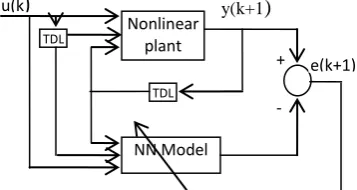
[image:2.595.340.519.597.692.2]The series-parallel identification model corresponding to a plant represented by (2) has the form shown in Fig. 3. TDL in Fig. 3 denotes a tapped delay line whose output vector has for its elements the delayed values of input signal. Hence the past values of the input and the output of the plant form the input vector to a neural network whose output yˆ(k1) corresponds to the estimate of the plant output at any instant of timek1. The series-parallel model enjoys several advantages: 1) since the plant is assumed to be BIBO stable, all the signals used in the identification procedure are bounded. 2) since no feedback loop exists in the model, static back propagation can be used to adjust parameters reducing the computational overhead substantially. 3) assume that the output error tends to small value asymptotically i.e., yˆ(k1)y(k1), the series-parallel model may be replaced by a series-parallel model without serious consequences. This has practical implications if the identification model is to be used off line.
Fig. 3: Architecture for finding neural network internal model of the nonaffine plant represented by a NARMAX model (2).
In this paper, a multilayer network with an input layer, an output layer with one neuron, and two hidden layers is used to model the nonaffine plant represented by a NARMAX model (2).
Robustness Filter
NN Inverse
Controller Nonlinear Plant
NN Model y(k)
e(k)
r(k) u(k)
+
-
+
-DisturbancesRobustness Filter
Inverse Controlle
r
Nonlinear Plant
Internal Model Internal
Model y(k)
e(k)
r(k) u(k)
+
-
+
-Disturbances Nonlinear plant
Nonlinear plant
NN Model
TDL TDL
) 1 k ( yˆ
e(k+1)
y(k+1
)
+
[image:2.595.56.281.615.723.2]The multilayer network performs the calculations such that the output of the jth neuron in 1st and the output of the rth neuron in 2nd hidden layers are expressed as
i 1 h j i 1 h ji 1 h jj f w X b
I (3)
j 2 h r j 2 h rj 2 h rr f w I b
Z (4)
Where X is the i ith network input, whji1 is the connection
weight from the ith input to the jth neuron in the 1st hidden layer, whrj2 is the connection weight from the jth neuron in the 1st hidden layer to the rth neuron in the 2nd hidden layer,
1 h j
b is the weight from the bias to the jth neuron in the 1st hidden layer, bhr2 is the weight from the bias to the rth
neuron in the second hidden layer, fjh1(.) and frh2(.) are
nonlinear sigmoid activation functions defined as
netinput e 1 1 ) netinput ( f
(5)
The network output is calculated by the following equation
r o r o r o b Z w f ) 1 k (yˆ (6)
where w is the weight connection of the neuron in the or
output layer to the rth neuron in the 2nd hidden layer, b is o the bias weight for the output neuron, and f is the o
transformation function between 2nd hidden layer and output layer and it is a linear function.
The popular backpropagation algorithm for training the multilayer network is gradient descent-based algorithm to minimize the following cost function
2 )) 1 k ( yˆ ) 1 k ( y ( 2 1
J (7)
A recursive algorithm, starting at the output nodes and working back to the first hidden layer is used to adjust weights, is given by
X ) k ( w ) 1 k ( w I ) k ( w ) 1 k ( w Z ) k ( w ) 1 k ( w i 1 h j 1 h ji 1 h ji j 2 h r 2 h rj 2 h rj r o o r o r (8)
where is the learning rate 01 and
r 2 h rj 2 h r j j 1 h j o r o r r 2 h r o w ) I 1 ( I w ). Z 1 ( Z ) 1 k ( yˆ ) 1 k ( y (9)Full details of the training algorithm used are given in [7], [14].
After training, the plant output measurements in the series-parallel model ] 1) m -u(k , 1), -u(k u(k), 1), n -y(k , 1), -y(k ), k ( y [ fˆ ) 1 k ( yˆ (10)
are replaced by the model outputs in the parallel model
] 1) m -u(k , 1), -u(k u(k), 1), n -(k y ˆ , 1), -(k yˆ ), k ( yˆ [ fˆ ) 1 k ( yˆ (11)
This parallel model is used for neural network inverse modeling as we will see in the following section.
5.
NN INVERSE MODELING
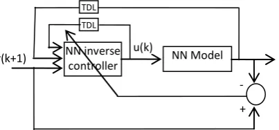
Inverse modeling plays a crucial role in IMC structure. The inverse learning structure is shown in Fig. 4. In this structure the plant model precedes the network to be trained as the inverse. We use the plant model because the plant is unknown. Using this architecture, we are able to explicitly calculate the partial derivatives of the plant model output with
respect to its input. From (2), the inverse function f1 leading to the generation of u(k) would require knowledge of the future value y(k1). To overcome this problem, we replace this future value with the value of the reference signal
) 1 k (
r , which we assume is available at time k . Thus, the nonlinear relation of the network modeling the plant inverse is given by ) 1) m -u(k , 1), -u(k 1), r(k 1), n -(k yˆ , ), k ( yˆ ( fˆ ) k ( u 1 (12)
[image:3.595.327.529.480.574.2]The condition governing the inevtibility of known system is that the linearization of the plant (1) around the equilibrium state is controllable.
Fig. 4: Plant model inverse modeling using neural networks.
The structure of inverse neural network is similar to that used for plant modeling. A multilayer network with an input layer, an output layer with one node, and two hidden layers is used to model the inverse model represented by (12).
The inverse multilayer network performs the calculations
i 1 h j c i 1 h ji 1 h j cj f w X b
I (13)
j 2 h r c j 2 h rj 2 h r cr f w I b
Z (14)
NN inverse
controller NN Model
TDL TDL ) 1 k ( yˆ
+ -+ u(k)
r o c r o r o b Z w f ) k (u (15)
where the input vector is given by
T T c m n c 1 c 0 c 1)) m -u(k , 1), -u(k 1), r(k 1), n -(k yˆ , ), k ( yˆ ( ) X , , X , X ( X (16)
The criterion to be minimized is given by:
2
c (r(k 1) yˆ(k 1))
2 1
J (17)
A recursive algorithm, used to adjust weights, is given by
w J ) k ( w ) 1 k ( w w J ) k ( w ) 1 k ( w w J ) k ( w ) 1 k ( w 1 h ji c 1 h ji 1 h ji 2 h rj c 2 h rj 2 h rj o r c o r o r (18) where 1 h ji c 1 h ji c 2 h rj c 2 h rj c o r c o r c w ) k ( u . ) k ( u ) 1 k ( yˆ . ) 1 k ( yˆ J w J w ) k ( u . ) k ( u ) 1 k ( yˆ . ) 1 k ( yˆ J w J w ) k ( u . ) k ( u ) 1 k ( yˆ . ) 1 k ( yˆ J w J (19) and )) 1 k ( yˆ ) 1 k ( r ( ) 1 k ( y ˆ Jc (20)
r j h1 ji c j c j h2 rj c r c r or. Z .(1- Z ). w .I .(1-I ).w
w ) k ( u ) 1 k ( yˆ (21)
r c i c j c j h2 rj c r c r o r 1 h ji c j c r c r o r 2 h rj c r o r X * ) I -(1 . I * w * ) Z -(1 . Z . w w ) k ( u I * ) Z -(1 . Z . w w ) k ( u Z w ) k ( u (22)The training process is continued until the control sequence leads to minimize the difference between the plant model and the reference signal.
6.
IMC CONTROLLER DESIGN
After training the plant neural network and inverse neural network models, as given in sections 4 and 5, we can incorporate them in the NN IMC structure given in section 3, Fig. 2.
Because plant neural network and inverse neural network models are implemented according to equations (11) and (12)
] 1) m -u(k , 1), -u(k u(k), 1), n -(k yˆ , 1), -(k yˆ ), k ( yˆ [ fˆ ) 1 k ( y ˆ ) 1) m -u(k , 1), -u(k 1), r(k 1), n -(k yˆ , ), k ( yˆ ( fˆ ) k ( u 1
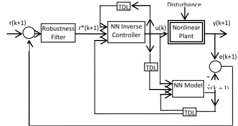
the block diagram given in Fig. 5 gives more details about the Internal Model Control structure.
[image:4.595.309.547.292.418.2]
Fig. 5: Detailed structure of Internal Model Control
The difference between the nonlinear plant output and plant neural network model (internal model) output represents the effect of disturbances and internal model mismatch.
If the NN inverse controller static gain is equal to the inverse of the internal model static gain and if the overall closed loop system is stable, this structure presents robustness properties against disturbances and modeling mismatch; it allows having an offset-free response by canceling the noise at the process output.
In practice perfect model cannot be obtained. In addition, the infinite gain required by perfect control would lead to sensitivity problem under model uncertainty.
A filter is usually added at the input of the NN inverse controller to attenuate uncertainties in the feedback, generated by the difference between plant and model outputs and serves to moderate excessive control effort. In [11] it was found that to ensure robust stability, whether the model order, it is always possible to use first order filter of the form
)] 1 k ( e ) 1 k ( r [ z 1 z ) 1 ( ) 1 k ( r 1 1 *
(23)
where is the filter tuning parameter and r*(k1) is the
filter output. Robustness Filter NN Inverse Controller Nonlinear Plant NN Model y(k+1) e(k+1) r(k+1) u(k)
+
-
+
-Disturbance s TDL TDL TDL r*(k+1) ) 1 k (According to the Fig. 5, the models need to match, that is the inverse model should be the inverse of the forward model instead of the inverse of the system.
7.
SIMULATION RESULTS
This section demonstrates the application of the IMC strategy on the unknown nonaffine nonlinear systems for both tracking and disturbance rejection studies.
Example 1:
Consider the liquid level system described by the following equation [20]:
(k) x y(k)
0.3578u(k) 1)
-(k)u(k)u(k 0.1087x
(k) 0.04228x 1)
-(k)u(k (k)x 0.3084x
1) -0.1295u(k (k)
(k)x 0.03259x
1) -(k)u(k 0.1633x (k)u(k)
0.3103x
) 1 k ( u ) k ( x 3513 . 0 ) k ( x 9722 . 0 ) 1 k ( x
) k ( x ) 1 k ( x
2
1
2 1 1
2 1 2 2
1 2
2 2 2
2
2 1
(24)
The NARMAX model of the process should be written as:
1) -1)u(k)u(k
-0.1087y(k
) k ( u ) k ( y 3103 . 0 ) 1 k ( u ) k ( 0.3513y
) 1 k ( y ) k ( y 03259 . 0 1) -1)u(k -0.1633y(k
) 1 k ( y 04228 . 0 1) -1)u(k -y(k 0.3084y(k)
) 1 k ( u 1295 . 0 ) k ( u 3578 . 0 ) k ( y 9722 . 0 ) 1 k ( y
2
2 2
(25)
The control objective is to make the liquid level y(k1)to follow a desired trajectory
0.4 )) 50 k sign(sin( 3
. 0 ) 1 k (
r (26)
In order to explain the disturbance-rejection capabilities of the Internal model control (IMC) structure, additive noise plus the influence of unknown plant dynamics are considered. The following additive noise is assumed to corrupt the output:
)) sin(35.49t +
) sin(23.66t +
sin(12t) + (sin(8t) * 0.01
d(k) (27)
To control this unknown nonlinear plant, the control process is divided into the following steps:
Step 1: Plant modeling
Using random input signal uniformly distributed over the interval [1,1] and input/output patterns generated from the unknown plant, neural network model of the plant with 10 nodes in the 1st hidden layer and 5 neurons in the 2nd hidden layer can be trained using the rules given in section 4 to model the plant (24) represented by NARMAX model given by
] 1) -u(k u(k), 1), -y(k ), k ( y [ f ) 1 k (
y (28)
The initial network weight values are selected randomly from the interval [1,1] and the learning rate () used is equal 0.2. Fig. 6 shows the output of the plant and the output of the model for a randomly selected input signal uniformly distributed over the interval [1,1]. Fig. 7 shows the error between model and plant which proves the accuracy of the modeling process. So the neural network model is used to find neural network inverse controller.
Step 2: Using neural network plant model obtained from step 1 and the architecture given in Fig. 4, the neural network inverse controller represented by
] 1) -u(k 1), r(k ), 1 k ( y ), k ( y [ f ) k (
u 1 m m (29)
with 10 nodes in the 1st hidden layer and 5 neurons in the 2nd hidden layer can be obtained. The initial network weight values are selected randomly from the interval [1,1] and the learning rate () used is equal 0.08. The rules used for the learning process are given in section 5. Fig. 8 shows the relation between input to the controller and output of the model. It can be seen from Fig. 8 that the relation is linear, as desired. Fig. 9 shows the tracking capabilities of the IMC strategy when the desired trajectory is given by (26) and the using the first-order filter F of the form given by
1 1
z 5 . 0 1
z 5 . 0
F
(30)
Fig. 10 gives the error between the reference signal r(k1) and the plant output yp(k1) result when IMC strategy is
used for tracking. The control input for the system (24) obtained using IMC strategy is given in Fig. 11.
Fig. 12 shows the disturbance given by (27). Fig. 13 shows that the performance of the IMC structure is satisfactory when controlling the system subjected to disturbance given by (27). The error between the reference signal r(k1) and the plant output yp(k1), result when IMC strategy is used to control
system subjected to disturbance (27), is shown in Fig. 14.
-1.2 -1 -0.8 -0.6 -0.4 -0.2 0 0.2 0.4 0.6 0.8
0 50 100 150 200
k
Pl
a
n
t
a
n
d
N
N
m
o
d
e
l
o
u
tp
u
[image:5.595.319.536.481.739.2]ts
Fig. 6: Model and Plant response using random input uniformly distributed over the interval [1,1].
-0.015 -0.01 -0.005 0 0.005 0.01 0.015
0 50 100 150 200
k
e
(k
)
Fig. 7: Error between model and plant response when using random input uniformly distributed over the interval [1,1].
0.1 0.2 0.3 0.4 0.5 0.6 0.7
0.1 0.2 0.3 0.4 0.5 0.6 0.7
r(k +1)
ym
(k
+1
)
0 0.1 0.2 0.3 0.4 0.5 0.6 0.7 0.8
0 50 100 150 200
k
r(
k+
1)
&
yp
(k
+1
[image:6.595.61.276.74.156.2])
Fig. 9: IMC tracking performance without disturbance.
-0.5 -0.3 -0.1 0.1 0.3 0.5
0 50 100 150 200
k
e
rr
o
r
b
e
tw
e
e
n
r
(k
+
1
)
a
n
d
y
p
(k
+
1
)
Fig. 10: Error between reference signal and output of the system.
-1.5 -1 -0.5 0 0.5 1 1.5 2
0 50 100 150 200
k
u
(k
[image:6.595.59.276.177.396.2])
Fig. 11: Control signal for the system (24) in case of reference model (26) when using IMC strategy.
-0.05 -0.03 -0.01 0.01 0.03 0.05
0 50 100 150 200
k
d
(k
[image:6.595.58.277.429.632.2])
Fig. 12: Disturbance of the plant (24).
0 0.1 0.2 0.3 0.4 0.5 0.6 0.7 0.8
0 50 100 150 200
k
r(
k
+
1
)
&
yp
(k
+
1
[image:6.595.59.278.658.742.2])
Fig. 13 IMC tracking performance under disturbance (27).
-0.4 -0.3 -0.2 -0.1 0 0.1 0.2 0.3
0 50 100 150 200
k
e
(k
+
1
)
Fig. 14: Error between reference signal and output of the system when the system under disturbance (27).
Example 2:
Consider the first order SISO system as described in the following difference equation [13]:
)]) k ( u ) k ( y cos[ 5 )( k ( u )] k ( y sin[ ) 1 k (
y (31)
The objectives of simulations include the following:
1) Test the approximation performance of the NN input-output approximation model under the following test signal with amplitude.
25 k 2 sin 5 . 0 50
k 2 sin 5 . 0 ) k (
u (32)
2) Track the following trajectories with magnitude:
100 k 2 sin 2 50
k 2 sin 2 ) k (
r (33)
when using the neural network IMC strategy.
3) Explain the disturbance-rejection capabilities of the Internal model control (IMC) structure, additive noise plus the influence of unknown plant dynamics are considered. The following additive noise is assumed to corrupt the output:
d(k)0.01*(cos(3t)) (34)
To control this unknown nonlinear plant, the control process is divided into the following steps:
Step 1: Plant modeling
using random input signal uniformly distributed over the interval [1,1] and input/output patterns generated from the unknown plant, neural network model of the plant with 20 nodes in the 1st hidden layer and 11 neurons in the 2nd hidden layer can be trained as seen in section 4 to model the plant (31) represented by NARMAX model as given by
] u(k) , ) k ( y [ f ) 1 k (
y (35)
The initial network weight values are selected randomly from the interval [1,1] and the learning rate () used is equal
1 .
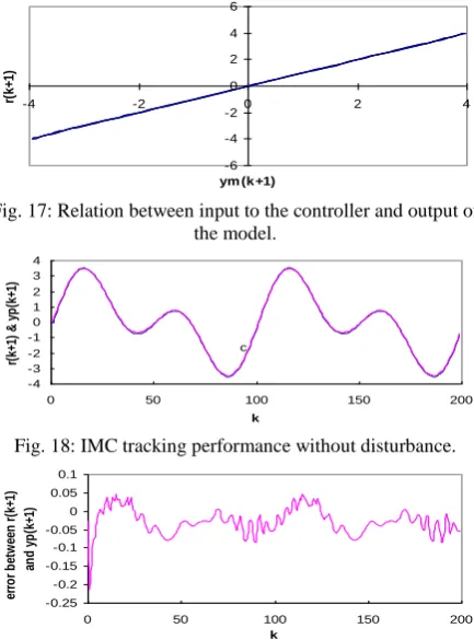
0 . Fig. 15 shows the output of the plant and the output of the model for a randomly selected input signal uniformly distributed over the interval [1,1]. Fig. 16 shows the error between model and plant which proves the accuracy of the modeling process. So the neural network model is used to find neural network inverse controller.
Step 2: Using neural network plant model obtained from step 1 and the architecture given in Fig. 4, the neural network inverse controller represented by
] 1) r(k ), k ( y [ f ) k (
u 1 m (36)
Fig. 19 gives the error between the reference signal r(k1) and the plant output yp(k1) result when IMC strategy is
used for tracking. The control input for the system (31) obtained using IMC strategy is given in Fig. 20.
Fig. 21 shows the disturbance given by (34). Fig. 22 shows that the performance of the IMC structure is satisfactory when controlling the system subjected to disturbance given by (34). The error between the reference signal r(k1) and the plant output yp(k1), result when IMC strategy is used to control
system (31) subjected to disturbance (34), is shown in Fig.23.
-6 -4 -2 0 2 4 6
0 50 100 150 200
k
yp
(k
+1
)
&
ym
(k
+1
[image:7.595.321.538.75.163.2])
Fig. 15: Model and Plant response using random input uniformly distributed over the interval [1,1].
-0.03 -0.02 -0.01 0 0.01 0.02
0 50 100 150 200
k
e(
k+
1)
Fig. 16: Error between model and plant response when using random input uniformly distributed over the interval [1,1].
-6 -4 -2 0 2 4 6
-4 -2 0 2 4
ym (k+1)
r(
k
+
1
[image:7.595.317.538.193.389.2])
Fig. 17: Relation between input to the controller and output of the model.
-4 -3 -2 -1 0 1 2 3 4
0 50 100 150 200
k
r(
k+
1)
&
yp
(k
+1
)
c
Fig. 18: IMC tracking performance without disturbance.
-0.25 -0.2 -0.15 -0.1 -0.05 0 0.05 0.1
0 50 100 150 200
k
er
ro
r
b
et
w
ee
n
r
(k
+1
)
an
d
y
p
(k
+1
)
Fig. 19: Error between reference signal and output of the system.
-1.5 -1 -0.5 0 0.5 1 1.5
0 50 100 150 200
k
u
(k
)
Fig. 20: Control signal for the system (31) in case of reference model (33) when using IMC strategy.
-0.015 -0.01 -0.005 0 0.005 0.01 0.015
0 50 100 150 200
k
d
(k
)
Fig. 21: Disturbance of the plant (31).
-5 -4 -3 -2 -1 0 1 2 3 4
0 50 100 150 200
k
r(
k
+
1
)
&
yp
(k
+
1
)
Fig. 22: IMC tracking performance when the system is under disturbance (34).
-0.6 -0.4 -0.2 0 0.2 0.4 0.6
0 100 200 300 400 500
k
e
(k
+
1
)
Fig. 23: Error between reference signal and output of the
system when the system is under disturbance (34).
8.
COMPARISON STUDY
In this section, we will make a comparison between two control cases 1) when nonaffine nonlinear discrete-time systems are subject to disturbances and 2) when nonaffine nonlinear discrete-time systems are without any disturbances. Related to example 1, Mean square error, between the reference model r(k1) and the plant output yp(k1), in
the first case is given by 4.8103 and in the second case is
given by 3103. Related to example 2, Mean square error, between the reference model r(k1) and the plant output
) 1 k (
yp , in the first case is given by 1.2102 and in the
[image:7.595.59.275.206.389.2] [image:7.595.59.276.431.724.2]9.
CONCLUSION
This paper described the use of nonlinear internal model control (IMC), based on two feedforward neural networks, to control unknown nonaffine nonlinear systems. The neural network models (internal model and inverse model) are obtained from input-output data using a three-layer feedforward network trained with a backpropagation algorithm. The nonlinear IMC controller consists of a model inverse controller and a robustness filter with a single tuning parameter. Simulation results for two unknown nonaffine nonlinear systems demonstrate the ability of the IMC strategy to perform tracking control. In view of the flexibility that neural networks provide in modeling unknown nonlinear systems, the nonlinear IMC is potentially applicable to control unknown nonaffine nonlinear systems subjected under external disturbances.
10.
ACKNOWLEDGEMENT
The author would like to thank King Saud University for its academic and financial support throughout the research work.
11.
REFERENCES
[1] Adetona O., Sathananthan S. and Keel L. H. 2004. Robust adaptive control of nonaffine nonlinear plants with small input signal changes. IEEE Trans. Neural Networks, l5(2), 408-416.
[2] Awais M. M. 2005. Application of internal model control methods to industrial combustion. Applied Soft Computing. 5, 223-233.
[3] Carotenuto R. 2001. An iterative system inversion technique. International Journal of Adaptive Control and Signal Processing. 15, 85-91.
[4] Chidrawar S. K. and Patre B. M. 2008. Implementation of neural network for internal model control and adaptive control. International Conference on Computer and Communication Engineering. Kuala Lumpur, Malaysia.
[5] Colin G., Chamaillard Y., Bloch G. and Corde G. 2007. Neural control of fast nonlinear systems application to a turbocharged SI engine with VCT. IEEE Trans. Neural Networks, l8(4), 1101-1114.
[6] Economou, C. G., Morari, M., and Palsson, B. O. 1986. Internal model control. 5. Extension to nonlinear systems. Ind. Eng. Chem. Press Des. Dev., 25, 403-411.
[7] Haykin, S., 1999. Neural networks. Printice-Hall.
[8] Hornik K, Stincheombe M and White H. 1989. Multilayer feedforwaed networks are universal approximators. Neural Networks, 2, 359-366.
[9] Li H. X. and Deng H. 2006. An approximate internal model based neural network control for unknown nonlinear discrete time systems. IEEE Trans. Neural Networks, l7(3), 659-670.
[10] Lightbody, G., and Irwin, G. W. 1997. Nonlinear control structures based on embedded neural system models. IEEE Trans. Neural Networks, 8(3), 553-567.
[11] Morari M. and Zafiriou E. 1989. Robust process control. Prentice-Hall, Englewood cliffs, NJ.
[12] Nahas, E. P., Henson, M. A., and Seborg, D. E. 1992. Nonlinear internal model control strategy for neural network models. Computa. Chem. Eng., 16(12), 1039-1057.
[13] Narendra K. S. and Mukhopadhyay S. 1997. Adaptive control using neural networks and approximate models. IEEE Trans. Neural Networks, 8, 475-485.
[14] Narendra K. S. and Parthasarathy K., 1990. Identification and control of dynamical systems using neural networks. IEEE Trans. Neural Networks, l(1), 4-27.
[15] Norgaard, M., Ravan, O., Poulsen N. K., and Hansen L. K. 2000. Neural networks for modeling and control of dynamical systems. London, U. K.:Spring-Verlag.
[16] Noriega J. R. and Wang H. 1998. A direct adaptive neural-network control for unknown nonlinear systems and its applications. IEEE Trans. Neural Networks, 9(1), 27-34.
[17] Plett G. L. 2003. Adaptive inverse control of linear and nonlinear systems using dynamic neural networks. IEEE Trans. Neural Networks, 14(2), 360-376.
[18] Rivals, I., and Personnaz, L. Nonlinear internal model control using neural networks: Applications to processes with delay and design issues. IEEE Trans. Neural Networks, 11(1), 80-90.
[19] Yang Q., Vance J. B. and Jagannathan S. 2008. Control of nonlinear discrete-time systems using reinforcement learning based linearly parameterized neural networks. IEEE Trans. Neural Networks, 38(4), 994-1001.
[20] Zhai L. F., Chai T. Y. and Ge S. S. 2007. Stable adaptive neural network control of nonaffine nonlinear discrete-time systems and application. 22th IEEE International Symposium on Intelligent Control, Singapore. 602-607.
![Fig. 6: Model and Plant response using random input uniformly distributed over the interval []1 ,1](https://thumb-us.123doks.com/thumbv2/123dok_us/8123496.794854/5.595.319.536.481.739/model-plant-response-using-random-uniformly-distributed-interval.webp)