An Improved Q-learning Algorithm for Path-Planning of a
Mobile Robot
Pradipta K Das
1, S. C. Mandhata
2, H.S Behera
3, S.N. Patro
41,2,4
Dhaneswar Rath Institue of Engineering & Management Studies Cuttack-754022, India
3
VSSUT, Burla-768018 Odisha, India
ABSTRACT
Classical Q-learning requires huge computations to attain convergence and a large storage to save the Q-values for all possible actions in a given state. This paper proposes an alternative approach to Q-learning to reduce the convergence time without using the optimal path from a random starting state of a final goal state, when the Q-table is used for path planning of a mobile robot. Further, the proposed algorithm stores the Q-value for the best possible action at a state, and thus save significant storage. Experiments reveal that the acquired Q-table obtained by the proposed algorithm helps in saving turning angles of the robot in the planning stage. Reduction in turning angles is economic from the point of view of energy consumption by the robot. Thus the proposed algorithm has several merits with respect to classical Q-learning. The proposed algorithm is constructed based on four fundamental properties derived here and the validation of the algorithm is studied with Khepera-II robot.
Keywords:
Q-learning; Reinforcement learning; Motion planning, Mobile Robot, Energy.1.INTRODUCTION
Machine learning is often used in mobile robots to make the robot aware about its world map. In early research on mobility management of robots, supervised learning was generally employed to train a robot to determine its next position in a given map from the sensory readings about the environment. Supervised learning is a good choice for mobility management of robots in fixed maps. However, if there is a small change in the robot’s world, the acquired knowledge is no longer useful to guide the robot to select its next position. A complete training of the robot with both old and new sensory data-action pairs is then needed to overcome the said problem.
Reinforcement learning is an alternative learning policy, which rests on the principle reward and punishment. No prior training instances are presumed in reinforcement learning. A learning agent here does an action on the environment, and receives a feedback from the environment based on its action. The feedback provides an immediate reward for the agent. The learning agent here usually adapts its parameter based on the current and cumulative (futuristic) rewards. Since the exact value of the futuristic reward is not known, it is guessed from the knowledge about the robot’s world map. The primary advantage of reinforcement learning lies in its inherent power of automatic learning even in presence of small changes in the world map. Motion planning is one of the important tasks in intelligent control of a mobile robot. The problem of motion planning is often decomposed into path planning and trajectory planning. In path planning, we need to generate a collision-free path in an environment with obstacles and optimize it with respect to some
criterion [8], [9]. However, the environment may be imprecise, vast, dynamical and partially non-structured [7]. In such environment, path planning depends on the sensory information of the environment, which might be associated with imprecision and uncertainty. Thus, to have a suitable planning scheme in a cluttered environment, the controller of such kind of robots must have to be adaptive in nature. Trajectory planning, on the other hand, considers time and velocity of the robots, while planning its motion to a goal. It is important to note that path planning may ignore the information about time/velocity, and mainly considers path length as the optimality criterion. Several approaches have been proposed to address the problem of motion planning of a mobile robot. If the environment is a known static terrain and it generates a path in advance, it is said to be off-line algorithm. It is called on-line, if it is capable of producing a new path in response to environmental changes.
Many studies have been carried out on path planning for different types of mobile robots. The works in [5] involve mapping, navigation, and planning tasks for Khepera II mobile robot. In these works, the computationally intensive tasks, such as the planning and mapping tasks were not performed onboard. They were performed on a separate computer. The sensor readings and the motor commands are communicated between the robot and the computer via serial connection.
Usually, the planning involves an action policy to reach a desired goal state, through maximization of a value function [1]-[3], which designates sub-objectives and helps choosing the best path. For instance, the value function could be the shortest path, the path with the shortest time, the safest path, or any combination of different sub-objectives. The definition of a task in this class may contain, besides the value function, some a priori knowledge about the domain, e.g., environmental map, environmental dynamics, goal position. Such knowledge allows a robot planning, while the lack of such knowledge obliges the robot either to learn it previously or to make use of heuristic strategies, such as moving to goal direction while avoiding obstacles. Our research applies reinforcement learning techniques to real-world robots. Reinforcement learning has been tested in many simulated environments [3]- [11] but on a limited basis in real-world scenarios. A real-real-world environment poses more challenges than a simulated environment, such as enlarged state spaces [2], increased computational complexity, significant safety issues (a real robot can cause real damage), and longer turnaround times for results. This research measures how well reinforcement-learning technique, such as Q-learning, can apply to the real robot for navigational problem, and in our research we modified the classical Q-learning algorithm, hereafter called improved Q-learning for increasing its performance one in the path-planning problem.
learn the changed environment again. This problem is overcome in the algorithm proposed here. In the Extended Q-learning, sometime the robot needs more energy because the robot needs to rotate in selecting the best action. In the newly proposed algorithm, this problem is rectified.
The rest of the paper is organized as follows. Classical learning is introduced in section II. Some properties of the Q-learning based on the concept of locking of states are derived in section III. The algorithm for the Improved Q-learning is given in section IV. The algorithm for the path planning is given in section V. Computer Simulation is shown in section VI. Experimental details are included in section VII. Conclusions are listed in section VIII.
2.THE
CLASSICAL
Q-LEARNING
In classical Q-learning, all possible states of an agent and its possible action in a given state are deterministically known. In other words, for a given agent A, let S0, S1, S2, ..., Sn, be n- possible states, where each state has m possible actions
a
0,
,
1
a
a
2,
...,a
m. At a particular state-action pair, the specific reward that the agent acquires is known as immediate reward. For example r(Si,a
j) denotes the immediate reward that the agent A acquires by executing an actiona
j at state Si. An agent selects its next state from its current states by using a policy. This policy attempts to maximize the cumulative reward that the agent could have in subsequent transition of states from its next state. For example, let the agent be in state Si and is expecting to select the next best state. Then the Q-value at state Si due to action ofa
j is given in (1).Q(S, ) r(S , ) ( ( , ), /)
j i j
i a a Max/ Q Si aj a
a
(1)
where (Si,
a
j) denotes the next state due to selection of actionj
a
at state Si. Let the next state selected be Sk. Then Q( (Si ,a
j ),a
/) = Q(Sk,/
a
). Consequently selection ofa
/ that maximizing Q(Si,a
j) is an interesting problem. One main drawback for the above Q-learning is to know the Q-value at a state Sk for all possible action/
a
. As a result, each time it accesses the memory to get Q-value for all possible actions at a particular state to determine the most appropriate next state. So it consumes more time to select the next state. Since the actiona
/ for which Q(Sk,/
a
) is maximum needs to be evaluated, we can remodel the Q-learning equation by identifying thea
/ that moves the agent closer to the goal.In the proposed Improved Q-learning, we have only one field for storing the Q-value and one for storing lock variable of the particular state. In this way the space requirement for storing the Q-table gets reduce.
3.
PROPERTIES
OF
THE
IMPROVED
Q-LEARNING
respectively. Let the distance in order be dbG <daG <dcG <ddG . Then the agent should select the next state Sb from its current state Sk. If the Q-value of the state Sb is known. We can evaluate the Q-value of state Sk by the following approach.
).
,
Q(S
γ
0
)
,
Q(S
(3)
:
have
we
(3)
and
(2)
Combining
)
d
(
).
,
Q(S
}
,
S
|
S
|
S
|
Q{S
M ax
)
),
,
(
(
Therefore,
operator.
OR
denotes
|
where
,
S
|
S
|
S
|
S
)
,
(S
δ
Now
(2)
)
),
,
S
(
(
Q
M ax
γ
0
)
),
,
(
(
)
,
(
)
,
(
// b / k aG // b // d c b // / d c b / k // / k // / / / // // // //a
a
d
d
d
a
a
a
a
S
Q
Max
a
a
a
a
a
S
Q
Max
a
S
r
a
S
Q
dG cG bG a a k a a a k a k k
Thus if the next state having the shortage distance with the goal is known, and the value of this state is also known, then the Q-value of the current state is simply ×Q-value of the next state. Let Sp, Sn and SG be the present, next and the goal states respectively. Let Qp and Qn be the Q-value at the present and the next states Sp and Sn respectively. Let dxy be the city block distance between the states Sx and Sy. We use a Boolean variable Lock: Lx to indicate that the Qx value of a state is fixed permanently. We set lock Ln=1 if the Q-value of the state n is fixed, and won’t change further after Ln is set to 1. The Lock variable for all states except the goal will be initialized zero in our proposed Q-learning algorithm. We observe four interesting properties as indicated below.
Property 1: If Ln=1 and dpG < dnG then Qp γQnand set
Lp = 1.
Proof. Let the neighborhood state of Sp be S
{Sa ,Sb,Sc ,Sn}, and the agent selects Sn as the next state as dnG < dxG for}.
,
,
,
{
a
b
c
n
x
Now,
) , (S QpQ p a
r(S
p,
)
γ
Q
δ
S
p
),
/
/
a
a
Max
a
a)
,
S
|
S
|
S
|
Q(S
γ
0
/ n c b a /a
Max
a
γ
Q
(S
n,
a
/)
(
d
nG
d
xG for})
,
,
,
{
a
b
c
n
x
=
γ
Q
n. Since Ln =1, and dpGdnG,
Q
p
Q
n,
and thusn
Q
γ
Q
p
for0
1
is the largest possible value ofp
Q
, andQ
pshould not be updated further. So, Lp = 1 is set.Property 2: If Ln=0 and dpGdnGthen γ
Proof. Let the neighborhood state of Sp be S
{Sa , Sb,Sc,Sn }, and the agent selects Sn as the next state as dnG dxG for}.
,
,
,
{
a
b
c
n
x
Now,
) , (S QpQ p a
r(S
p,
)
γ
Q
δ
S
p
),
/
/
a
a
Max
a
a
0
γ
Q(S
a|
S
b|
S
c|
S
n,
/)
/
a
Max
a
γ
Q
(S
n,
a
/)
(
d
nG
d
xGfor
x
{
a
,
b
,
c
,
n
})
γ
Q
n. (4)Since
nG
pG d
d ,
Q
p
Q
n.
So, Qp
Qnis logically satisfied. However, as Ln=0, Qn is not yet stable at the current iteration. So, Qp is also not stable yet. Let t be the current iteration. ThenQ (t) Q(t) n
p
if Qp(t1)
Qn(t). Q (t1),p otherwise.
The two alternatives in (5) can be put together as in (6). Qp(t) Max(Qp(t1),
Qn(t)) (6) Ignoring the notion of time t from (6), we obtain) , ( )
( p n
p t MaxQ Q
Q
.
Property 3: If Lp = 1 and dnGdpGthen Qn γQpand set Ln = 1.
Proof.Let the neighborhood of the next state Sn be S
{Sa ,Sb ,Sc ,Sp }. Since dpGdxG forx
{
a
,
b
,
c
,
p
}
, the agent will select the state Sp during its transition form Sn.Now,
Q
n
Q
(
S
n,
a
)
(
,
)
Q(S
a|
S
b|
S
c|
S
p,
/)
/
a
Max
a
S
r
a
n
0
γ
Q(S
a|
S
b|
S
c|
S
p,
/)
/
a
Max
a
γ
Q
(S
p,
a
/)
(
d
pG
d
xG,
x
).
p Q γ
.
Since dnGdpG, QnQp.So,
p
n Q
Q
is logically acceptable for0
1
. Further, as Lp=1, and Sn is the nearest state to Sp with respect to given distance metric, therefore Ln is set to 1.
Property 4: If Lp=0 and dnGdpGthen
). Q γ , Max(Q Qn n p
Proof. Let the neighborhood of state Sn be S
{Sa, Sb,Sc,Sp}. LetxG
pG d
d for
x
{
a
,
b
,
c
,
p
}.
Then the agent will select Sp during its transition from Sn,Now, QnQ(Sn,a)
(
,
)
Q(
(S
,
)
,
/)
n
/
a
a
Max
a
S
r
a
n
(
,
)
Q(S
|
S
|
S
|
S
,
/)
p c b a/
a
Max
a
S
r
a
n
0 γ Q(S, /) p a
(dpGdxG,x)
γQp.
Since dnGdpG,
QnQp.So,p
n Q
Q
for0
1
is logically satisfactory. Now, as Lp=0, Qp is not fixed until this iteration; So Qn is also not fixed in the current iteration. Now, adding the notion of iteration t in Qn and Qp, we have;Q(t) Q (t), p
n if Qn(t1)Qp(t), Qn(t1),otherwise.
Combining the expressions under (7) by a single expression, we write:
Qn(t)Max(Qn(t1),
Qp(t)) (8)Now, eliminating t from both sides of (8), we obtain,
QnMax(Qn,
Qp). (9)4.
THE
IMPROVED
Q-LEARNING
ALGORITHM
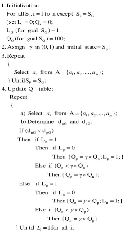
In the new Q-learning algorithm to be proposed, only two fields for each grid are required, one is used to store Q-value and other is used to store the Lock variable. In the new algorithm every state stored only the Q-value and not the best action to reach the goal state. The best path between the current state to the goal is given by the city-block distance; therefore there will be more than one best path to reach the goal. As a result selection of the best action is deferred till the path planning by doing so the energy required by the robot can be minimized. The newly proposed algorithm has four steps. Initialization of Q-table is done in step 1, in step 2, value of
and starting state of the robot are initialized. Q-table is updating only after the robot reaches the goal state for the first time. Thus the robot is allowed to come to the goal state without updating Q-table. This is done in step 3. The updating of the Q-table is done in step 4 using the properties introduced in section III.Pseudo Code for Improved Q-learning i; all for 1 Un til } } Q {Q Then ) Q (Q if Else } 1; L ; Q {Q Then 0 L if Then 1 L if Else }; Q γ Q { Then ) Q γ (Q if Else } 1; L ; Q γ {Q Then 0 L if Then 1 L if Then ) d (d If ; d and d Determine b) }; ..., , , { A from Select a) { Rep eat : table Q Up date 4. ; S S Until } }; ..., , , { A from Select { Rep eat 3. ; S state initial and 1) (0, in Assign γ 2. 100; ) S goal (for Q 1; ) S goal (for L 0; Q 0; L {set S S excep t n to 1 i , S all For tion Initializa . 1 p n p n n p n n p n p n p p n p p n pG nG pG nG 2 1 G P 2 1 p G G G G i i G i i i m i m i L a a a a a a a a
Space-Complexity: In classical Q-learning, if there are n states and m action per state, then the Q-table will be of (mn) dimension. In the Improved Q-learning, for each state 2 storages are required, one for storing Q-value and other for storing value of the lock variable of a particular state. Thus for n number of states, we require a Q-table of (2n) dimension. The saving in memory in the present context with respect to classical Q thus is given by mn 2n = n(m 2).
Time-Complexity: In classical learning, the updating of Q-values in a given state requires determining the largest Q-value, in that cell for all possible actions. Thus if there are m possible actions at a given state, maximization of m possible Q-values, require m 1 comparison. Consequently, if we have n states, the updating of Q values of the entire Q table by classical method requires n(m 1) comparisons. Unlike the classical case, here we do not require any such comparison to evaluate the Q values at a state Sp from the next state Sn. But we need to know whether state n is locked i.e., Q-value of Sn is permanent and stable. Thus if we have n number of states, we require n number of comparison. Consequently, we save n(m 1) n = nm 2n= n(m2).
5. PATH PLANNING
ALGORITHM
[image:4.595.53.255.90.463.2]action is selected by comparing the Q-value of the 4-neighbour states. If there are more than one state with equal Q-value than the action that requires minimum energy for turning is selected.
Fig. 1: Portion of environment with Q-value and robot at center.
In Fig. 1 the robot is at the centre facing toward east. Next feasible states are the 4-neighbour states and corresponding Q-value are given in each state. There are two states with maximum Q-value of 88. If the next state is located at south then the robot has to rotate toward right by 900 and if the next state is located at west then the robot has to rotate by 1800. Therefore, the presumed next state will be the state at south as the robot requires less energy to move to that state. During path planning the robot selects one out of several best actions at a given state. If an obstacle is present in the selected direction then next optimal path is selected. If there is no action to be selected then a signal is passed to the robot to backtrack one step.
Pseudo Code for Path Planning
END GOAL NEXT NEXT CURRENT NEXT NEXT CURRENT NEXT NEXT state starting CURRENT BEGIN ; until 2 step from Repeat 5. ; 4. ; to Go 3. free; -Obstacle is and of ood neighbourh the in value -Q the of value -Q where , state next Get 2. ; 1.
6.
COMPUTER
SIMULATION
We designed an environment of 20×20 grids. Every grid is given a state number. For a state at (x, y),
(10)
where x is the no of block in x direction y is the no of block in y direction
is the length of the row
We make the agent learn the environment with the proposed new algorithm and the original classical Q-learning algorithm for verifying the applicability of the proposed algorithm. We stop the classical Q-learning after 50 thousand iterations. For the new algorithm we allow to learn till all the Lock variables are set. Total numbers of iteration varies from 11 thousand to nearly 25 thousand as the position of the goal changes. Learning is done without any obstacle. After completion of learning we have kept the agent, facing left, in different environments and allow traversing to the goal using the stored Q-table by both the algorithm. The results are shown in the Fig. 2-Fig. 6 and Table 1.
87
7
86
85
86
87
88
89 88
Path taken by the robot with stored Q-table by Classical Q-learning Path taken by the robot with stored Q-table by Improved Q-learning
Figure 2: Environment 1 without obstacle.
Obstacle
Path taken by the robot with stored Q-table by Classical Q-learning Path taken by the robot with stored Q-table by Improved Q-learning
Figure 3: Environment 2 with obstacles.
Obstacle
[image:5.595.62.284.69.309.2]Path taken by the robot with stored Q-table by Classical Q-learning Path taken by the robot with stored Q-table by Improved Q-learning
Fig. 4: Environment 3 with obstacles.
TABLE I. COMPARISON OF TIME TAKEN BY THE ROBOT AND NO. OF 900 TURN REQUIRED BY THE ROBOTINDIFFERENTENVIRONMENTBYCLASSICAL Q-LEARNING (CQL) AND IMPROVED Q-LEARNING (IQL)
S.No Environment Time Taken in sec No. of 90
0 Turn
IQL CQL IQL CQL
1 1 22.13 25.65 1 19 2 2 30.98 35.32 17 25 3 3 32.35 66.40 24 70 4 4 17.85 32.24 10 27 5 5 22.85 33.72 11 31
Obstacle
[image:5.595.311.537.369.695.2]Path taken by the robot with stored Q-table by Classical Q-learning Path taken by the robot with stored Q-table by Improved Q-learning
Fig. 5: Environment 4 with obstacles.
S
G
S
G
S
G
S
Obstacle
[image:6.595.62.283.67.311.2]Path taken by the robot with stored Q-table by Classical Q-learning Path taken by the robot with stored Q-table by Improved Q-learning
Fig. 6: Environment 5 with obstacles.
7.EXPERIMENTS
WITH
KHEPERA
II
ROBOT
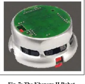
Khepera II (Figure 7) is a miniature robot (diameter of 8 cm) equipped with 8 built-in infrared range and light sensors, and 2 relatively accurate encoders for the two motors. The range sensors are positioned at fixed angles and have limited range detection capabilities. We numbered the sensors clockwise from the leftmost sensor to be sensor 0 to sensor 7(Figure 8). Sensor values are numerical ranging from 0 (for distance > 5 cm) to 1023 (approximately 2 cm).The onboard Microprocessor has a flash memory size of 256KB, and the CPU of 8 MHz. Khepera can be used on a desk, connected to a workstation through a wired serial link. This configuration allows an optional experimental configuration with everything at hand: the robot, the environment and the host computer.
Fig. 7: The Khepera II Robot
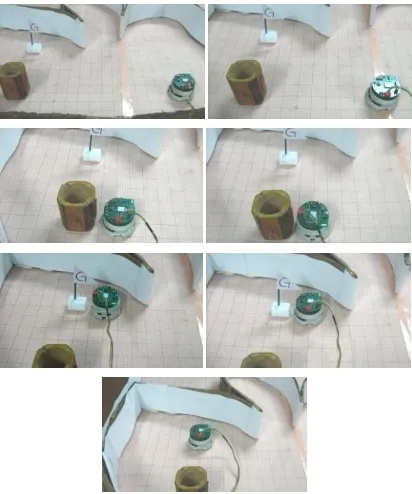
[image:6.595.352.490.73.198.2] [image:6.595.316.533.371.498.2]Experimental world map with and without obstacle is shown in Fig 9 and Fig 10. The Improved Q-learning algorithm is used in the first phase to learn the movement steps from each grid in the map to its neighbor. After the learning phase is over, the path planning algorithm is executed. The snapshots with and without obstacles are indicated in Fig. 11 and Fig. 12 respectively.
Fig. 8: Position of the sensors of Khepera II
Fig. 9. Experimental world map without obstacle.
Fig. 10. Experimental world map with obstacle.
Fig. 11. Snapshots of experimental planning (without
S
[image:6.595.103.246.508.649.2] [image:6.595.319.527.523.702.2]Fig. 12. Snapshots of experimental planning (with one
obstacle) instances in order.
8. CONCLUSIONS
The paper proposes a novel approach to reduce both time – and space-complexity of the Classical Q-learning algorithm. A mathematical foundation of the proposed algorithm indicates the correctness, and the experiments on simulated and real platform validate without losing the optimal path in path-planning applications of a mobile robot. The algorithm is coded in C-language and tested on IBM Pentium based simulation environment. The field study is performed on Khepera-II platform. Simulation results also confirm less number of 900 turning of the robot around its z-axis with respect to classical Q-learning, and the proposed algorithm helps in energy saving of the robot in path-planning application.
9. REFERENCES
[1] Dean, T., Basye, K. and Shewchuk, J. “Reinforcement learning for planning and Control”. In: Minton, S. (ed.) Machine Learning Methods for Planning and Scheduling. Morgan Kaufmann 1993.
[2] Bellman, R.E., “Dynamic programming “, Princeton, NJ: Princeton University Press, p. 957.
[3] Watkins, C. and Dayan, P., “Q-learning,” Machine Learning, Vol. 8, pp. 279- 292, 1992
[4] Konar, A., Computational Intelligence: Principles, Techniques and Applications. Springer-Verlag, 2005 [5] Busoniu, L., Babushka, R., Schutter, B.De., Ernst, D.,
Reinforcement Learning and Dynamic Programming Using
Function Approximators, CRC Press, Taylor & Francis group, Boca Raton, FL, 2010.
[6] Chakraborty, J., Konar A., Jain, L.C., and Chakraborty, U., “Cooperative Multi-Robot Path Planning Using Differential Evolution” Journal of Intelligent & Fuzzy Systems, Vol. 20, Pp.13-27, 2009.
[7] Gerke, M., and Hoyer, H., Planning of Optimal paths for autonomous agents moving in inhomogeneous environments, in: Proceedings of the 8th Int. Conf. on Advanced Robotics, July 1997, pp.347-352.
[8] Xiao, J., Michalewicz, Z., Zhang, L., and Trojanowski, K., Adaptive Evolutionary Planner/ Navigator for Mobile robots, IEEE Transactions on evolutionary Computation 1 (1), April 1997.
[9] Bien, Z., and Lee, J., A Minimum–Time trajectory planning Method for Two Robots, IEEE Trans on Robotics and Automation 8(3).PP.443-450, JUNE 1992.
[10] Moll, M., and Kavraki, L.E., Path Planning for minimal Energy Curves of Constant Length, in: Proceedings of the 2004 IEEE Int. Conf. on Robotics and Automation, pp.2826-2831, April 2004.
[11] Regele, R., and Levi, P., Cooperative Multi-Robot Path Planning by Heuristic Priority Adjustment, in: Proceedings of the IEEE/RSJ Int Conf on Intelligent Robots and Systems, 2006.
[12] Yuan-Pao Hsu, Wei-Cheng Jiang, Hsin-Yi Lin, A CMAC-Q-Learning Based Dyna Agent, in: SICE Annual Conference, 2008, pp. 2946 – 2950, The University Electro-Communications, Tokyo, Japan.
[13] Yi Zhou and Meng Joo Er, A Novel Q-Learning Approach with Continuous States and Actions, in: 16th IEEE International Conference on Control Applications Part of IEEE Multi-conference on Systems and Control, Singapore, 1-3 October 2007
[14] Kyungeun Cho, Yunsick Sung, Kyhyun Um, A Production Technique for a Q-table with an Influence Map for Speeding up Q-learning, in : International Conference on Intelligent Pervasive Computing, 2007.
[15] Deepshikha Pandey, Punit Pandey, Approximate Q-Learning: An Introduction, in : Second International Conference on Machine Learning and Computing, 2010. [16] S. S. Masoumzadeh and G. Taghizadeh, K. Meshgi and S.
Shiry, Deep Blue: A Fuzzy Q-Learning Enhanced Active Queue Management Scheme, in : International Conference on Adaptive and Intelligent Systems, 2009.