R E S E A R C H
Open Access
An alternative extragradient projection
method for quasi-equilibrium problems
Haibin Chen
1*, Yiju Wang
1and Yi Xu
2*Correspondence:
[email protected] 1School of Management Science,
Qufu Normal University, Rizhao Shandong, China
Full list of author information is available at the end of the article
Abstract
For the quasi-equilibrium problem where the players’ costs and their strategies both depend on the rival’s decisions, an alternative extragradient projection method for solving it is designed. Different from the classical extragradient projection method whose generated sequence has the contraction property with respect to the solution set, the newly designed method possesses an expansion property with respect to a given initial point. The global convergence of the method is established under the assumptions of pseudomonotonicity of the equilibrium function and of continuity of the underlying multi-valued mapping. Furthermore, we show that the generated sequence converges to the nearest point in the solution set to the initial point. Numerical experiments show the efficiency of the method.
MSC: 90C30; 15A06
Keywords: Quasi-equilibrium problems; Extragradient projection method; Pseudomonotonicity; Multi-valued mapping
1 Introduction
The equilibrium problem has been considered as an important and general framework for describing various problems arising in different areas of mathematics, including op-timization problems, mathematical economic problems and Nash equilibrium problems. As far as we know, this formulation has been followed for a long time by several studies on equilibrium problems considered under different headings such as quasi-equilibrium problem, mixed equilibrium problem, ordered equilibrium problem, vector equilibrium problem and so on [1–4]. It should be noted that one of the interests of this common for-mulation is that many techniques developed for a particular case may be extended, with suitable adaptations, to the equilibrium problem, and then they can be applied to other particular cases [5–16]. In this paper, we mainly deal with existence of solutions and ap-proximate solutions of the quasi-equilibrium problem.
Let X⊂Rn be a nonempty closed convex set,K be a point-to-set mapping from X
that
fx∗,y≥0, ∀y∈Kx∗. (1.1)
Throughout this paper, we denote the solution set byK∗.
Certainly, whenf(x,y) =F(x),y–x withFbeing a vector-valued mapping fromXto Rn, then the quasi-equilibrium problem reduces to the generalized variational inequality
or quasi-variational inequality problem [17–20] which is to find vectorx∗∈K(x∗) such that
Fx∗,y–x∗≥0, ∀y∈Kx∗. (1.2)
To move on, we recall the classical equilibrium problem, and classical Nash equilibrium problem (NEP) [21]. Assume the function fi:Rn→Ris continuous, and supposeKiis
a nonempty closed set inRni fori= 1, 2, . . . ,N withn=N
i=1ni. Suppose that there are N players such that each player controls the variablesxi∈Rni. Denote x= (x1, . . . ,xN),
andx–i= (x1, . . . ,xi–1,xi+1, . . . ,xN). Playerineeds to take anxi∈Ki⊂Rni that solves the
following optimization problem:
min xi∈Ki
fi(xi,x–i)
based on the other players’ strategiesx–i. If theseNplayers do not cooperate, then each
players’ strategy set may vary with other players’ strategies, that is, theith player’s strategy set varies with the other players’ strategiesx–i. In this case, we need to useKi(x–i) instead
ofKito indicate theith player’s strategy set, and theith player needs to choose a strategy x∗i ∈Ki(x–i) that solves the following optimization problem:
min xi∈Ki(x–i)
fi(xi,x–i).
In [22], the non-cooperative game model is called generalized Nash equilibrium problem (GNEP), which can be formulated as the quasi-equilibrium problem where the involved functions are nondifferentiable [23].
For the problem GNEP, when the functionsfi(·,x–i) are convex and differentiable, then
the problem can be equivalently formulated as the quasi-variational inequalities (1.2) by setting
F(x) =∇xifi(x) N
i=1
andK(x) =Ni=1Ki(x–i). When the functionfi(·,x–i) is convex and nondifferentiable, then
the GNEP reduces to the quasi-equilibrium problem (1.1) [24] via the Nikaido Isoda fun-tion
f(x,y) =
N
i=1
fi(yi,x–i) –fi(xi,x–i)
.
more information see [19, 25, 26]. There are many solution methods for solving QEP. Re-cently, [27] considered an optimization reformulation approach with the regularized gap function. Different from the variational inequalities problem, the regularized gap function is in general not differentiable, but only directional differentiable. Furthermore, supple-mentary conditions must be imposed to guarantee that any stationary point of these func-tions is a global minimum, since the gap funcfunc-tions is nonconvex [28]. It should be noted that such conditions are known for variational inequality problem but not for QEP. So, [23] proposed several projection and extragradient methods rather than methods based on gap functions, which generalized the double-projection methods for variational in-equality problem to equilibrium problems with a moving constraint setK(x).
It is well known that the extragradient projection method is an efficient solution method for variational inequalities due to its low memory and low cost of computing [29, 30]. Based on those advantages, it was extended to solve QEP recently [20, 23, 31] and this opened a new approach for solving the problem. An important feature of this method is that it has the contraction property in the sense that the generated sequence has contrac-tion property with respect to the solucontrac-tion set of the problem [29],i.e.
xk+1–x∗≤xk–x∗, ∀k≥0,x∗∈K∗.
The numerical experiments given in [20, 23, 31] show that the extragradient projection method is a practical solution method for the QEP.
It should be noted that not all the extragradient projection methods have the contrac-tion property [32]. In that case, it may not slow down the convergence rate significantly. Al-though the extragradient projection method has no contraction property, it still has a good numerical performance [32]. Now, a question can be posed naturally, can this method be applied to solve the QEP? And if so, how about its performance? This constitutes the main motivation of this paper.
Inspired by the work [23, 32], we propose a new type of extragradient projection method for the QEP in this paper. Different from the extragradient projection method proposed in [23], the generated sequence by the newly designed method possesses an expansion property with respect to the initial point,i.e.,
xk+1–xk2+xk–x02≤xk+1–x02.
The existence results for (1.1) are established under pseudomonotonicity condition of the equilibrium function and the continuity of the underlying multi-valued mapping. Further-more, we show that the generated sequence converges to the nearest point in the solution set to the initial point. Numerical experiments show the efficiency of the method.
2 Preliminaries
LetXbe a nonempty closed convex set inRn. For anyx∈Rn, the orthogonal projection
ofxontoXis defined as
y0=arg min
y–x |y∈X,
and denotePX(x) =y0. A basic property of the projection operator is as follows [33].
Lemma 2.1 Suppose X is a nonempty,closed and convex subset inRn.For any x,y∈Rn,
and z∈X,we have
(i) PX(x) –x,z–PX(x) ≥0;
(ii) PX(x) –PX(y)2≤ x–y2–PX(x) –x+y–PX(y)2.
Remark2.1 The first statement in Lemma 2.1 also provides a sufficient condition for
vec-tory∈Xto be the projection of vectorx,i.e.,y=PX(x) if and only if
y–x,z–y ≥0, ∀z∈X.
To proceed, we present the following definitions [34].
Definition 2.1 SupposeXis a nonempty subset ofRn. The bifunctionf :X×X→Ris
said to be
(i) strongly monotone onXwithβ> 0iff
f(x,y) +f(y,x)≤–βx–y2, ∀x,y∈X;
(ii) monotone onXiff
f(x,y) +f(y,x)≤0, ∀x,y∈X;
(iii) pseudomonotone onXiff
f(x,y)≥0 ⇒ f(y,x)≤0, ∀x,y∈X.
Definition 2.2 SupposeXis a nonempty, closed and convex subset ofRn. A multi-valued
mappingK:X→2Rnis said to be
(i) upper semicontinuous atx∈Xif for any convergent sequence{xk} ⊂Xwithx¯
being the limit, and for any convergent sequence{yk}withyk∈K(xk)and¯ybeing
the limit, then¯y∈K(x¯);
(ii) lower semicontinuous atx∈Xif given any sequence{xk}converging toxand any y∈K(x), there exists a sequence{yk}withyk∈K(xk)converges toy;
(iii) continuous atx∈Xif it is both upper semicontinuous and lower semicontinuous atx.
Assumption 2.1 For the closed convex setX⊂Rn, the bifunctionf and multi-valued
mappingKsatisfy:
(i) f(x,·)is convex for any fixedx∈X,f is continuous onX×Xandf(x,x) = 0for all
x∈X;
(ii) Kis continuous onXandK(x)is a nonempty closed convex subset ofXfor all
x∈X;
(iii) x∈K(x)for allx∈X;
(iv) S∗={x∈S|f(x,y)≥0,∀y∈T}is nonempty forS=x∈XK(x)andT=x∈XK(x); (v) f is pseudomonotone onXwith respect toS∗i.e.f(x∗,y)≥0⇒f(y,x∗)≤0,
∀x∗∈S∗,∀y∈X.
As noted in [23], the assumption (iv) in Assumption 2.1 guarantees that the solution set of problem (1.1)K∗is nonempty.
3 Algorithm and convergence
In this section, we mainly develop a new type of extragradient projection method for solv-ing QEP. The basic idea of the algorithm is as follows. At each step of the algorithm, we obtain a solutionykby solving a convex subproblem. Ifxk=yk, then stop withxkbeing a
solution of the QEP; otherwise, find a trial pointzkby a back-tracking search atxkalong
the directionxk–yk, and the new iterate is obtained by projectingx0onto the intersection ofK(xk) of two halfspaces which are, respectively, associated withzkandxk. Repeat the
process untilxk=yk. The detailed description of our designed algorithm is as follows.
Algorithm 3.1
Step 0. Choosec,γ ∈(0, 1),x0∈X,k= 0.
Step 1. For current iteratexk, computey
kby solving the following optimization problem:
min y∈K(xk)
fxk,y+1
2y–x
k2
.
Ifxk=yk, then stop. Otherwise, letzk= (1 –ηk)xk+ηkyk, whereηk=γmk with mkbeing the smallest nonnegative integer such that
f1 –γmxk+γmyk,xk–f1 –γmxk+γmyk,yk≥cxk–yk2. (3.1)
Step 2. Computexk+1=PH1 k∩H2k∩X(x
0)where
Hk1=x∈Rn|fzk,x≤0,
Hk2=x∈Rn|x–xk,x0–xk≤0.
Setk=k+ 1and go to Step 1.
Indeed, for everyxk∈K(xk), sinceyk∈K(xk), zk∈K(xk), so we haveK(xk)∩Hk1=∅ andK(xk)∩H2
k =∅. To establish the convergence of the algorithm, we first discuss the
Lemma 3.1 If xk=yk,then the halfspace H1
k in Algorithm3.1separates the point xkfrom
the set K∗under Assumption2.1.Moreover,
K∗⊆Hk1∩X, ∀k≥0.
Proof First, by the fact thatf(x,·) is convex and
zk= (1 –ηk)xk+ηkyk,
we obtain
0 =fzk,zk≤(1 –ηk)f
zk,xk+ηkf
zk,yk,
which can be written as
–fzk,yk≤
1
ηk
– 1
fzk,xk.
By (3.1), we have
fzk,xk≥cηkxk–yk
2
> 0,
which meansxk∈/Hk1.
On the other hand, by Assumption 2.1, it follows thatK∗is nonempty. For anyx∈K∗, from the definition ofK∗and the pseudomonotone property off, one has
fzk,x≤0,
which implies that the curve∂H1
kseparates the pointxkfrom the setX∗. Furthermore, by
the definition ofK∗, it is easy to see that
K∗⊆Hk1∩X, ∀k≥0,
and the desired result follows.
The justification of the termination criterion can be seen from Proposition 2 in [23], and the feasibility of the stepsize rule (3.1),i.e., the existence of pointmk can be guaranteed
from Proposition 7 in [23].
Next, to show that the algorithm is well defined, we will show that the nonempty setK∗
is always contained inH1
k∩Hk2∩Xfor the projection step.
Lemma 3.2 Let Assumption2.1be true.Then we have K∗⊆Hk1∩Hk2∩X for all k≥0.
Proof From the analysis in Lemma 3.1, it is sufficient to prove thatK∗⊆H2
k for allk≥0.
By induction, ifk= 0, it is obvious that
Suppose that
K∗⊆Hk2
holds fork=l≥0. Then
K∗⊆Hl1∩Hl2∩X.
For anyx∗∈K∗, by Lemma 2.1 and the fact that
xl+1=PH1
l∩Hl2∩X
x0,
we know that
x∗–xl+1,x0–xl+1≤0.
ThusK∗⊆Hl2+1, which means thatK∗⊆Hk2for allk≥0 and the desired result follows. In the following, we show the expansion property of the algorithm with respect to the initial point.
Lemma 3.3 Suppose{xk}is the generated sequence of Algorithm3.1,we have
xk+1–xk2+xk–x02≤xk+1–x02.
Proof By Algorithm 3.1, one has
xk+1=PH1
k∩H2k∩X
x0.
Soxk+1∈Hk2and
PH2
k
xk+1=xk+1.
By the definition ofHk2, we have
z–xk,x0–xk≤0, ∀z∈Hk2.
Thus,xk=PH2 k(x
0) from the Remark 2.1. Then, from Lemma 2.1, we obtain
PH2 k
xk+1–PH2
k
x0≤xk+1–x02–PH2
k
xk+1–xk+1+x0–PH2
k
x02,
which can be written as
i.e.,
xk+1–xk2+xk–x02≤xk+1–x02,
and the proof is completed.
To prove the boundedness of the generated sequence{xk}, we assume that the algorithm generates an infinite sequence for simple.
Lemma 3.4 Suppose Assumption2.1is true.Then the generated sequence{xk}of
Algo-rithm3.1is bounded.
Proof By Assumption 2.1, we know thatK∗=∅. Sincexk+1 is the projection ofx0 onto
H1
k∩Hk2∩X, by Lemma 3.2 and the definition of projection, we have
xk+1–x0≤x∗–x0, ∀x∗∈K∗.
So,{xk}is a bounded sequence.
Since{xk}is bounded, it has an accumulation point. Without loss of generality, assume
that the subsequence {xkj}converges to x¯. Then the sequences{ykj}, {zkj} and{gkj} are bounded from the Proposition 10 in [23], wheregkj∈∂f(zkj,xkj).
Before given the next result, the following lemma is needed (for details see [23]).
Lemma 3.5 For every y∈K(xk),we have
fxk,y≥fxk,yk+xk–yk,y–yk.
In particular,f(xk,yk) +xk–yk2≤0.
Lemma 3.6 Suppose{xkj}is the sequence presented as in Lemma3.4.If xkj=ykj,then
xkj–ykj→0
as j→ ∞.
Proof We distinguish for the proof two cases.
(1) Iflim infk→∞ηk> 0, by Lemma 3.4, one has
xk+1–xk2+xk–x02≤xk+1–x02.
Thus, the sequence{xk–x0}is nondecreasing and bounded, and hence convergent, which implies that
lim k→∞x
On the other hand, by Assumption 2.1(i) and the fact that
zkj= (1 –η
kj)x
kj+η
kjy
kj,
we have
0 =fzkj,zkj≤(1 –η
kj)f
zkj,xkj+η
kjf
zkj,ykj,
which can be written as
–fzkj,ykj≤
1
ηkj – 1
fzkj,xkj.
By (3.1), one has
fzkj,xkj≥cη
kjx
kj–ykj2> 0.
Then we will prove that
PH1
kj
xkj=xkj–f(z
kj,xkj) gkj2 g
kj, (3.2)
wheregkj ∈∂f(zkj,xkj). For all x∈H1
kj, from the remark of Lemma 2.1, we only need to prove
xkj–
xkj–f(z
kj,xkj) gkj2 g
kj
,
xkj–f(z
kj,xkj) gkj2 g
kj –x ≥0, i.e.,
f(zkj,xkj) gkj2
gkj,xkj–x–f
2(zkj,xkj) gkj2 ≥0,
which is equivalent to
gkj,x–xkj+fzkj,xkj≤0. (3.3)
Sincegkj∈∂f(zkj,xkj), by the definition of subdifferential we have
fzkj,x≥fzkj,xkj+gkj,x–xkj, ∀x∈Rn.
So, from the definition ofH1
kj, for allx∈H 1
kjwe have
fzkj,x≤0,
By (3.2) and the fact that there is a constantM> 0 such thatgkj ≤M, we obtain
xkj–xkj+1≥xkj–P
Hkj1
xkj=f(z
kj,xkj) gkj ≥
cηkj
M x
kj–ykj2,
which implies thatxkj–ykj →0,j→ ∞, and the desired result holds.
(2) Suppose thatlim infk→∞ηk= 0, and for any subsequence{ηkj}of{ηk}, it satisfies
lim j→∞ηkj= 0.
Let{xkj} → ¯xasj→ ∞, it follows that
¯
zkj=
1 –ηkj
γ
xkj+ηkj
γ y
kj→ ¯x, j→ ∞.
By the definition of{ηkj}, one has
fz¯kj,xkj–fz¯kj,ykj<cxkj–ykj2.
Lety¯be the limit of{ykj}. By Lemma 3.5 we have
fz¯kj,xkj–fz¯kj,ykj<cxkj–ykj2≤–cfxkj,ykj.
Takingj→ ∞and remembering the fact thatf is continuous, we obtain
f(x¯,x¯) –f(x¯,y¯)≤–cf(x¯,¯y),
which implies thatf(x¯,y¯)≥0. Soxkj–ykj →0,j→ ∞and the desired result follows.
Based on the analysis above, we can establish the main results of this section that the generated sequence{xk}globally converge to a solution of the problem (1.1).
Theorem 3.1 Suppose{xk}is an infinite sequence generated in Algorithm3.1.Let
condi-tions of Lemma3.6be true.Then each accumulation point of{xk}is a solution of the QEP
under the Assumption2.1.
Proof By Lemma 3.4, without loss of generality, assume that the subsequence{xkj}
con-verges tox¯. By Lemma 3.6, one hasxkj–ykj →0 and
ykj=ykj–xkj+xkj→ ¯x,
whereykj∈K(xkj) for everyj. Thusx¯∈K(x¯) from the fact thatKis upper semicontinuous. To prove thatx¯is a solution of the problem (1.1), since
yk=arg min y∈K(xk)
fxk,y+1
2y–x
k2
the optimality condition implies that there existsω∈∂f(xk,yk) such that
0 =ω+yk–xk+sk,
wheresk∈N
K(xk)(yk) is a vector in the normal cone toK(xk) atyk. Then we have
yk–xk,y–yk≥ω,yk–y, ∀y∈Kxk. (3.4)
On the other hand, sinceω∈∂f(xk,yk) and by the well-known Moreau–Rockafellar
the-orem [35], one has
fxk,y–fxk,yk≥ω,y–yk. (3.5)
By (3.4) and (3.5), we have
fxk,y–fxk,yk≥xk–yk,y–yk, ∀y∈Kxk. (3.6)
Lettingk=kjin (3.6)
fxkj,y–fxkj,ykj≥xkj–ykj,y–ykj, ∀y∈Kxkj.
Takingj→ ∞and remembering thatf is continuous, we obtain
f(x¯,y)≥0, ∀y∈K(x¯),
that is,x¯is a solution of the QEP and the proof is completed.
Theorem 3.2 Under the assumption of Theorem3.1,the generated sequence{xk}converges
to a solution x∗such that
x∗=PK∗
x0
under the Assumption2.1.
Proof By Theorem 3.1, we know that the sequence{xk} is bounded and that every
ac-cumulation pointx∗ of{xk}is a solution of the problem (1.1). Let{xkj}be a convergent subsequence of{xk}, and letx∗∈K∗be its limit. Letx¯=P
K∗(x0). Then by Lemma 3.2,
¯
x∈Hk1j–1∩Hk2j–1∩X,
for allj. So, from the iterative procedure of Algorithm 3.1,
xkj=P
H1kj–1∩Hkj2–1∩X
x0,
one has
Thus,
xkj–x¯2=xkj–x0+x0–x¯2
=xkj–x02+x0–x¯2+ 2xkj–x0,x0–x¯
≤x¯–x02+x0–x¯2+ 2xkj–x0,x0–x¯,
where the inequality follows from (3.7). Lettingj→ ∞, it follows that
lim sup j→∞
xkj–x¯2≤2x¯–x02+ 2x∗–x0,x0–x¯
= 2x∗–x¯,x0–x¯. (3.8)
Due to Lemma 2.1 and the fact thatx¯=PK∗(x0) andx∗∈K∗, we have
x∗–x¯,x0–x¯≤0.
Combining this with (3.8) and the fact thatx∗ is the limit of{xkj}, we conclude that the sequence{xkj}converges tox¯and
x∗=x¯=PK∗
x0.
Sincex∗ was taken as an arbitrary accumulation point of{xk}, it follows thatx¯ is the
unique accumulation point of this sequence. Since{xk}is bounded, the whole sequence
{xk}converges tox¯.
4 Numerical experiment
In this section, we will make some numerical experiments and give a numerical compari-son with the method proposed in [23] to test the efficiency of the proposed method. The MATLAB codes are run on a PIV 2.0 GHz personal computer under MATLAB version 7.0.1.24704(R14). In the following, ‘Iter.’ denotes the number of iteration, and ‘CPU’ de-notes the running time in seconds. The toleranceεmeans the iterative procedure termi-nates whenxk–yk ≤ε.
Example4.1 The bifunctionf of the quasi-equilibrium problem is defined for eachx,y∈
R5by
f(x,y) =Px+Qy+q,y–x ,
whereq,P,Qare chosen as follows:
q= ⎡ ⎢ ⎢ ⎢ ⎢ ⎢ ⎢ ⎣ 1 –2 –1 2 –1 ⎤ ⎥ ⎥ ⎥ ⎥ ⎥ ⎥ ⎦
; P=
⎡ ⎢ ⎢ ⎢ ⎢ ⎢ ⎢ ⎣
3.1 2 0 0 0
2 3.6 0 0 0
0 0 3.5 2 0
0 0 2 3.3 0
0 0 0 0 3
⎤ ⎥ ⎥ ⎥ ⎥ ⎥ ⎥ ⎦
; Q=
⎡ ⎢ ⎢ ⎢ ⎢ ⎢ ⎢ ⎣
1.6 1 0 0 0
1 1.6 0 0 0
0 0 1.5 1 0
0 0 1 1.5 0
0 0 0 0 2
Table 1 Numerical results for Example 4.1
Initial pointx0
(0, 0, 0, 0, 0)T (1, 3, 1, 1, 2)T (1, 1, 1, 1, 2)T (1, 0, 1, 0, 2)T (0, 1, 1, 0, 2)T
Iter. 5 13 9 7 8
CPU 0.2060 0.5340 0.3590 0.2190 0.3430
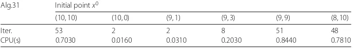
Table 2 Numerical results for Example 4.2
Alg.31 Initial pointx0
(10, 10) (10, 0) (9, 1) (9, 3) (9, 9) (8, 10)
Iter. 53 2 2 8 51 48
CPU(s) 0.7030 0.0160 0.0310 0.2030 0.8440 0.7810
The moving setK(x) =1≤i≤5Ki(x) where for eachx∈R5and eachi, the setKi(x) is
de-fined by
Ki(x) =
yi∈R|yi+
1≤j≤5,j=i
xj≥1
.
This problem was tested in [36] with initial pointx0= (1, 3, 1, 1, 2)T. They obtained the
appropriate solution after 21 iterates with the toleranceε= 10–3.
By the algorithm proposed in this paper, the numerical results obtained for this example are listed in Table 1 withc=γ = 0.5,ε= 10–3andX=K(x), and with different initial points.
Now, we consider a quasi-variational inequality problems and we solve it by using Al-gorithm 3.1 with the equilibrium functionf(x,y) =F(x),y–x.
Example4.2 Consider a two-person game whose QVI formulation involves the function
F= (F1,F2) and the multi-valued mappingK(x) =K1(x2)×K2(x1) for eachx= (x1,x2)∈R2,
where
F1(x) = 2x1+
8
3x2– 34, F2(x) = 2x2+ 5
4x1– 24.25,
and
K1(x2) ={y1∈R|0≤y1≤10,y1≤15 –x2},
K2(x1) ={y2∈R|0≤y2≤10,y2≤15 –x1}.
This problem was tested in [23]. The numerical results of Algorithm 3.1, abbreviated as Alg. 31, for this example are shown in Table 2 with different initial points.
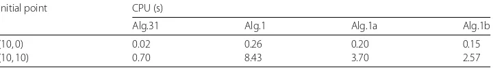
For this example, we chooseX=K(x) and takec=γ = 0.5. During the experiments, we set the stopping criterionε= 10–6. The numerical comparison of our proposed method
with the algorithms,i.e., Alg.1, Alg.1a, Alg.1b, proposed in [23] are given in Tables 3 and 4.
5 Conclusions
[image:13.595.117.480.183.233.2]Table 3 Iterations from Alg.31, Alg.1, Alg.1a and Alg.1b respectively
Initial point Number of iterations
Alg.31 Alg.1 Alg.1a Alg.1b
(10, 0) 2 3 2 2
[image:14.595.119.479.184.234.2](10, 10) 53 255 120 120
Table 4 The CPU time from Alg.31, Alg.1, Alg.1a and Alg.1b respectively
Initial point CPU (s)
Alg.31 Alg.1 Alg.1a Alg.1b
(10, 0) 0.02 0.26 0.20 0.15
(10, 10) 0.70 8.43 3.70 2.57
problem is established under pseudomonotonicity condition of the equilibrium function and the continuity of the underlying multi-valued mapping. Furthermore, we have shown that the generated sequence converges to the nearest point in the solution set to the initial point. The given numerical experiments show the efficiency of the proposed method.
Acknowledgements
This work was supported by the National Natural Science Foundation of China (Grant No. 11601261,11671228), and Natural Science Foundation of Shandong Province (Grant No. ZR2016AQ12), and China Postdoctoral Science Foundation (Grant No. 2017M622163).
Competing interests
The authors declare that they have no competing interests.
Authors’ contributions
All authors contributed equally to the writing of this paper. All authors read and approved the final manuscript.
Author details
1School of Management Science, Qufu Normal University, Rizhao Shandong, China.2Department of Applied
Mathematics, Southeast University, Nanjing, China.
Publisher’s Note
Springer Nature remains neutral with regard to jurisdictional claims in published maps and institutional affiliations.
Received: 7 November 2017 Accepted: 23 January 2018 References
1. Cho, S.Y.: Generalized mixed equilibrium and fixed point problems in a Banach space. J. Nonlinear Sci. Appl.9, 1083–1092 (2016)
2. Huang, N., Long, X., Zhao, C.: Well-posedness for vector quasi-equilibrium problems with applications. J. Ind. Manag. Optim.5(2), 341–349 (2009)
3. Li, J.: Constrained ordered equilibrium problems and applications. J. Nonlinear Var. Anal.1, 357–365 (2017) 4. Su, T.V.: A new optimality condition for weakly efficient solutions of convex vector equilibrium problems with
constraints. J. Nonlinear Funct. Anal.2017, Article ID 7 (2017)
5. Chen, H.: A new extra-gradient method for generalized variational inequality in Euclidean space. Fixed Point Theory Appl.2013, 139 (2013)
6. Chen, H., Wang, Y., Zhao, H.: Finite convergence of a projected proximal point algorithm for generalized variational inequalities. Oper. Res. Lett.40, 303–305 (2012)
7. Chen, H., Wang, Y., Wang, G.: Strong convergence of extra-gradient method for generalized variational inequalities in Hilbert space. J. Inequal. Appl.,2014, 223 (2014)
8. Qin, X., Yao, J.C.: Projection splitting algorithms for nonself operators. J. Nonlinear Convex Anal.18(5), 925–935 (2017) 9. Xiao, Y.B., Huang, N.J., Cho, Y.J.: A class of generalized evolution variational inequalities in Banach spaces. Appl. Math.
Lett.25(6), 914–920 (2012)
10. Chen, H.B., Qi, L.Q., Song, Y.S.: Column sufficient tensors and tensor complementarity problems. Front. Math. China (2018). https://doi.org/10.1007/s11464-018-0681-4
11. Chen, H.B., Wang, Y.J.: A family of higher-order convergent iterative methods for computing the Moore–Penrose inverse. Appl. Math. Comput.218, 4012–4016 (2011)
13. Wang, Y.J., Liu, W.Q., Cacceta, L., Zhou, G.L.: Parameter selection for nonnegativel1matrix/tensor sparse decomposition. Oper. Res. Lett.43, 423–426 (2015)
14. Wang, Y.J., Cacceta, L., Zhou, G.L.: Convergence analysis of a block improvement method for polynomial optimization over unit spheres. Numer. Linear Algebra Appl.22, 1059–1076 (2015)
15. Wang, C.W., Wang, Y.J.: A superlinearly convergent projection method for constrained systems of nonlinear equations. J. Glob. Optim.40, 283–296 (2009)
16. Chen, H.B., Chen, Y.N., Li, G.Y., Qi, L.Q.: A semidefinite program approach for computing the maximum eigenvalue of a class of structured tensors and its applications in hypergraphs and copositivity test. Numer. Linear Algebra Appl.
25(6), e2125 (2018)
17. Facchinei, F., Pang, J.-S.: Finite-Dimensional Variational Inequalities and Complementarity Problems. Springer, New York (2003)
18. Harker, P.T.: Generalized Nash games and quasi-variational inequalities. Eur. J. Oper. Res.54, 81–94 (1991)
19. Pang, J.-S., Fukushima, M.: Quasi-variational inequalities, generalized Nash equilibria, and multi-leaderfollower games. Comput. Manag. Sci.2, 21–56 (2005)
20. Zhang, J., Qu, B., Xiu, N.: Some projection-like methods for the generalized Nash equilibria. Comput. Optim. Appl.45, 89–109 (2010)
21. Nash, J.: Non-cooperative games. Ann. Math.54, 286–295 (1951)
22. Facchinei, F., Kanzow, C.: Generalized Nash equilibrium problems. Ann. Oper. Res.175, 177–211 (2010)
23. Strodiot, J.J., Nguyen, T.T.V., Nguyen, V.H.: A new class of hybrid extragradient algorithms for solving quasi-equilibrium problems. J. Glob. Optim.56, 373–397 (2013)
24. Blum, E., Oettli, W.: From optimization and variational inequality to equilibrium problems. Math. Stud.63, 127–149 (1994)
25. Pang, J.-S., Fukushima, M.: Quasi-variational inequalities, generalized Nash equilibria, and multi-leaderfollower games. Erratum. Comput. Manag. Sci.6, 373–375 (2009)
26. Pham, H.S., Le, A.T., Nguyen, B.M.: Approximate duality for vector quasi-equilibrium problems and applications. Nonlinear Anal., Theory Methods Appl.72(11), 3994–4004 (2010)
27. Taji, K.: On gap functions for quasi-variational inequalities. Abstr. Appl. Anal.2008, Article ID 531361 (2008) 28. Kubota, K., Fukushima, M.: Gap function approach to the generalized Nash equilibrium problem. J. Optim. Theory
Appl.144, 511–531 (2010)
29. He, B.S.: A class of projection and contraction methods for monotone variational inequalities. Appl. Math. Optim.
35(1), 69–76 (1997)
30. Iusem, A.N., Svaiter, B.F.: A variant of Korpelevich’s method for variational inequalities with a new search strategy. Optimization42, 309–321 (1997)
31. Han, D.R., Zhang, H.C., Qian, G., Xu, L.L.: An improved two-step method for solving generalized Nash equilibrium problems. Eur. J. Oper. Res.216(3), 613–623 (2012)
32. Wang, Y.J., Xiu, N.H., Zhang, J.Z.: Modified extragradient method for variational inequalities and verification of solution existence. J. Optim. Theory Appl.119, 167–183 (2003)
33. Zarantonello, E.H.: Projections on convex sets in Hilbert space and spectral theory. In: Contributions to Nonlinear Functional Analysis. Academic Press, New York (1971)
34. Konnov, I.V.: Combined Relaxation Methods for Variational Inequalities. Springer, Berlin (2001)
35. Rockafellar, R.T.: Monotone operators and the proximal point algorithm. SIAM J. Control Optim.14(5), 877–898 (1976) 36. Tran, D.Q., LeDung, M., Nguyen, V.H.: Extragradient algorithms extended to equilibrium problems. Optimization57,