Modeling And Simulation Of A Jet Dffusion Flame Of Hydrogen Solved By Applying The Rosenbrock Method

ORIGINAL RESEARCH ARTICLE

MODELING AND SIMULATION OF A JET DFFUSION FLAME OF HYDROGEN SOLVED BY APPLYING

THE ROSENBROCK METHOD

1

_{De Quadros, R.S.,}

_{Sehnem, R. and}

_{De Bortoli, A.L.}

1

_{UFPel, Graduate Program in Mathematical Modelling (PPGMMat), Pelotas, RS, Brazil}

2

_{UFRGS, Graduate Program in Applied Mathematics (PPGMAp) Bento Gon¸calves, 9500, 91509-900, Porto Alegre,}

RS, Brazil

ARTICLE INFO ABSTRACT

Problems involving chemical reactions have an important characteristic called stiffness, indicating that the solutions of the involved ODE systems vary in different orders of magnitude. So, it is needed to choose suitable numerical methods for obtaining numerical solutions that are stable and convergent at a low computational cost. The most used methods for dealing with this type of problem are the implicit methods, since they have a region of unlimited stability in the complex plane that allows large variations in step size. In this work we employ an L-stable method: the fourth-order Rosenbrock method of four stages. The reduced mechanism for the combustion of hydrogen is simulated and the results have good agreement with data found in the literature.

Copyright © 2019,De Quadros et al. This is an open access article distributed under the Creative Commons Attribution License, which permits unrestricted use, distribution, and reproduction in any medium, provided the original work is properly cited.

INTRODUCTION

Energy is an indispensable resource in everyone lives and combustion is the most used technology for conversion of it. For this reason, researchers have explored computational methods to develop practical combustion systems, specially as regards the reduction of the emission of pollutants into the atmosphere [1, 2]. The chemical kinetic modelling has become an important tool for interpreting and understanding the phenomena of combustion [3], leading to the development of several detailed and reduced reaction mechanisms to the combustion of different chemical compounds. Even today, fuels are predominantly derived from unsustainable mineral resources, petroleum and coal, whose combustion leads to environmental pollution, greenhouse gas emissions and problems with energy security [4]. But the high global demand of energy and the economic and environmental restrictions have leads to the pursuit for renewable sources of energy. Computer simulations with detailed kinetic mechanisms are complicated and, therefore, there is the need to develop, from these detailed mechanisms, the corresponding reduced mechanisms with fewer variables, maintaining a good level of accuracy and comprehensiveness for the desired applications [5].

*Corresponding author: De Quadros, R.S.,

UFPel, Graduate Program in Mathematical Modelling (PPGMMat), Pelotas, RS, Brazil

In this direction, based on the detailed mechanism given by Fisher et al. [6], available on the website of the Lawrence Livermore National Laboratory, the present paper develops a reduction strategy to obtain a two-step reduced kinetic mechanism for hydrogen. Reduced mechanisms for hydrogen combustion have been developed by many researches [7, 8, 9]. According to Peters and Rogg [7] the two-step mechanism is appropriate for hydrogen-air premixed and (non) diluted diffusion flames. There is an increasing interest in the study of hydrogen diffusion flames because of its key role in understanding hydrocarbon and biofuels combustion. Hydrogen can be obtained from fossil fuels or conveniently from renewable resources as a biofuel. The hydrogen is an important intermediate species in the oxidation of hydrocarbons and oxygenated fuels. The species H2, H, O, OH,

HO2 and H2O2 determine the composition of the radical pool in the majority of fuel reaction systems [10, 11]. Due to the existence of highly reactive radicals and fast reactions in the detailed mechanisms, the associate system of governing equations is stiff. One solution for this problem is the decrease of variables with the use of the assumptions of quasi-steady-state for species and partial equilibrium for reactions, whose purpose is to replace the differential equations by algebraic relations. This work is devoted to the study of a numerical method applied to H2−O2 chemical model, which is important

ISSN: 2230-9926

International Journal of Development Research

Vol. 09, Issue, 03, pp.26407-26413, March, 2019

Article History:

Received 24th _{December, 2018} Received in revised form 28th _{January, 2019}

Accepted 26th _{February, 2019} Published online 31st _{March, 2019}

Available online at http://www.journalijdr.com

Key Words: Stiffness, Rosenbrock, Combustion, hydrogen.

Citation: De Quadros, R.S., Sehnem, R. and De Bortoli, A.L. 2019. “Modeling and simulation of a jet dffusion flame of hydrogen solved by applying the rosenbrock method”, International Journal of Development Research, 09, (03), 26407-26413.

to evaluate the species concentration involved during the entire combustion process. The problems related to this process result in systems of ordinary differential equations (ODEs) with a special characteristic called stiffness, which occurs because the concentrations of the chemical species vary in different orders of magnitude. These are not the only problems with this type of characteristic, other examples appear in vibrations, electrical circuits and control theory. A system of equations is considered stiff when one or more variables change very quickly, while others change very slowly. This disparity over time is common in chemical systems in which reactions with radicals are very fast compared to reactions involving stable species. To solve stiff initial value problems, suitable numerical methods must be applied so that the numerical solution is stable and convergent at an acceptable computational cost. Although the treatment of stiff problems is quite frequent, there is not a mathematically precise definition that describes this characteristic well.

Curtiss and Hirschfelder [12], were the first to conclude that stiff problems need implicit methods because they have the region of adequate stability. More precisely, these methods have a region of unlimited stability that covers the entire complex half-plane with a negative real part or at least an unlimited part thereof. Later, Shampine and Gear [13] gave us a definition: the initial value problem for EDOs is stiff if the Jacobian matrix of the system has at least one eigenvalue, for which the real part is negative with high modulus, while the solution within most of the integration interval slowly changes. This definition is the one that best characterizes stiffness, explaining that these problems present solutions in which some components decay much faster than others. In this work, the fourth-order four-stage Rosenbrock method is employed. It is a simple step method, with development based on diagonally implicit Runge-Kutta (DIRK) methods. The method allows size variation of the integration step due to the unlimited stability region, so that it uses a small step size where the solution changes more quickly, and allows to increase step size in regions where the solution is softer, obtaining a reduction in computational costs. The method will be used in the solution for hydrogen combustion. The reaction mechanism of hydrogen oxidation is widely used in rocket propulsion and also becomes important as a subsystem in the oxidation of hydrocarbons, as seen in Turns [14]. Chamousis [15] shows some advantages and disadvantages of the use of hydrogen as a transportation fuel. As advantages, it can be mentioned: high energy yield (122kJ/g), produced from many primary energy sources, high diffusivity, water vapor as the major oxidation product, is the most abundant element and the most versatile fuel. As disadvantages, there are: low density, large storage areas, not found free in nature, low ignition energy (similar to gasoline) and is currently expensive. In this way, the study of this fuel and its behavior is fundamental for advances in the field of combustion of hydrocarbons and biofuels.

Flow equations and their discretization procedure: Favred filtering becomes convenient when writting the governing equations for turbulent flows. The set of equations for the combustion process includes the momentum (Navier-Stokes), enthalpy, species mass fraction and pressure. They are written as follow:

+ = − ̅+ , ……… (1)

+ = ̅ , ………. (2)

+ = ̅ , ………. (3)

where is the average density, the Favred averaged velocity, the Favred averaged mass fraction of species i, ithe reaction rate of

the species i, µ¯T the eddy viscosity, the Favred averaged

enthalpy.

The gradient of pressure can be obtained after solving a Poisson’s equation of the form [16]

∇ = ∆ ( )+ ( ) ……… (4)

The reaction rate of each species is given by

= / _{……… (5)}

In these equations, Re is the Reynolds, Pr the Prandtl, Scthe

Schmidt, Dathe Damk¨ohler and Zethe Zel’dovich numbers.

Temperature T˜ is obtained from enthalpy using a simple

Newton iteration

ℎ = ∑

ℎ

and density can be relaxed by

̅ =

with 0.1 < η < 0.8 to avoid numerical instabilities, since variations in density affect all other equations.

The set of equations was solved numerically. A central finite difference scheme was adopted for spatial derivatives of first and second orders. A nonuniform structured mesh was used in order to concentrate enough points at the exit of the injector and along the burner centerline.

( , , )=

( , , ) ( , , )

∆ ……… (8)

( , , )

= ( , , ) ( , , )

∆ ………. (9)

( , , )=

( , , ) ( , , ) ( , , )

∆ ……… (10)

and in similar manner in other directions. This set of equations can be summarized as:

∂y ∂t = f(y)

y(t ) = y

y = ( , , , ℎ) .

on the time-step size [18]. The eigenvalues of the Jacobian matrix for f characterize the stability of the system. Generally, a system is considered stiff when its eigenvalues are very different in magnitude [19].

Rosenbrock method

For the solution of the differential equations a L-stable method (to be defined soon) is implemented based on a class of Runge-Kutta methods known as Rosenbrock method. The conditions for L-stability require that the method be implicit. Implicit or semi-implicit Runge-Kutta methods are known to satisfy conditions for good stability [20]. In order to propose an alternative for the resolution of systems of implicit equations, usually solved by iterative processes, Rosenbrock [21] presented a new method. He developed a new class of single-step methods, which is based on linearizations of implicit Runge-Kutta methods. This avoids the resolution of non-linear systems to solve a sequence of linear systems, which facilitates the implementation of the method. This method is also named in the literature as a linearly implicit Runge-Kutta method or as diagonally implicit Runge-Kutta.

Consider a system of ordinary differential equations,

y′ = f (y), y(t0) = y0, ... (12)

(12)

Where in y = y(t) ∈ Rm, t ∈ R e f : Rm → Rm.

The coefficients used in the Rosenbrock method determine new stability properties and order conditions, different from the conditions of the Runge-Kutta methods. According to Lambert [22], to obtain a p-order Runge-Kutta method, we must expand the equation of Runge-Kutta s-stages in Taylor’s series to the desired order term and compare with the Taylor’s series of the corresponding exact solution. More details on the development of high-order Runge-Kutta methods are contained in Butcher [20] or Wanner et al. [23]. The concept of L-stability is very important, since A-stable methods that are not damped maximally when λh → −∞ do not generate satisfactory results [24]. This undesirable asymptotic behavior usually results in oscillatory solutions for very rigid systems. Thus, for extremely stiff systems it is desirable to develop L-stable rather than A-stable methods.

The four-stage fourth-order Rosenbrock method is given by:

= + ℎ (13 )

κ1=f(yn)/A(yn) (14a)

κ2=f(yn+ha21κ1)/A(yn) (14b)

κ3=f(yn+h(a31κ1+a32κ2))/A(yn) (14c)

κ4=f(yn+h(a41κ1+a42κ2+a43κ3))/A(yn) (14d)

(14d)

where ( ) = − ℎ ( ) .

The stability region of the method given by (13) with parameters from Table 1 and another four-stage A-stable fourth-order method developed by Bui [25], is shown in Figure 1.

The local error estimate, is:

=

with ρ the order of the method and the norm ∥ · ∥ is given by

∥y∥=

∅∑

∅

, (17)

where ϕ is the number of system variables.

Table 1. Parameters for the fourth-order Rosenbrock method with four stages

γ1 = 0, 9451564786 γ2 = 0, 341323172 γ3 = 0, 5655139575 γ4=−0,8519936081

a21 = −0, 500000000 a41 = −0,3922096763

a31=−0,1012236115 a42 = 0, 7151140251

a32=0,9762236115 a43=0,1430371625

Figure 1. Stability region of an A-stable and a L-stable four-stage fourth-order method, adapted from [25].

For a tolerance ε, the following procedure can be used to determine the time increase:

 If En+1> ε, the step is rejected and h should be reduced.  If, the step is accepted, but h should be reduced.

 If, the step is accepted and h is accepted.

 If, the step is accepted and h can be increased.

In this way, instead of using a small time-step across the whole integration interval to control regions with greater stiffness, we use an adaptive step control. Thus, in regions where the step should be reduced, it is done, whereas in regions with lower stiffness the step is increased in order to decrease the whole computational time to solve the system of equations. The variables yn∗+1 and yn+1 are calculated using time-steps h and h/2, respectively. To avoid divergence during the iterative process the increment for the step needs to be limited, which can be done by the following relation:

ℎ = ℎ 10, 0,1 ; ,

∆ …………. (18)

should be sufficiently small and, in the case

hn+1 the growth factor in the next iteration

to 1, instead of 10, as in equation (18).

Table 2. Hydrogen mechanism rate coe cients (units are mol, cm3, s, K and cal= mol).

Reaction A

1. OH + H2 = H + H2O 2.14E + 08

1b. H + H2O = OH + H2 5.09E + 09

2. O + OH = O2 + H 2.02E + 14

3. O + H2 = OH + H 5.06E + 04

4. H + O2+ M = HO2+ M 4.52E + 13

5. OH + HO2= H2O + O2 2.13E + 28

6. H + HO2 = OH + OH 1.50E + 14

7. H + HO2= H2+ O2 6.63E + 13

8. H + HO2 = O + H2O 3.01E + 13

9. O + HO2= O2+ OH 3.25E + 13

10. 2OH = O + H2O 3.57E + 04

11. H + H + M = H2 + M 1.00E + 18

12. H + OH + M = H2O + M 2.21E + 22

13. H + O + M = OH + M 4.71E + 18

14. O + O + M = O2+ M 1.89E + 13

15. HO2 + HO2 = H2O2 + O2 4.20E + 14

16. OH + OH + M = H2O2 + M 1.24E + 14

17. H2O2 + H = HO2 + H2 1.98E + 06

18. H2O2 + H = OH + H2O 3.07E + 13

19. H2O2 + O = OH + HO2 9.55E + 06

20. H2O2 + OH = H2O + HO2 2.40E + 00

Figure 2. First (left side) and third (right side) variables of Robertson model

Code verification

To check the implementation of the method used, a system of ordinary differential equations usually applied in numerical tests for stiff equations, called the Robertson model, was selected. The kinetic model of Robertson [26] is one of the

26410 De Quadros et al. Modeling and simulation of a jet dffusion flame of hydrogen solved by applying the rosenbrock method

case of rejection of iteration is made equal

cients (units are mol, cm3,

β EA

1.52 3449

1.30 18588

−0.40 0

2.67 6290

0.00 0

−4.83 3500

0.00 1000

0.00 2126

0.00 1721

0.00 0

2.40 −2112

−1.00 0

−2.00 0

−1.00 0

0.00 −1788

0.00 11982

−0.37 0

2.00 2435

0.00 4217

2.00 3970

4.04 −2162

e) variables of Robertson

the implementation of the method used, a system of ordinary differential equations usually applied in numerical equations, called the Robertson model, was The kinetic model of Robertson [26] is one of the

most known problems for the analysis of sti

model describes the kinetics of an autocatalytic reaction and the structure of the reactions is given by

y1→y2y2+y2→y2+y3

y

+

y

→

y

+

y

given by k1 = 0, 04, k2 = 3 · 107 are the chemical species involved.

Robertson has no defined units. The model can be described as:

= −0,04 + 10

= 0,04 − 10 − 3

= 3 × 10

The integration interval used was [10 conditions

y1(t0) =1,

y2(t0) =0,

y3(t0) =0.

The points obtained by the integration of the Rosenbrock method are compared

[27], which used the Modified Extended Backward Differentiation Method (MEBDF), and with the work of Nagy [28], in which a package

developed (called Reaction Kinetics) and compared with a MATLAB internal command.The results shown in

are in good agreement with those observed in the literature.

Solution of a Hydrogen Turbulent

simplify the chemical kinetics involved of the problem, a reduced mechanism hypotheses, such as steady-state steady-state hypothesis is valid produced by slow reactions and their concentrations remain small equilibrium is justified when the backward reactions are much velocities of the mechanism [29].

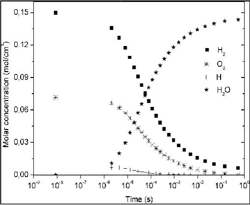
Figure 3. Molar concentrations obtained by integration of the reduced mechanism for

De Quadros et al. Modeling and simulation of a jet dffusion flame of hydrogen solved by applying the rosenbrock method

most known problems for the analysis of stiff methods. The model describes the kinetics of an autocatalytic reaction and the structure of the reactions is given by

(19)

and k3 are the specific velocities

7

and k3 = 104 and y1, y2 and y3

involved. The model proposed by Robertson has no defined units. The model can be described as:

,

× 10 , (20)

The integration interval used was [10−3, 105] with initial

(21)

the integration of the model with the compared next with the work of Silva Modified Extended Backward erentiation Method (MEBDF), and with the work of Nagy package for Mathematica software is on Kinetics) and compared with a command.The results shown in Figure 2 are in good agreement with those observed in the literature.

Turbulent jet Diffusion Flame: To involved and favor the resolution mechanism is made using some state and partial equilibrium. The for intermediate species that are and consumed by fast reactions, so small [14]. The hypothesis of partial the velocities of the forward and much greater than the other specific

[29].

Molar concentrations obtained by integration of the

reduced mechanism for H2 combustion

Table 3. Comparison between the equilibrium mole fractions

Species Present work

H2 0.0149

O2 2.11E – 9 H 3.74E – 9

H2O 0.3470

N2 0.638

Figure 4. Sketch of a jet flame

Mechanisms of hydrogen combustion: Consider the reactions

1-20 presented by Marinov [30], according to Table 2. After applying the hypothesis of partial equilibrium for those reactions with high specific forward and backwar

it remains the reactions 1, 3, 11, 12, 13 and 14. Considering the steady-state assumption for the species

following two-step mechanism among four species for hydrogen

I3H2+O2=2H+2H2O

IIH + H + M = H2 +M

where M is an inert needed to remove the bond energy that is liberated during recombination [29].

The system of ordinary differential equations resulting from these reactions is

d[H2]/dt=−3ωI′+ωI I′,

d[H]/dt=2ωI′−2ωI I′,

d[O2]/dt=−ωI′,

d[H2O]/dt=2ωI′.

NUMERICAL RESULTS

To obtain the behavior of the species concentration in relation to time, the system of reactive equations was

fourth order Rosenbrock method with four

26411 International Journal of Development Research,

the equilibrium mole fractions

Gaseq 0.015 0.006 no info

0.324 0.646

Sketch of a jet flame

Consider the reactions 20 presented by Marinov [30], according to Table 2. After applying the hypothesis of partial equilibrium for those reactions with high specific forward and backward velocities, it remains the reactions 1, 3, 11, 12, 13 and 14. Considering state assumption for the species OH, it results the step mechanism among four species for

(22)

is an inert needed to remove the bond energy that is

erential equations resulting from

(23)

obtain the behavior of the species concentration in relation was solved by the stages defined by

the equation 13 and using the

in the table 1. The tolerance for the error used was The simulations were done assuming a temperature of 800 In Figure 3 the species molar concentrations in relation to time are shown. In the Table 3 a comparison

generated through the Gaseq program ( co.uk/), which provides the molar

the equilibrium is obtained. Gaseq uses a method based on the minimisation of free energy (NASA method).

Figure 5. Mass fraction of H2

centerline

Figure 6. Mass fraction of H2

and 60

International Journal of Development Research, Vol. 09, Issue, 03, pp.26407-26413, March

the parameters of Bui [31] shown tolerance for the error used was ϵ = 10−7. The simulations were done assuming a temperature of 800K. In Figure 3 the species molar concentrations in relation to time comparison is made with the data Gaseq program (http://www.gaseq. molar fraction of the species when equilibrium is obtained. Gaseq uses a method based on the minimisation of free energy (NASA method).

2, O2 and H2O along the burner

centerline

2 and H2O at positions X/R=40

and 60

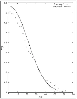
Figure 7. Temperature T profile at position X/R=40

We suppose air as a mixture composed of 23

76.28% of N2. The results are consistent with those provided by Gaseq, but while Gaseq only report the concentration at equilibrium, our data provide information on the whole process. Following, we present the results for a turbulent jet diffusion flame as shown in Fig. 4. Numerical

flame are indicated as”num” in the figures.

chosen because it represents the class of nonpremixed One employs a duct of cylindrical cross section

De= 0.3 and the fuel is injected from a tube of

0.07. The duct length corresponds to 10 De

used to compare the results (www.ca.sandia.gov/TNF).Since the flame is governed by hydrodynamics,

decreasing of the mixture fraction along the burner centerline. The mass fraction of fuel H2, oxidizer O2 and product

shown in Fig. 5. The radial mass fraction distribution, shown in Fig. 6, can be reasonably approximated by a Gaussian function. The temperature profile, presented

reasonable agreement with the experiment. It rises rapidly in the rich part of the flame and decreases by

lean flame region.

Conclusions

In this work the four-stage fourth-order Rosenbrock employed for solving a turbulent jet di

hydrogen. It is applied in the EDOs system resulting from the modeling of chemical kinetics for hydrogen combustion. Also is presented a reduced mechanism for hydrogen with two reactions and four species, which represents well the behavior of the complete system containing 21 reactions and eight species. It is believed that the great impact of this w

the qualitative and quantitative model for the

research involving stiffness equations, especially in the field of combustion, since the numerical simulation of mechanisms

26412 De Quadros et al. Modeling and simulation of a jet dffusion flame of hydrogen solved by applying the rosenbrock method

profile at position X/R=40

suppose air as a mixture composed of 23.7% of O2 and The results are consistent with those provided by Gaseq, but while Gaseq only report the concentration at information on the whole present the results for a turbulent jet Numerical results of the jet The jet flame was nonpremixed flames. section with diameter fuel is injected from a tube of diameter D =

e. The H2 flame is

(www.ca.sandia.gov/TNF).Since hydrodynamics, occurs an axial of the mixture fraction along the burner centerline. and product H2O are distribution, shown in Fig. 6, can be reasonably approximated by a Gaussian in Fig. 7, shows a . It rises rapidly in by expansion in the

Rosenbrock method is for solving a turbulent jet diffusion flame of It is applied in the EDOs system resulting from the hydrogen combustion. Also is presented a reduced mechanism for hydrogen with two reactions and four species, which represents well the behavior of the complete system containing 21 reactions and eight It is believed that the great impact of this work is on the development of equations, especially in the field of combustion, since the numerical simulation of mechanisms

that represent this phenomenon, can become di involves highly reactive radicals, which brings sti system. In this way, the simplifications contribute to the achievement

stiffness of the system. Furthermore, the numerical method presented here contains features that allow reduction in computational cost and stability

in the temporal step, which may

researches. For future works, it is suggested to apply the same procedure for a larger biofuel molecules, such as methanol, ethanol and biodiesel.

Acknowledgments: This research Federal University of Pelotas,

University of Rio Grande do Sul. R. Sehnem thanks the financial support from CAPES,

Improvement of Higher Education Personnel. Prof. De Bortoli gratefully acknowledges the financial support of CNPq, under process 303816/2015-5.

REFERENCES

Aiken, R. C. Stiff Computation, Oxford University Press, Incorporated, 1985.

Andreis, G. A. De Bortoli, 2014. difusivas, Novas Edi¸c˜oes GmbH Co. KG Saarbroken

Bui, T. Some a-stable and l-stable methods for the numerical integration of stiff ordinary

of the ACM 3 (1979) 483– Bui, T. On an l-stable method for sti

Inf. Proc. Letters 6 (1977) 158 Bui, T. T.R. Bui, Numerical methods

of ordinary differential equations, Modelling 5 (1979) 355–358.

Butcher, J. Implicit Runge-Kutta processes, Mathematics of Computation 85 (1964) 50–

Chamousis, R. Hydrogen: Fuel Research Society.

Curtiss, C. J. Hirschfelder, Integration of sti Proceedings of the National

(1952) 235–243.

Demirbas, A. 2009. Biofuels securing the planets future energy needs, Energy Conversion and Managemen 50

2249.

Fisher, E. W. Pitz, H. Curran, C. Westbrook,

chemical kinetic mechanism for combustion of oxygenated fuels, Proceedings of the Com

1579–1586.

Griffiths, J. 1995. Reduced kinetic

to practical combustion systems, Progress in Energy and Combustion Science 21 (1995) 25

Hairer, E. S. Norsett, G. Wanner,

equations I: Nonstiff problems, Springer, New Lambert, J. Numerical Methods for Ordinary Di

Equations: The Initial Value Sons, New York, 1991.

Li, I. Z. Zhao, K. Kazakov, F. Dryer, An updated comprehensive kinetic model of hydrogen combustion, International Journal of Chemical Kinetics 36 (2004) 575.

Marinov, N. A detailed chemical temperature ethanol oxidation, Chemical Kinetics 31 (1999)

De Quadros et al. Modeling and simulation of a jet dffusion flame of hydrogen solved by applying the rosenbrock method

that represent this phenomenon, can become difficult since it highly reactive radicals, which brings stiffness to the the simplifications used in this paper achievement of good results, with reduced ness of the system. Furthermore, the numerical method contains features that allow reduction in computational cost and stability that allows a great variation may represent an advance in other future works, it is suggested to apply the same ofuel molecules, such as methanol,

research is being developed at UFPel, Pelotas, and at UFRGS, Federal University of Rio Grande do Sul. R. Sehnem thanks the financial support from CAPES, Coordination for the Improvement of Higher Education Personnel. Prof. De Bortoli gratefully acknowledges the financial support of CNPq, under

Computation, Oxford University Press,

2014. Solu¸c˜ao via LES de chamas oes Acadˆemicas: Omniscriptum

en.

stable methods for the numerical ordinary differential equations, Journal

–493.

stable method for stiff differential equations, 158–161.

methods for extremely stiff systems equations, Applied Mathematical 358.

Kutta processes, Mathematics of –64.

Fuel of the future, The Scientific

Curtiss, C. J. Hirschfelder, Integration of stiff equations, National Academy of Sciences 3

Biofuels securing the planets future energy needs, Energy Conversion and Managemen 50, 2239–

Fisher, E. W. Pitz, H. Curran, C. Westbrook, 2000. Detailed hemical kinetic mechanism for combustion of oxygenated fuels, Proceedings of the Com- bustion Institute 28 (2)

kinetic models and their application combustion systems, Progress in Energy and Science 21 (1995) 25–107.

Wanner, Solving ordinary differential problems, Springer, New York, 1987. Lambert, J. Numerical Methods for Ordinary Differential

Value Problem, John Wiley and

Li, I. Z. Zhao, K. Kazakov, F. Dryer, An updated comprehensive kinetic model of hydrogen combustion, International Journal of Chemical Kinetics 36 (2004) 566–

chemical kinetic model for high ethanol oxidation, International Journal of

Nagy, A. J. T´oth, D. Papp, Reaction Kinetics: Exercises, Programs and Theorems, Mathematical and Computational Chemistry, Springer, New York, 2014.

Nikolaou, Z.M. J.Y. Chen, N. Swaminathan, A 5-step reduced mechanism for combustion of co/h2/h2o/ch4/co2 mixtures with low hydrogen/methane and high h2o content, Combust. Flame 160 (2013) 56–75.

Pepiot-Desjardins, P. H. Pitsch, 2008. An automatic chemical lumping method for the reduction of large chemical kinetic mechanisms, Combustion Theory and Modelling 12 (6) 1089–1108.

Pereira, F. N. G. Andreis, A. D. Bortoli, N. Marcílio, Analytical-numerical solution for turbulent jet diffusion flames of hydrogen, Journal of Mathe- matical Chemistry

51 (2013) 556–568.

Peters, N. Turbulent Combustion, Cambridge University Press, 2000.

Peters, N. Rogg, B. 1993. Reduced kinetic mechanisms for applications in combustion systems, Springer, Berlin. Pitsch, H. H. Steiner, Large-eddy simulation of a turbulent

piloted methane/air diffusion flame (sandia flame d), Physics of Fluids 12(10) (2000) 2541–2554.

Robertson, H. The solution of a set of reaction rate equations, Numerical analysis: an introduction (1966) 178–182.

Rosenbrock, H. Some general implicit processes for the numerical solution of differential equations, The Computer Journal 5 (1963) 329–330.

Saxena, P. 2006. A. Williams, Testing a small detailed chemical-kinetic mechanism for the combustion of hydrogen and carbon monoxide, Combustion and Flame 145, 316–323.

Shampine, L. C. Gear, A users view of solving stiff ordinary differential equations, SIAM review 1 (1979) 1–17. Shieh, D.-S. Y. Chang, G. Carmichael, The evaluation of

numerical techniques for solution of stiff ordinary differential equations arising from chemical kinetic problems, Environmental Software 3 (1) (1998) 28–38.

Silva, D. Aprimoramento de m´etodos num´ericos para a integra¸c˜ao num´erica de sistemas alg´ebrico-diferenciais, Master’s thesis, COPPE/UFRJ, Rio de Janeiro (2013). Strohle, J. T. Myhrvold, Reduction of a detailed reaction

mechanism for hydrogen combustion under gas turbine conditions, Combustion and Flame 144 (2006) 545–557. Turns, S. An introduction to combustion, McGraw Hill,

Boston, 2000.

Vaz, F. A. D. Bortoli, 2014. A new reduced kinetic mechanism for turbulent jet diffusion flames of bioethanol, Applied Mathematics and Computation 247., 918–929.

*******