5907
LARGE SCALE SENSOR DATA PROCESSING BASED ON
DEEP STACKED AUTOENCODER NETWORK
1NAGWA ELARABY, 2MOHAMMED ELMOGY, 3SHERIF BARAKAT
1,3Information System Department, Faculty of Computers and Information, Mansoura University, Egypt
2Information Technology Department, Faculty of Computers and Information, Mansoura University, Egypt
E-mail: 1[email protected], 2[email protected], 3[email protected]
ABSTRACT
Recently, Internet of Things (IoT) extremely populated by massive amounts of connected embedded devices, which are gathering large volumes of real-time heterogeneous data. Hence, IoT becomes an archetypal instance of Big Data. The collected IoT Big Data may not be profitable unless we evaluate and accurately exploit them. Providing mining for large scales of raw sensor data is an open challenge. To cope with this challenge, we proposed a system that operates in two modes, which are preparation and processing. The preparation mode converges on reducing the factors that hinder making efficient processing by focusing on three stages. First, handling missing data by applying interval-valued fuzzy-rough feature selection methodology. It highlights the most important features that contain missing data and gets rid of the others. Then, Maximum Likelihood (ML) approach is used for estimating the missing values. Second, anomalies are detected by initially utilizing K-nearest neighbors (KNN) algorithm then removing the detected ones from the data. Third, the dimensionality of nonlinearly separable data is reduced by exploiting Self-Organizing Map (SOM) network. In the processing mode, we passed the prepared data to a straightforward classifier based on a Deep Learning (DL) approach. We used autoencoder networks in constructing a deep network, which is the Deep Stacked Autoencoder (DSAE). The extracted features by the DSAE are non-handcrafted and task dependent, which gives it the most discriminative power to work as an efficient classifier. We apply the proposed model to PAMAP2 Physical Activity Monitoring data set. The results show that DSAE achieves high accuracy (99.8%) compared to the state-of-the-art classifiers.
Key words:Internet of Things (IoT), Big Data, Deep Learning (DL), Deep Stacked Autoencoder (DSAE).
1. INTRODUCTION
Our environment is surrounded by sensors, which continuously gather large volumes of real-time heterogeneous data about our living life [1]. Day after day, smartphones, cameras, cars, and smart homes capture countless useful data for solving several problems, such as healthcare, targeted advertising, traffic flow, and fraud detection. As a result, zettabytes of sensed data are generated. Hence, the Internet of Things (IoT) becomes an archetypal instance of Big Data. It is predicted that more than 26 billion of things will be connected to the Internet in 2020. The collected IoT Big Data may not be profitable unless we evaluate, construe, recognize, and accurately exploit them. Providing trustworthy mining for large scales of raw sensor data remains an open challenge [2].
On the other hand, the world becomes dynamic and complex. Under such conditions, machine learning and signal processing techniques regularly confused and appointed to sensor inference [2]. Machine learning helps in
getting millions of machines together to recognize what is the purpose of the data prepared by human beings [3]. In IoT community, machine learning can aid in controlling massive amounts of heterogeneous data made by those machines by enabling an extensive range of classification, regression, and density estimation tasks. Recently, the most promising machine learning approaches for dealing with IoT is Deep Learning (DL) [4]. The consideration of DL for these systems is now in progress with promising early results [2].
5908 structure of deep architectures. By this way, the nonlinear transformations learn and construct more abstract representations from less abstract ones. The final data representation that achieved by deep architectures is a highly nonlinear function of the input data, which can be treated as features in building classifiers.
More obviously, suppose there is some animal images are applied to a DL algorithm. The successive hidden layers will learn all features of the input images as follows. Firstly, the edges of images in different orientations is learned by the first layer. Secondly, the learned edges are passed to the second layer to enable it to extract more other complicated features, such as object eyes and noses. Thirdly, the third layer composes all these features to learn features of shapes of different
objects. Finally, the final high-level
representations of the input can be used in the application of object recognition. It is clear that how a DL algorithm catches complicated and more abstract data representations depending on a hierarchical architecture.
Tapping the knowledge that is extracted and made accessible by DL algorithms in the perspective of Big Data analytics is a novel study [7, 8]. DL capabilities in dealing with massive volumes of unlabeled data, learning aspects of data variation, and working in online mode for instantly coming of data streams make it a dynamic and effective tool for solving Big Data analytics problems. Deep Convolutional Neural Networks (DCNNs), Deep Belief Networks (DBNs), and Deep Convex Networks (DCN) are well-known DL models [9]. Recently, these models have been applied with unprecedented success in essential tasks of Big Data analytics, such as dimensionality reduction, natural language processing, motion modeling, object detection, speech recognition, and information retrieval.
The objective of this paper is to provide a solution for dealing with the scale of Big Data in IoT. It provides prediction model for IoT Big Data that faces several key challenges, such as the abundant existence of missing values, presence of a high range of anomalies, high variety of data types, and massive volumes of data instances. We handled each challenge independently. For the existence of missing values, we applied interval-valued fuzzy-rough feature selection methodology to highlight the most important features that contain missing data and getting rid of the others. Then, we use Maximum Likelihood (ML) approach for replacing the missing values. For the presence of anomalies, we initially utilized
K-Nearest Neighbor (KNN) algorithm to detect the unusual patterns that do not belong to frequent events then we removed all these patterns from the data. For the nonlinear separability of data, we exploited Self-Organizing Map (SOM) to obtain low-dimensional views of data. After that, we proposed Deep Stacked Autoencoder (DSAE) network as a DL-based classifier to efficiently analyzing such volumes of data. The key attribute of DSAE is accompanying different processing units that yield to provide an effective representation of native occurrence of sensor signals in various scales. The extracted features by the DSAE are non-handcrafted and task dependent which gives it the most discriminative power to work as an efficient DL classifier for representing a high-level abstraction of IoT data.
The remainder of this paper is organized as follows. Section 2 presents some existing studies in providing reliable and efficient classification model for recognizing IoT Big Data. Section 3 illustrates the preparation and processing modes of the proposed system. Section 4 discusses the experimental results and discussion. Finally, Section 5 presents the conclusion and future work.
2. RELATED WORK
In this section, we introduce a brief overview for some of the current studies that are related to providing reliable and efficient classification model for recognizing IoT Big Data. For example, Paniagua et al. [10] intended to abstract valuable information about human activities from massive volumes of raw sensor data obtained by an accelerometer. They utilized the ability of MapReduce operations in expanding the scope of the initial data set that helps in empowering the precision of training frameworks and scaling to sensible execution times. They employed MapReduce on the cloud as a parallel computing procedure for training and classifying the activities. The obtained sensor data are emptied on the cloud and processed based on Iterative Dichotomizer 3, Naive Bayes, and KNN classifiers. The performance analysis showed that the recognition of activities was more feasible with those algorithms. However, MapReduce on the cloud is still a high-cost procedure.
5909 vectors at once with the use of recent multi-core GPUs then the final representation was obtained by merging the chunks results together. GM-SOM intelligently achieved more accurate classification by concentrating on the selection of potential centroids of data clusters. Then, it produced them as the weight vectors in the final calculations. GM-SOM was used to process HAR data set [12] that represented different human activities recorded by smartphone sensors. Results showed that the proposed modification to the standard SOM performs well. This model success in recognizing similarities of data due to the nonlinearity of classes separation.
Dai and Ji [13] found that the traditional algorithms of sequential decision trees become not suitable for processing large volumes of real time data. So, they proposed a distributed employment of original C4.5 algorithm on MapReduce and installed it on a Hadoop cluster. The implementation of the proposed model followed four repetitive steps. First, data preprocessing to prepare data for MapReduce processing. Second, selection to select best attributes. Third, upgrade to update both hash and count tables. Finally, a tree growing by constructing a connection between nodes. Extensive experiments were conducted on a massive synthetic data set. The results indicated that the implementation of the C4.5 algorithm on MapReduce presented efficiency regarding time and scalability. However, other efficient algorithms may achieve higher accuracy than C4.5, such as Case-based Reasoning (CBR) algorithm [16].
Coninck et al. [14] introduced a new architecture of Artificial Neural Networks
(ANN) with the objective to obtain
contextualized and actionable information from enormous volumes of data coming from IoT. The proposed architecture was the Big-Little Neural Network (BLNN). The idea of BLNN was to use two networks in the classification process, which is a big remote neural network (NN) executed on the cloud and a little NN executed on the embedded devices. The little NN was used only to classify high priority classes with limited CPU power locally. Then, the big NN classifies remain classes remotely with more computational power. The BLNN architecture was evaluated using large scale data set. Experimental results showed that the BLNN achieved fast response time with high classification accuracy compared to the natural NNs. On the other hand, working on the
cloud allows better classification but needs more bandwidths.
Shilton et al. [15] proposed a Dynamic Planar One-class Support Vector Machine (DP1SVM) model to face the challenge of dealing with streaming data, which is collected from large-scale networks. DP1SVM is a modified usage of the incremental binary SVM. DP1SVM followed two steps for incrementally learning new data. The first step was the automatic remoteness for historical data from the system. The second step was updating the model parameters to fit the new state without the need to retraining the machine from scratch. Two IoT data sets were used to evaluate the model. Results proved its practical ability to learn streaming data with lower computational overhead and adequate execution time. However, this work did not take the heterogeneity of data in its consideration.
Chettri et al. [16] utilized several data computation algorithms for recognizing massive amounts of unknown data collected from IoT. Three supervised learning classifiers are introduced, which are KNN, Naive Bayes, and CBR. Among the presented algorithms, they proved that CBR classifier was the most suitable classifier for the proposed system. CRB in comparison to the other algorithms had many advantages. It could work with massive amounts of data, deal with the complex as well as incomplete cases, and rapidly provide solutions to problems with high accuracy. However, no data sets were used in this work to evaluate the proposed algorithm.
5910 Mo et al. [18] designed a DL model based on CNN and multilayer perceptron to diagnose large scale physical sensory data. The developed model consisted of seven layers, which were six hidden layers and multilayer perceptron layer. The hidden layers were three convolutional layers and three max-pooling layers, which are used for feature extraction. The multilayer perceptron layer was used to arrange the extracted features to their predicted classes. For optimization purpose, the model followed two stages: preparation and regularization. The preparation stage concluded normalizing the input data, initializing the value of parameters, and disorderly the training sequence of the sample. The regularization stage included preventing overfitting by adjusting the system parameters as small as possible and using a Max-norm algorithm to do not allow the weight to become very large. Experimental results of the proposed model showed its efficiency regarding time and accuracy. However, the multilayer perceptron is an old procedure and can be replaced with the Recurrent Neural Network.
Ordóñez and Roggen [19] aimed to automate feature learning and modeling massive inputs of raw sensor data by suggesting a DL-based model. The proposed model was DeepConvLSTM, which composed of convolutional and long short term memory recurrent layers. The convolutional layers worked as a feature extractor to extract valuable representations from the sensor input data in feature maps. Then, the temporal dynamics of the activation of the feature maps were modeled by the recurrent layers. The DeepConvLSTM framework was evaluated on two human activity recognition data sets. Results
showed that the proposed framework
outperformed the published state-of-the-art results. Also, it showed the ability of the DeepConvLSTM in working on the raw sensor data directly with only insignificant pre-processing, which made it mostly general. However, this framework is not scalable for highly corrupted raw sensor data sets.
Alsheikh et al. [20] focused on building up a framework that empowers time-effective Mobile Big Data (MBD) analytics by using DL models with an abundance of modeling parameters. Apache Spark was used to speed up the analysis process of MBD by parallelizing the learning of deep models over a high-performance computing cluster. The overall MBD was sliced into many partitions, and a spark worker learned the deep partial model of each partition. Then, a deep master model was constructed by averaging the
parameters of all partial models. A mobile data with millions of samples was used to evaluate the framework. The results showed that deep models were outstanding the current convolutional learning models. However, there is a need for more work in crowd labeling methods for MBD.
In summary, a large number of computation algorithms have been developed for recognizing enormous volumes of unknown data collected from IoT. They encompassed several techniques in different disciplines. However, it is hard to say that one method is obviously superior to other methods. The limitations of the previously mentioned literature can be concluded in the following points. First, the concentration was in introducing data processing frameworks, and not on preprocessing framework. Second, training shallow architectures achieved limited flexibility and scalability. Third, working on the cloud needs high cost and more bandwidth. Finally, all introduced DL-based methods are generative architectures, which have limited power in avoiding misspecification.
To overcome the limitations above, we intend to utilize DL in building a classification system for dealing with IoT Big Data, but with using different DL architecture. We construct the proposed model by using stacked autoencoders instead of stacked Restricted Boltzmann Machines. The hierarchal structure and discriminative power of stacked autoencoders help in making efficient feature learning and extraction. Then, we add a softmax layer to the stacked autoencoders to classify the extracted features to their predicted classes. In addition, we prepared the IoT Big Data before passing it to the proposed model to guarantee more accurate classification results.
3. THE PROPOSED SYSTEM
IoT is extremely occupied by massive numbers of heterogeneous connected sensors. The connected sensors usually generate a large volume of real-time data sets, which have various and composite structure. Big data processing is not an easy task and fetches exclusive challenges. To cope with this challenge, we proposed a system that can work as a key enabler for IoT Big Data. The proposed system operates in two modes: preparation and processing, as shown in Fig. 1. The preparation mode converges on reducing the factors that hinder making efficient processing by focusing on three main stages. First, handling the existence of missing data by applying
5911 methodology. It highlights the most important features that contain missing data and gets rid of the others. Then, ML approach is used for estimating the missing values. Second, anomalies are detected by initially utilizing KNN algorithm then removing the detected ones from the data. Third, the dimensionality of nonlinearly separable data is reduced by exploiting SOM network. The processing mode enables passing the prepared data to a straightforward classification model based on a DL approach. We make use of autoencoder networks in constructing a deep network. The proposed DSAE consists of a stack of autoencoders accompanying with a softmax layer. The extracted features by the DSAE are non-handcrafted and task dependent, which gives it the most discriminative power to work as an efficient DL classifier for representing a high-level abstraction of IoT Big Data. Finally, we evaluate the performance of our proposed classifier regarding accuracy, specificity, and sensitivity. The main stages of the proposed framework are discussed in the sequent subsections.
3.1. The Preparation Mode
The collected sensor data are loosely controlled. They often have missing and out-of-range values, impossible data combinations, high-dimensional, and nonlinearly separable data. These characteristics lead to the existence of low-quality data. Because of the low-quality of data affects data processing results. We need to make efficient preparation for improving the quality of collected raw sensor data. In our proposed system, we consider three sequential steps for raw sensor data preparation, which are handling the existence of missing data, detecting anomalies, and reducing the dimensionality of nonlinearly separable data.
3.1.1. Handling missing data
Sensors are not only collecting data about the surrounding physical phenomena but also transmitting these data to servers and other nodes
through a wireless network. The sensor transmitted data may be corrupted or missed owing
to many causes, such as unfavorable
environmental circumstances that make unstable communication links between sensor nodes, limited battery power at the sensor nodes or high bit error rates and packet loss in transmitting data streams. The sensor processing data with the existence of missing stream values will lead to insufficient results with less accuracy. To solve this problem, the missing data must be estimated as precisely as possible. As shown in Fig. 2, we recommend making reduction before estimating missing values. We noticed that not all the features that contain missing data are necessary. There may be redundant and not crucial features that will not retrieve any profit in assigning their missing values. So, making the estimation process limited to the most important features will rise proficiency and reduce the needed time for handling missing data. We applied interval-valued fuzzy-rough feature selection methodology to handle missing data [21, 22]. This methodology is more natural as it combines the concepts of vagueness that are introduced in fuzzy sets and concepts of coarseness introduced in rough sets. So, it presents a better way for controlling uncertainty in real data types that make it an available tool for making reduction effectively.
The basic idea of interval-valued fuzzy-rough feature selection methodology is to partition the features into three rough sets: insignificant, significant, and intermediate features. Then, the membership of each feature to the defined sets is calculated by using fuzzy membership function using equations (1) and (2) to reserve ranks of roughness in boundary region [19]. Only features that belong to significant rough set are remained and other features are removed.
μ x inf ∈ μ x, y , μ y (1)
5912
5913 Figure 2: The block diagram of handling missing
data.
where μ , μ are the interval-valued fuzzy
rough sets, μ x, y is the interval-valued fuzzy
tolerance relation, is a fuzzy implicator, is a
fuzzy t-norm, R is the fuzzy similarity relation
induced by the subset of features P, is a fuzzy
set, and x, y ∈ .
After reduction, handling the missing data can be done by using one of four approaches, which are a deletion, ML, imputation or machine learning procedures that able to handle missing data without an explicit imputation [23]. On the other hand, other researchers argued that there is no guaranteed approach for all missing data types [24]. We suggest applying ML approach because it is the most appropriate for replacing missing in sensor readings. This approach models the input data distribution by the Expectation Maximization (EM) algorithm to assume the value of unknown readings. It is based on several iterations of two steps [25]. First, expectation step substitutes the missing parameters with conditional expectations that are observed from the distribution by using equation (3). Maximization step to fill in the missing data with the maximum likelihood estimates of the parameters by using equation (4). So, this approach can replace the missing readings with the most appropriate values that will adjust the corruption and losing in sensor data.
q x p x|z; θ (3)
θ arg max q x log x, z; θ dx (4)
where x is the unobserved variables, z is the
observed variables, and θ is the probabilistic
parameters.
3.1.2. Detecting anomalies
Anomalies are usually referred to the existence of unusual measures or patterns that do not belong to ordinary events. Consequently, such measures will cause noise in data and present slanted distributions, which may make difficulty in fitting accurate computational models of the data. Anomalies are often spread abundantly in large data sets [26]. Therefore, detecting anomalies is a way to decrease the danger of concluding weak results based on wrong data and aid in avoiding and fixing the effects of faulty behavior.
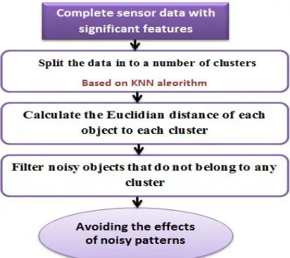
Figure 3: The block diagram of detecting anomalies.
As shown in Fig. 3, we recommend KNN algorithm for Anomaly detection. KNN has confirmed to be very effective in detecting anomalous behaviors in large-scale data streams [26]. It can detect outliers in both discrete and continuous attributes in large data sets by following two phases. Firstly, the received data set is split into a number of clusters .Secondly, the
Kth nearest neighborhood for each object in each
cluster is calculated using the Euclidian distance, see equation (5). Therefore, noisy objects that do not belong to any cluster will be highlighted [27]. So, KNN takes into consideration each instance to give an accurate detection for noisy ones.
5914
where x and y are k-dimensional vectors,
indicated by x x ,x , … , x and y
y ,y , … , y .
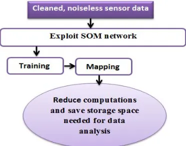
3.1.3. Dimensionality reduction
Sensors are usually collect streams of heterogeneous and nonlinearly separable data. For example, temperature sensor readings will be varied from the motion sensor readings, camera pickups, and so on. The precision and cumulative ubiquity in the collected data from different sensor types become a challenge. Analyzing this data will entail high computations and more memory capacity. Therefore, reducing the dimensionality of nonlinearly separable data will be a favorable implement to form a low-dimensional component space for the raw sensor data. Low-dimensional spaces will handle the
complexity of data analysis regarding
computations and storage space.
Principal component analysis (PCA) is the standard dimensionality reduction method, which provides a low-dimensional demonstration of data that are presumed to fall in subspace.
However, PCA gives an ineffective
representation with useless dimensions if the data resides in a nonlinear structure. So, as shown in Fig. 4, we recommend using SOM in getting rid of the high dimensionality of sensor data. SOM operates as a feedforward unsupervised NN, which reserves the topological characteristics of the input space by using a neighborhood function based on equation (6) [28]. This makes SOM able to perform the efficient mapping from high-dimensional to low-high-dimensional data. SOM reduces the dimensionality of nonlinearly separable data without conceding integrity compared to PCA.
h t α t . exp ‖ ‖ (6)
where h t is the neighborhood of BMU neuron
c at time t, α t is the learning rate function, r is
the location of unit i on the map grid, and σ is the
neighborhood width.
3.2. The Processing Mode
As any recognition system, processing phase starts after applying data preparation strategies. However, providing efficient processing for prepared IoT Big Data is not an easy task and faces several challenges, such as large volumes
[image:8.612.331.517.222.368.2]of received signals, the convenience of the designated features, and performance of the classifiers in different terms. To cope these challenges, we suggested DSAE as a DL-based model. DSAE consists of a stack of autoencoders and a softmax layer. The hierarchal structure of the stacked autoencoders helps in making well-organized feature learning. The learned features are used by the softmax layer to complete the prediction process.
Figure 4: The block diagram of the dimensionality reduction of nonlinearly separable data.
3.2.1. The basic autoencoders
Autoencoder is unsupervised single layer learning algorithm, which is constructed of three layers: a linear input layer, a single nonlinear hidden layer, and a linear output layer. Autoencoders try to capture the structure of input data in a specified custom that makes it possible to restore the input in the output layer [29].
5915
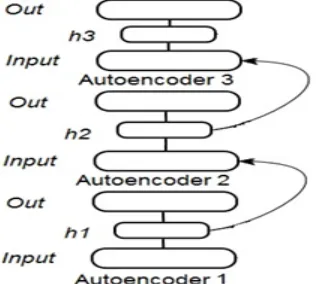
3.2.2. DSAE model
Stacking autoencoders take the output of the previous layer as the next layer input. More clearly, suppose there is a DSAE with H hidden
layers. The first hidden layer h1 is trained as an
autoencoder with the input training set. The
learned features by h1 are taken as an input to the
second autoencoder h2. Then, the learned features
by h2 are taken as an input to the third
autoencoder h3 and with the same way all above
hidden layers, as shown in Fig. 5.
Input: data samples.
Method:
1) Load an input x ∈ R and us a deterministic
function based on (7) to map this input to the
latent representation h ∈ R .
h f σ Wx b (7)
where R is a set of real numbers, W is d× d
weight matrix, b is a dimensionality offset
vector d , and θ = {W, b}.
2) Apply a reverse mapping according to (8) to
reconstruct the input.
f: y f h σ Wh b (8)
3) Set the two weight sets to be in the form W =
W and use them for encoding the input and
decoding the latent representation.
4) With the same way, map each training unit x
onto its code h and its reconstruction y.
5) Adjust the parameters and minimize the
appropriate cost function over the training set
D x , t , … , x , t .
Output: reconstruction of the input samples. Algorithm1: The encoding and decoding processes of
autoencoders.
Figure 5: The stacked autoencoder architecture.
To make use of the learned features in classification tasks, a predictor layer is added to the stacked autoencoders. This layer is usually
[image:9.612.320.530.97.464.2]called softmax layer. Softmax is a linear classifier that uses the cross-entropy loss function (see equation (9)) to create a regular likelihood distribution on the outputs [33]. Cross-entropy loss function minimizes the mean of the error for the model predictions on a certain training set and hints to faster convergence. The stacked autoencoder plus the softmax layer cover the proposed deep architecture model, as shown in Fig. 6.
z ∑ (9)
where ythe total weighted sum of inputs to the
output unit i and k is the number of classes.
Figure 6: The proposed DSAE network.
Training DSAE with using classical methods, such as back-propagation, has essential problems [34]. The leverage of back-propagated errors on the first layers becomes infinitesimal and relatively ineffective when the NN composed several nonlinear transformation layers. For this reason, the deep network uses additional progressive back-propagation approaches, such as the conjugate gradient scheme, to be able to learn how to rebuild the average of all the training data [35]. However, it is found that training the deep networks by this way leads to very slow training with poor solutions. To avoid these problems, we suggest greedy layer-wise unsupervised learning algorithm to train the DSAE network.
[image:9.612.118.276.530.672.2]5916 as an input. After pre-training all layers, the parameters of the whole network can be fine-tuned in a top–down way to minimize reconstruction er-rors due to unsupervised mode. Back-propagation supervised learning algorithm is usually used in a fine-tuning stage.
We can make use of greedy layer-wise unsupervised learning algorithm in training DSAE by applying the following steps [37]:
1. The first hidden layer is trained as an
autoencoder by underestimating the objective function with the input training set.
2. The output of the first hidden layer is used as
an input to the second hidden layer then the second hidden layer is trained as an autoencoder.
3. For training, the desired number of hidden
layers, iterate step 2.
4. The output of the last hidden layer is used as
the input for the top prediction layer, and its parameters are initialized randomly or by supervised training.
5. Back-propagation algorithm is applied in a
supervised manner to fine-tune the parameters of the whole network.
The pseudo-code for training and fine-tuning DSAE is presented in Algorithms 2 and 3.
Algorithm 2: The pre-training of DSAE.
4. EXPERIMENTAL RESULTS AND DISCUSSION
Algorithm 3: The fine-tuning of DSAE.
4. EXPERIMENTAL RESULTS 4.1. Data Set Description
The used data set is the PAMAP2 Physical Activity Monitoring data set [38, 39]. The PAMAP2 holds records of 18 different physical activities. These activities are lying, sitting, standing, walking, running, cycling, Nordic walking, watching TV, computer work, car driving, ascending stairs, descending stairs, vacuum cleaning, ironing, folding laundry, house cleaning, playing soccer, and rope jumping. Nine subjects (one female, eight males) are contributed to the data collection by wearing 3 Colibri
Input: D: Training set,D x , y
ε: Learning rate for pre-training
Method:
Initialize weights W // weight from jth unit
to kth unit in ith layer.
Set biases bto zero.
For i {1, …, I} do
While stopping condition of pre-training is not met
For each training input example X
Do
X → h x
for j {1,...,i − 1} do
a(x)=b+W h x
h x σ a x
End for
Use h x as input unit
Update weights W
Update biases b , b
End while End for
Input: x: Training input.
W: Autoencoder weights.
b , b: Biases
ε : Learning rate for fine-tuning
Method:
Set autoencoder parameters
W → W b → b
b → c
Go forward:
a(x) ← b+ W
h(x) ← σ (a(x))
a(x) ← c+ W h(x)
x ← σ (a(x)) Go backward:
∂C x, x
∂a x ← x x
∂C x, x
∂h x ← W
∂C x, x ∂a x
∂C x, x
∂a x ←
∂C x, x
∂h x h x 1
h x for j ∈ 1, . . . , |h x |
Update network parameters:
W ← W ε ∂C x, x
∂a x X
h X ∂C x, x
∂a x
b ← b ε∂C x, x
∂a x
b ← b ε∂C x, x
5917 wireless inertial measurement units (IMUs) and a heart rate monitor. The first IMU was worn over the wrist on the dominant arm. The second IMU was worn on the chest. The third was worn on the dominant side's ankle. Each IMU had a sampling frequency of 100Hz, so data was given every 0.01s. The PAMAP2 data set converged approximately 3850505 instances with 54 features. These features were a timestamp, activityID, heart rate, 17 features for IMU hand sensory data, 17 features for IMU chest sensory data, and 17 features for IMU ankle sensory data. Table 1 summarizes the characteristics of PAMAP2 data set subjects.
Table 1: Characteristics of the PAMAP2 data set.
We carried out the proposed system on the PAMAP2 data set using Waikato Environment for Knowledge Analysis (Weka) version 3.8.0 [40], Rapidminer 7.0.1, and Matlab 2016b running on a laptop with an AMD A6, 2.3 GHz processor, HD graphic, and 4 GB RAM.
4.2. Data set preparation
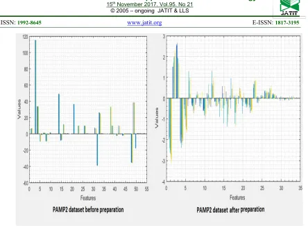
First, a reduced representation for PAMAP2 data set with only 34 features is obtained, when we applied interval-valued fuzzy rough feature selection methodology. Then, all NAN values in the data set are replaced by their maximum likelihood using the EM algorithm. Second, outliers are detected using KNN. K value is adjusted to 100. Choosing a large value for K helps in detecting the overall noise in the data. Depending on the detection results, all instances with true outlier value are removed. Finally, we train SOM network with learning rate equal to 0.8 and train it with up to 50 rounds. A Low-dimensional view of data is obtained after training the network. Fig. 7 shows the differences between the distribution of PAMAP2 data set before and after preparation.
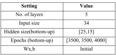
4.3. DSAE Setting
[image:11.612.324.522.384.479.2]As any neural network, the variables of the network depend on the problem itself. To select our network structure that will give the best performance, we trained the network repeatedly with random values. After training attempts, we found that the best architecture is built from a DSAE model with five layers: an input layer, two hidden layers, softmax layer, and an output layer. The input layer carries the data set features, so its size is 34. The hidden layers sizes are regulized to be smaller than the dimension of the input units to be able to extract more valuable features. So, we adjust the first hidden layer size to be 25 and the second hidden layer size to be 15. The best performance is observed after 3500 epochs for each hidden layer and after 4000 epochs for the softmax layer. Table 2, summarizes the setting of the proposed the DSAE model.
Table 2: The structure of the DSAE for the PAMAP2 data set classification.
Setting Value
No. of layers 5
Input size 34
Hidden size(bottom-up) [25,15] Epochs (bottom-up) [3500, 3500, 4000]
Wx,b Initial
We train the DSAE with only 50% of the data and use the remaining as a test data. The purpose of this cross-validation is to make use of the ability of deep networks in dealing with large volumes of unlabeled data. The DSAE is trained one layer at a time in a greedy layer-wise manner. The first hidden layer is trained as an autoencoder by underestimating the objective function with the input training set. The output of the first hidden layer is used as an input to the second hidden layer, which is also trained as an autoencoder. The output of the second autoencoder is used as the input for the top softmax layer, and its parameters are initialized randomly. Finally, a back-propagation algorithm is applied in a supervised manner to fine-tune the parameters of the whole network.
Subject
No. instances No. of
No. of missing
values
Anomalies Range
1 376417 397958 ~52%
2 447000 500742 ~53%
3 252833 250681 ~55%
4 329576 359437 ~55%
5 374783 405721 ~44%
6 361817 375280 ~51%
7 313599 332553 ~54%
8 408031 462822 ~52%
5918
Figure 7: The reduced representation for PAMAP2 data set after preparation.
4.4. Results
We tested the classification performance of the DSAE in terms of accuracy, specificity, and sensitivity. Accuracy is the percentage of correctly classified samples and can be calculated by using equation (10). Specificity is the true negative rate and can be calculated by using equation (11). Sensitivity is the true positive rate and can be calculated by using equation (12).
Accuracy (10)
Specificity (11)
Sensitivity (12)
where TP is the number of correctly classified samples, FP is the number of incorrectly rejected samples, TN is the number of correctly rejected samples, and FN is the number of incorrectly classified samples.
Table 3 shows the performance of our proposed system before fine-tuning and after
[image:12.612.337.521.523.604.2]fine tuning by applying the back-propagation algorithm to the whole network. It can be observed that the accuracy of the proposed system after fine-tuning the DSAE is higher than the accuracy before fine-tuning. The rise in classification accuracy after fine tuning highlights its importance in training the DSAE.
Table 3: The classification test results for DSAE before and after fine-tuning
Measurements Proposed
system before fine-tuning
Proposed system before fine-tuning
Accuracy 89.20 % 99.8%
Specificity 87.40% 99.9%
Sensitivity 89.260% 99.8%
[image:12.612.101.253.553.624.2]5919 percentage, which is 99.8% for correct predictions and only 0.2% for wrong predictions.
Figure 8: The confusion matrix for the DSAE classifier.
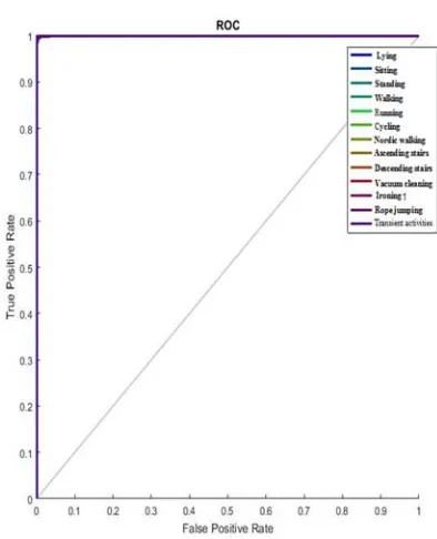
Receiver Operating Characteristic (ROC) curve is shaped by scheming the true positive rate (TPR) against the false positive rate (FPR) at various threshold settings. As the closer, the ROC curve is to the upper left corner, the higher the overall accuracy of the test. Fig. 9 showed ROC curve of the proposed framework that achieves high accuracy (near to 100%) however we used only 50% of the data for training.
[image:13.612.323.520.385.628.2]5920 Table 4: The accuracy of the proposed system with KNN, SVM, and ANN in classifying PAMP2 data set
activities. Classifier
type/ Activity
type
KNN SVM ANN
The proposed
system
Accuracy (%) Transient
activities 99 98.9 96.1 99.8
Lying 89 99 39.4 100
Sitting 99 98 98 99.9
Standing 99 100 99.4 100
Walking 95 98 50.9 100
Runing 100 100 76.2 100
Cycling 97 95 61.9 98
Nordic
walking 99 96 39.1 97
Ascending
stairs 96 95 65.2 100
Descending
stairs 96 98 88 98.6
Vacuum
cleaning 99 98 81.6 99.5
Ironing 99 100 98.6 100
Rope
jumping 96 97 88.4 97.1
To ensure the validity of our proposed system, we compared it with some state-of the-art classifiers. Those classifiers are KNN, SVM, and ANN. We used the same training and testing data during the comparison. Table 4, shows the accuracy of each classifier in recognizing PAMAP2 data set activities. It is observed that our proposed system, which is based on DSAE classifier, achieves the highest percentage of correct predictions compared to tested classifiers. The proposed system achieved an overall accuracy of 99.8% compared with the accuracy of KNN, SVM, and ANN, which are 99.2, 99.3, and 95.2%, respectively.
Fig. 10 shows a diagram that characterizes the overall performance evaluation of the proposed system with KNN, SVM, and ANN. It is proved that our proposed system outperforms the three
state-of-the-art techniques in classifying
PAMAP2 data set.
Figure 10: The performance evaluation of the proposed system.
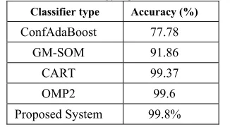
[image:14.612.91.290.102.450.2]On the other hand, Orthogonal Matching Pursuit 2 (OMP2), GM-SOM, classification and regression tree (CART), and ConfAdaBoost classifiers are used in [41, 42] to classify PAMAP2 data set. From the results represented on these works, our proposed system achieves the highest accuracy. The proposed system achieved an overall accuracy 99.8% compared with the accuracy of OMP2, GM-SOM, CART, and ConfAdaBoost, which are 99.6, 91.86, 99.37, and 77.78 % respectively.
Table 5: The accuracy of the proposed system with related work on classifying PAMAP2 data set.
Classifier type Accuracy (%)
ConfAdaBoost 77.78
GM-SOM 91.86
CART 99.37
OMP2 99.6
Proposed System 99.8%
4.5.Discussion
[image:14.612.343.506.504.594.2]5921 be mirrored as a real source of knowledge for tasks of Big Data analytics.
The main factors that aid in reaching to such competing results are:
1- The proposed preprocessing framework
aids in achieving high-quality mining results as quality conclusions must be built from quality data.
2- Using autoencoders as fundamental
building blocks for DSAE improves learning and allows greater depth for
dimensionality reduction and data
encoding.
3- Hieratical Training makes DSAE model
more scalable and powerful than shallow networks.
4- Fine-tuning the whole DSAE network after
training represents the preferred outputs and derivatives of back-propagating errors.
Besides that, our proposed system faced two challenges which are:
1- Adjusting the values of DSAE parameters,
such as the learning rate schedule, the strength of the regularized, the number of layers, and the number of units per layer are trial and error tasks and lead to consuming additional time.
2- The capacity of DL architectures is directly
proportional to the number of hidden units instead of non-parametric forms of their energy function. This will lead to deeper and more complex computations.
5. CONCLUSION
We proposed a system that can work as a key enabler for the large scale of Big Data in IoT. We consider analysis for Big Data IoT faces four challenges: the abundant existence of missing values, the presence of a high range of anomalies in each subject, the high variety of data types, and the massive volumes of data instances. We handled each challenge independently. For the existence of missing values, we firstly apply interval-valued fuzzy-rough feature selection methodology to highlight the most important features that contain missing data and getting rid of the others. Then, we use ML approach for replacing the missing values. For the presence of anomalies, we initially utilize KNN algorithm to detect the unusual patterns that do not belong to normal events. Then, we remove all these patterns from the data. For the nonlinear separability of data, we exploit SOM to obtain low- dimensional
views of the data. After that, we proposed DSAE instead of ANN as a DL-based classifier to provide efficient processing of such volumes of data. We evaluate our proposed model in the PAMAP2 data set, and results show that DSAE is truthfulness classifier for IoT Big Data. The advantage of the proposed system is that the extracted features by the DSAE are non-handcrafted and task dependent, which gives it the most discriminative power to work as an efficient DL classifier for representing a high-level abstraction of IoT data while the drawback is that the training phase of DSAE is a time-consuming task.
For future work, it would be remarkable to examine hybrid DL algorithms for large scale sensor data prediction and to evaluate these algorithms on different open public IoT data sets to inspect their efficiency. Finally, we also tend to concentrate on remain challenges of IoT Big Data, which are velocity and variety.
REFERENCES
[1] C. Cecchinel, M. Jimenez, S. Mosser, and M. Riveill, An Architecture To Support The Collection Of Big Data In The Internet Of
Things, In the proceedings of the IEEE 10th
World Congress On Services, 2014, pp. 442-449.
[2] N. Lane, S. Bhattacharya, P. Georgiev, C. Forlivesi and F. Kawsar, An Early Resource Characterization of Deep Learning on Wearables, Smartphones and Internet-of-Things Devices, In the proceedings of the 2015 International Workshop on Internet of Things towards Applications, November 01-01, Seoul, South Korea, 2015), pp. 7-12. [3] Y. Xu, Recent Machine Learning Applications
to Internet of Things (IoT), Recent advances in networking, [online] Available at: http://www.cse.wustl.edu/~jain/cse570-15/index.html (Last accessed on 3/8/2016). [4] Y. Lv, Y. Duan, W. Kang, Z. Li and F. Y.
Wang, Traffic flow prediction with big data: a deep learning approach, IEEE Transactions on Intelligent Transportation Systems, 2015, pp. 865–873.
[5] J. B. Yang, M. N. Nguyen, P. P. San, X. L. Li and S. Krishnaswamy, Deep Convolutional Neural Networks on Multichannel Time Series for Human Activity Recognition, In
the proceedings of the 24th International Joint
5922 (IJCAI), Buenos Aires, Argentina, 2015, pp. 3995–4001.
[6] M. Najafabadi, F. Villanustre, T. Khoshgoftaar, N. Seliya, R. Wald, and E. Muharemagic, Deep Learning applications and challenges in Big Data analytics, Journal of Big Data 2(1) (2015), 1-21.
[7] X. Chen and X. Lin, Big Data Deep Learning: Challenges and Perspectives, In Access, IEEE, 2014, pp.514-525.
[8] N. M. Elaraby, M. Elmogy, and S. Barakat, Deep Learning: Effective Tool for Big Data Analytics, International Journal of Computer Science Engineering 5(5) (2016), 254-262. [9] H.-C. Shin, M. R. Orton, D. J. Collins, S. J.
Doran and M.O. Leach, Stacked
autoencoders for unsupervised feature learning and multiple organ detection in a pilot study using 4D patient data, IEEE Trans. Pattern Anal. Mach. Intell. 35(8) (2013), 1930–1943.
[10] C. Paniagua, H. Flores and S. Srirama, Mobile Sensor Data Classification for
Human Activity Recognition using
MapReduce on Cloud, In the proceedings of
the 9th International Conference on Mobile
Web Information Systems, Procedia
Computer Science 10 (2012), 585 – 592. [11] P. Gajdos, P. Moravec, P. Dohnalek, and T.
Peterek, Mobile Sensor data classification using gm som, Adv. Intell. Syst. Comput. 210(1) (2013), 487–496.
[12] D. Anguita, A. Ghio, L. Oneto, X. Parra and J. Reyes-Ortiz, A Public Domain Dataset for
Human Activity Recognition Using
Smartphones. 21st European Symposium on
Artificial Neural Networks, Computational
Intelligence, and Machine Learning,
ESANN, Bruges, Belgium, 2013, pp. 437-442.
[13] W. Dai, and W. Ji, A MapReduce Implementation of C4.5 Decision Tree Algorithm, International Journal of Database Theory and Application 7(1) (2014), 49-60. [14] E. Coninck, T. Verbelen, B. Vankeirsbilck,
S. Bohez, P. Simoens, P. Demeester, and B. Dhoedt, Distributed neural networks for Internet of Things: the Big-Little approach,
2nd EAI International Conference on
Software Defined Wireless Networks and Cognitive Technologies for IoT, 2015, pp. 1 – 9.
[15] A. Shilton, S. Rajasegarar, C. Leckie, and M. Palaniswami, Dp1svm: A dynamic planar one-class support vector machine for the internet of things environment, In the proceedings of the International Conference on Recent Advances in Internet of Things (RIoT), 2015, pp. 1–6.
[16] R. Chettri, S. Pradhan, and L. Chettri, Internet of Things: Comparative Study on Classification Algorithms (k-NN, Naive
Bayes and Case-based Reasoning),
International Journal of Computer
Applications 130(12) (2015), 7-9.
[17] J. B. Yang, M. N. Nguyen, P. P. San, X. L.
Li, and S. Krishnaswamy, Deep
Convolutional neural networks on
multichannel time series for human activity
recognition, In the proceedings of the 24th
International Joint Conference on Artificial
Intelligence (IJCAI), Buenos Aires,
Argentina, 2015, pp. 25–31.
[18] L. Mo, F.an Li, Y. Zhu, A. Huang, Human physical activity recognition based on computer vision with deep learning model, IEEE International Instrumentation and
Measurement Technology Conference
Proceedings 30(3) (2016), 1-6.
[19] F. J. Ordóñez and D. Roggen, Deep Convolutional and LSTM Recurrent Neural Networks for Multimodal Wearable Activity Recognition, Sensor Technology Research Centre, 2016.
[20] M. A. Alsheikh, D. Niyato, S. Lin, H.P. Tan, and Z. Han, Mobile Big Data Analytics Using Deep Learning and Apache Spark, arXiv preprint arXiv: 1602.07031, 2016.
[21] R. Jensen and Q. Shen, Interval-valued Fuzzy-Rough Feature Selection in Datasets with Missing Values, In the proceedings of
the 18th International Conference on Fuzzy
Systems, 2009, pp. 610–615.
[22] M. Kumar and N. Yadav, Fuzzy-Rough Sets and Its Application in Data Mining Field, Advances in Computer Science and Information Technology (ACSIT) 2(3) (2015), 237-240.
5923 [24] A. Farhangfar, L. Kurgan, and J. Dy, Impact
of Imputation of Missing Values on Classification Error for Discrete Data Pattern Recogn, Elsevier Science Inc 41(12) (2008), 3692-3705.
[25] A. N. Baraldi and C.K. Enders, An introduction to modern missing data analyses, Society for the Study of School Psychology, 48 (2010), 5–37.
[26] I. Witten, and E. FranK, Data Mining: Practical machine learning tools and techniques, Morgan Kaufmann, Second Edition, 2005, pp. 1-525.
[27] K. Chomboon, P. Chujai, P. Teerarassamee, K. Kerdprasop, and N. Kerdprasop, An Empirical Study of Distance Metrics for k-Nearest Neighbor Algorithm, In the
proceedings of the 3rd International
Conference on Industrial Application Engineering, 2015, pp. 280-285.
[28] P. Campoy, Dimensionality Reduction by Self-Organizing Maps that preserve distances in Output Space, In the proceedings of the International Joint Conference on Neural Networks, Atlanta, Georgia, USA, 2009, pp. 432-438.
[29] Ng. Andrew, Sparse auto encoder, CS294A Lecture Notes: Stanford University, 2011. [30] S. Rifai, P. Vincent, X. Muller, X. Glorot,
and Y. Bengio, Contracting auto-encoders: Explicit invariance during feature extraction, In ICML, 2011.
[31] J. Masci, U. Meier, D. Ciresan, and J. Schmidhuber, Stacked Convolutional auto-encoders for hierarchical feature extraction, In the proceedings of the 21st International
Conference on Artificial Neural Networks 1(11) (2011), 52–59.
[32]P. Vincent, H. Larochelle, I. Lajoie, Y. Bengio and P.-A. Manzagol, Stacked Denoising Autoencoders: Learning useful representations in a deep network with a local denoising criterion, In the proceedings of the
27th International Conference on Machine
Learning, ACM, 2011, pp. 3371–3408. [33] L. G. Hafemann, An analysis of deep neural
networks for texture classification, M.Sc. program in Informatics, Universidade Federal do Paran'a, 2014.
[34] L. Deng, A tutorial survey of architectures, algorithms, and applications for Deep Learning, in APSIPA Transactions on Signal and Information Processing, 2014.
[35] G. E. Hinton, S. Osindero, and Y. Teh, A fast learning algorithm for deep belief nets, Neural Computation 1(18) (2006), 1527-1554.
[36] L. Arnold, S. Rebecchi1, S. Chevallier1, and H. Moisy, An Introduction to Deep Learning, In the proceedings of the European Symposium on Artificial Neural Networks (ESANN 2011), Computational Intelligence, and Machine Learning, 2011.
[37] H. Larochelle, Y. Bengio, J. Louradour, and P. Lamblin, Exploring strategies for training deep neural networks, Journal of Machine Learning Research, 2012.
[38] A. Reiss and D. Stricker, Introducing a New
Benchmarked Dataset for Activity
Monitoring, In the proceedings of the 16th
IEEE International Symposium on Wearable Computers (ISWC), 2012, pp. 108-109. [39] A. Reiss and D. Stricker, Creating and
Benchmarking a New Dataset for Physical Activity Monitoring, In the proceedings of
the 5th Workshop on Affect and Behaviour
Related Assistance (ABRA), 2012.
[40] R. Jensen, N. Parthaláin, and Q. Shen,
Tutorial: Fuzzy-Rough data mining,
[Online]. Available at:
http://users.aber.ac.uk/rkj/wcci-tutorial-2014, 2014 (last accessed on 1/8/2017). [41] P. Dohnálek, P. Gajdoš, P. Moravec, T.
Peterek, and Václav Snášel, Application and comparison of modified classifiers for human
activity recognition, PRZEGLĄD
ELEKTROTECHNICZNY, 2013, pp. 55-58. [42] A. Reiss, D. Stricker, and G. Hendeby, Confidence-based Multiclass AdaBoost for Physical Activity Monitoring, In the
proceedings of the IEEE 17th International