OPTIMIZATION STUDY OF RSI EXPERT SYSTEM BASED
ON SHANGHAI SECURITIES MARKET
HUANG HAI-PING, WANG PIN
Mathematics and Computer Science Department, Guangxi College of Education, Nanning, Guangxi,
530023, China
*Corresponding author:
WANG PINABSTRACT
Through the simulation experiment method, by means of general securities information and trading platform in Mainland China, based on the historical data of all A shares in Shanghai Securities Market within 16 years, with the winning rate, the annual rate of return, and the net profit as the goal, and through detecting the current general RSI expert trading system, the article corrected the trading points of RSI trading system and achieved the result of maximized goal.
Keywords: Simulation Experiment, Historical Data, Winning Rate, Annual Rate of Return, RSI Trading
System
1. INTRODUCTION
In the securities investment market, three results that all investors are most concerned about are the winning rate (the ratio between the transaction number of earnings and the total transaction number), the annual rate of return and the net profit margin, the higher winning rate means the less risk for investors, the higher annual rate of return means the more profits for investors, and the higher net profit margin means the faster that the investors can make money. In the current global financial transactions, as commonly recognized, there are two mature methods: fundamental analysis and technical analysis. During the technical analysis method, the technical indicators must be used.
RSI (Relative Strength Index) trading indicator is mentioned in 1978 by U.S. J.Welles Wilder, JR. in the book "New Concepts in Technical Trading Systems [1]", and the corresponding formula is given out. Subsequently, RSI indicator is widely used in the global trading of commodities, futures, and securities. Domestic researchers have also done a lot of work and achieved many beneficial results.
JIAO Hua (2001) [2] discussed the mathematical meaning of RSI (6) calculation formula and proposed its mathematical explanation.
GAO Xiang-bao, ZHAO Ying-jie (2005) [3] studied the historical weekly data of Shanghai Composite Index from 1992 to 2005. With Shanghai Composite index as the investment products, the strategy of closing the position in
batches was applied, and the conclusion was drawn
that the average profit is largest at 70 ≤ RSI (6) ≤
80.
CHENG Jin-bo (2006) [4] studied the historical weekly data of Shanghai Composite Index from 1992 to 2006. With Shanghai Composite index as the investment products, it drew the probability
when 10 ≤ RSI (6) ≤ 20 is at the bottom and the
probability when 80 ≤ RSI (6) ≤ 90 is at the top.
TAO Cui (2007) [5] used the Monte Carlo simulation method to test the effectiveness of RSI indicator, and the conclusion was that the guiding role of RSI (5) in the stock trading is debatable which needs to be further improved and perfected.
LI Yi-long (2010) [6] described the general application of RSI (14) during the firm bid and ask quotations.
Due to the popularity of computer use, all securities analysis and trading of securities investors can be done through the computer. At present, all securities analysis trading softwares in China incorporated an expert RSI trading system, and this article attempts to test and analyze the relevant historical data in Shanghai and Shenzhen
Securities Markets through the simulation
securities market. It is to seek the optimal trading point with maximized goal, thus to optimize the expert RSI trading system. Writing out the source code of optimization formula, it provides a graphical and intuitive tool to investors.
2. EMPIRICAL ANALYSIS OF RSI
TRADING SYSTEM
2.1 Experiments and Results
The original formula given by Welles Wilder is as follows:
RSI = 100 × RS / (1 + RS) or, RSI = 100-100 ÷ (1 + RS)
Of which, RS = the average of sum of rising numbers in closing price within N days / the average of sum of falling numbers in closing price within N days .
Parameter N is determined by the trader, and Welles Wilder took N = 14 [7]. In securities analysis trading software of Chinese mainland, it was taken at N = 6, 12, 24. In order to obtain the appropriate data, we conducted the simulation experiments as follows:
(1) Experiment platform: Great Wisdom Securities Information Platform V5.98 version
(2) Experiment procedure
LC:=REF(CLOSE,1);
WRSI:=SMA(MAX(CLOSE-LC,0),N,1)/SMA(ABS(CLOSE-LC),N,1)*100;
ENTERLONG:CROSS(WRSI,LL);
EXITLONG:CROSS(LH,WRSI);
(3) Experiment parameters: To take a position of all funds by one time, to close all positions when meeting the sell condition, the transaction cost is taken as 0.5%, LL takes 20 [8] at the beginning, LH = 80 with the step length of 5.
(4) Experiment samples: All A shares (1996.3-2012.9) in Shanghai and Shenzhen Securities Markets.
(5) Experiment process, time and results: See Schedule 1
With the test on Shanghai Securities Market from March 1, 1996 to June 30, 2001 as the example, through the test by test system of Great Wisdom Securities Information Platform V5.98 version, the results are as follows:
Test System Configuration Test methods: technical indicator - RSI14 Test time :1996-3-1 - 2001-6-30 calculation of forced liquidation
Test stocks: total 940 stocks Initial investment: Yuan 40,000.00
Buy conditions:
Once established of one of the following groups: 1. Following conditions are established at the same time
1.1 Technical indicator: the index line RSI of RSI14 (14) pierced upward the 20.00 [daily line] When the conditions are met: according to the mid-price: all funds are used to buy at the closing price
Once a continuous signal: no longer buy in. Sell conditions: no sell conditions
Close-out conditions: (close-out according to the closing price)
Stock selection by indicators: Technical specifications: the index line RSI of RSI14 (14) pierced downward the 80.00 [daily line]
System Test Report Number of testing stocks: 940
Net profit: 9,962,316.00 Yuan Net profit margin: 26.50%
Total earnings: 10,220,472.00Yuan Total loss: -258,195.20 Yuan
Number of transactions: 427 winning rate: 88.99%
Average annual number of transactions: 81.33 Profit/loss transaction number: 380/47 Total turnover: 18,431,974.00 Yuan Transaction fee: 4,784.18 Yuan
Largest single earnings: 173,716.23 Yuan Largest single loss: -16,596.16 Yuan
Average earnings: 23,935.53 yuan Average loss: -604.67 Yuan
Average profit: 23,330.95 Yuan Average earnings/average loss: -3,958.43
Maximum number of consecutive earnings: 42 Maximum number of consecutive losses: 2
Average number of trading cycles: 280.15 Average cycle of profitable transactions: 284.52 Average cycle of loss transactions: 244.77
Earnings coefficient: 0.95
loss: 47,609,844.00 Yuan
Total investment: 37,600,000.00 Yuan Statistics of buy signal
(The statistics of all buy signal points, without considering the signal deletion caused by the capital and strategy during transaction testing)
Success rate: 89.07%
Number of signals: 439 Average annual number of signals: 83.62
Test data in Shanghai Securities Market
LL Winnin g Rate
Annual Rate of Return
Net Profit Margin
Annual Transact ion Number
20 88.94 5.06 26.14 82.26
25 90.68 10.20 52.68 141.29
30 90.33 16.62 85.88 202.06
35 89.43 20.28 104.78 241.74
40 88.23 22.16 114.51 264.77
45 87.20 25.05 129.43 288.77
50 86.63 26.84 138.69 312.77
55 85.82 25.58 132.15 323.42
60 85.39 24.76 127.92 333.87
65 85.50 23.40 120.89 340.45
70 85.36 19.85 102.56 347.61
75 87.54 13.67 70.61 355.74
80 76.35 2.49 12.87 353.61
2.2 Numerical Analysis
SPSS software is used to conduct the regression analysis for the above test data in Shanghai Securities Market, and the results are as follows:
1996.03—2001.06 Winning Rate Analysis Model Summary and Parameter Estimates
Dependent Variable: VAR00002
Equation
Model Summary Parameter Estimates
R Square F df1 df2 Sig. Constant b1 b2 b3 Cubic .965 73.072 3 8 .000 76.418 1.176 -.031 .000
The independent variable is VAR00001.
The above table shows that: R-squared R = 0.965, significance value sig = 0.000. Because the accuracy of coefficient b3 at cubic item is not
enough, MATLAB software is used for re-fitting (cubic polynomial fitting), the fitting function
2 3
77.34727 1.098118
0.028971
0.000214
y
=
+
x
−
x
+
x
, and the function image is shown in Figure 1.
1996.03—2001.06 Annual Return Rate Analysis
Model Summary And Parameter Estimates
Dependent Variable: VAR00002
Equation
Model Summary Parameter Estimates
R Square F df1 df2 Sig. Constant b1 b2 Quadratic .965 138.671 2 10 .000 -35.899 2.470 -.024
The independent variable is VAR00001. The above table shows that: R-squared R = 0.965, significance value sig = 0.000, fitting function
2
35.899 2.47 0.024
y= − + x− x ,and the function
image is shown in Figure 2.
30 .0 0
2 5 .0 0
2 0 .0 0
1 5 .0 0
1 0 .0 0
5. 00
0. 00
8 0 .0 0 70 . 00 60 .0 0 5 0. 00 40 .0 0 3 0 .0 0 2 0 .0 0
VAR 0 0 0 0 2 VAR 0 0 0 0 2VAR 0 0 0 0 2 VAR 0 0 0 0 2
1996.03—2001.06 Net Profit Analysis Model Summary And Parameter Estimates
Dependent Variable: Var00002
Equation
Model Summary Parameter Estimates
R Square F df1 df2 Sig. Constant b1 b2 Quadratic .965 138.835 2 10 .000 -185.500 12.764 -.126
The independent variable is VAR00001.
The above table shows that: R-squared R = 0.965, significance value sig = 0.000, fitting function
2
185.5 12.764 0.126
y= − + x− x , and the function image is
shown in Figure 3.
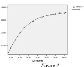
1996.03—2001.06 Annual Transaction Number Analysis Model Summary And Parameter Estimates
Dependent Variable: Var00002
Equation
Model Summary Parameter Estimates
R Square F df1 df2 Sig. Constant b1 b2 b3 Cubic .998 1752.317 3 9 .000 -301.148 25.481 -.346 .002
The independent variable is VAR00001.
The above table shows that: R-squared R=0.998, significance value sig = 0.000, fitting function
2 3
301.148 25.481
0.346
0.002
y
= −
+
x
−
x
+
x
,and the function image is shown in Figure 4.
1 40 . 00 1 20 . 00 1 00 . 00 8 0 .0 0 6 0 .0 0 40 .0 0 2 0 .0 0 0 .0 0
8 0 .0 0 7 0. 00 6 0 .0 0 5 0. 00 40 . 00 3 0. 00 2 0 .0 0
VAR 0 0 0 0 2 VAR 0 0 0 0 2VAR 0 0 0 0 2 VAR 0 0 0 0 2
Figure 3 Figure 4
For the fitting function of winning rate analysis
2 3
77.34727 1.098118 0.028971 0.000214
y= + x− x + x , we
can obtain the stationary points x1=63.184, and
068 . 27
2=
x . As shown in Figure 3, the maximum
point x=27.068.
For the fitting function of annual return rate
analysis 2
35.899 2.47 0.024
y= − + x− x , when
2.47 0.048
y′ = − x and y′′=−0.048, it obtained:
0
048
.
0
47
.
2
−
x
=
, and the maximum point46 . 51 = x .
Similarly, for the fitting function of net profit
analysis, we obtained the maximum point x=50.65.
As shown by the fitting function of annual
transaction number analysis
2 3
301.148 25.481 0.346 0.002
[image:4.612.320.466.362.479.2]y= − + x− x + x and its image
Figure 4, y is the monotonically increasing function of x.
Time Function LL Maximum Point
1996.03 ~ 2001.06
2 3
77.34727 1.098118 0.028971 0.000214
y= + x− x + x
2
35.899 2.47 0.024
y= − + x− x
2
185.5 12.764 0.126
y= − + x− x
2 3
301.148 25.481 0.346 0.002
y= − + x− x + x
27.07 51.46 50.65
Monotonically increasing function
2001.07 ~ 2005.06
2
43.493 1.251 0.017
y= − x+ x
2
1.523 0.582 0.007
y= − x+ x
2
5.978 2.282 0.026
y= − x+ x
2 3
251.332 4.185 0.240 0.003
y= − x+ x − x
36.79(Minimum point) 41.57(Minimum point) 43.88(Minimum point) 42.35
2005.07 ~ 2007.09
2 3
82.9002 1.2512 0.0310 0.0002
y= + x− x + x
2
2005.724 115.137 1.173
y= − + x− x
2 3
152.015 55.376 2.810 0.028
y= − x+ x − x
2 3
1797.012 115.605 1.508 0.007
y= − + x− x + x
27.4983
49.08 54.89
Monotonically increasing function
2007.10 ~ 2008.12
2
41.896 1.398 0.019
y= − x+ x
2
24.997 2.373 0.024
y= − x+ x
2
29.1614 2.768 0.028
y= − x+ x
2 3
1366.696 112.26 1.630 0.006
y= − + x− x + x
36.79(Minimum point) 49.44(Minimum point) 49.43(Minimum point)
46.24
2009.01 ~ 2009.12
2
83.643 0.613 0.008
y= + x− x
2
265.291 15.055 0.145
y= − + x− x
2
243.188 13.801 0.133
y= − + x− x
2 3
1038.922 25.439 1.386 0.017
y= − + x+ x − x
38.31 51.92 51.88 62.35 2010.01 ~ 2010.06 2 3
27.305 3.269 0.083 0.001
y= − + x− x + x
2
44.922 3.055 0.03
y= − x+ x
2
18.724 1.273 0.012
y= − x+ x
2 3
4867.703 348.607 5.174 0.021
y= − + x− x + x
Monotonically increasing function 50.92(Minimum point) 53.04(Minimum point)
47.32
2010.07 ~ 2011.03
2
71.966 0.905 0.014
y= + x− x
2
92.508 6.274 0.066
y= − + x− x
2
61.679 4.183 0.044
y= − + x− x
2 3
3477.173 234.654 3.272 0.013
y= − + x− x + x
32.32 47.53 47.54 51.93 2011.04 ~ 2012.09 2
71.966 2.445 0.026
y= − x+ x
2 3
62.019 4.305 0.07 0.000327
y= − x+ x − x
2 3
87.84 6.098 0.099 0.00046
y= − x+ x − x
2 3
709.227 75.369 1.081 0.004
y= − + x− x + x
47.02(Minimum point)
44.84(Minimum point)
44.76(Minimum point)
47.26
2.3 Market Analysis of Mathematical Results As shown from the quarterly closing line of Shanghai Composite Index in Shanghai Securities Market (see Figure 5), the quarterly closing line of
Figure 5
Mathematical Results In Bull Market
Time Market Rise(
%)
Maximum Point of Winning Rate
Maximum Point of Annual Return
Rate
Maximum Point of Net Profit Margin
Maximum Point of Annual Transaction
Number
1996.03~2001.06 298.04 27.07 51.46 50.65 Monotonically
increasing function
2005.07~2007.09 413.65 27.49 49.08 54.88 Monotonically
increasing function
2009.01~2009.12 80.05 38.31 51.92 51.88 62.3527
2010.07~2011.03 22.09 32.32 47.53 47.54 51.9285
As shown in the above results, in the bull market state, the average maximum point for winning rate is: 31.30; the average maximum point for annual rate of return is: 50.00; the average maximum point for net profit margin is: 51.23; the average maximum point for annual transaction number is: 57.14, or the function of annual transaction number is the monotonically increasing function. Its market implication is that, there is the largest winning rate (least lose) for buy stocks when the RSI pierced upward 31.30; the annual rate of return for buy
stocks is the largest (the most profitable) when the RSI pierced upward 50.00 ; When RSI pierced upward 51.23, the annual net profit margin for buy stocks is the largest (fastest profit). When the RSI pierced upward 57.14 or RSI value is increasing, the success rate of transactions becomes larger. It means that, at this time the stock market is a strong market, and the RSI value keeps always in the higher range.
Mathematical Results In Bear Market
Time Market Rise(
%)
Maximum Point of Winning Rate
Maximum Point of Annual Return
Rate
Maximum Point of Net Profit Margin
Maximum Point of
Annual Transaction
Number
2001.07~2005.06 -51.26 36.79
(Minimum point)
41.57 (Minimum point)
43.88 (Minimum point)
42.35
2007.10~2008.12 -67.21 36.79
(Minimum point)
49.44 (Minimum point)
49.43 (Minimum point)
46.24
2010.01~2010.06 -26.82 Monotonically
increasing function
50.92 (Minimum point)
53.04 (Minimum point)
47.32
2011.04~2012.09 -28.75 47.02
(Minimum point)
44.84 (Minimum point)
44.76 (Minimum point)
As shown from the above results, the winning rate, the annual rate of return, and the net profit margin have no maximum points and have only minimum points in the bear market state. The average minimum point for winning rate is: 40.20; the average minimum point for annual rate of return is: 46.69; the average minimum point for net profit
margin is: 47.78; the average maximum point for annual transaction number is: 45.79.
With the time period from 2007.10 to 2008.12 as an example, the fitting function images for winning rate, annual rate of return, and net profit margin are listed below (see Figure 6, Figure 7, Figure 8, Figure 9)
Figure 6 Figure 7
Figure 8 Figure 9
As shown in Figure 6: when 0≤RSI≤36.79,
the winning rate is the decreasing function of RSI, its market implication is that: the greater the RSI value, the fewer number of investment profitability;
while 36.79≤RSI≤85, the winning rate is the
increasing function of RSI, and its market implication is that, the greater the RSI value, the more number of investment profitability;
As shown in Figure 7 and Figure 8: when
0≤RSI≤50, the annual rate of return and the net
profit margin are the decreasing function of RSI and are negative, its market implication is that: the greater the RSI value, the smaller the annual investment rate of return and the net profit margin,
i.e. the greater the loss. When 50≤RSI≤80, the
annual rate of return and net profit margin are the increasing function of RSI and are negative, its
market implication is that: the greater the RSI value, the greater the annual investment rate of return and the net profit margin, i.e. the smaller the loss but still in a loss.
As shown in Figure 9: the maximum point of annual transaction number is 46.24, its market implication is that: the number of transaction
success is the largest. When 46.24≤RSI ≤90, the
annual transaction number is the decreasing function of RSI, and its market implication is that: the greater the RSI value, the fewer number of transaction success.
In summary, from the perspective of investment profit, the RSI expert system can not guide the investors to profit in bear market.
LC:=REF(CLOSE,1);
WRSI:=SMA(MAX(CLOSE-LC,0),N,1)/SMA(ABS(CLOSE-LC),N,1)*100; ENTERLONG:CROSS(WRSI,LL);
EXITLONG:CROSS(LH,WRSI);
The following Figure 10 and 11 are respectively the image of the same stock before and after optimizing the RSI indicator, and the earnings result in Figure 11 is obviously better than in Figure 10.
Figure 10 Figure 11
3. CONCLUSION
This article takes the winning rate, the annual rate of return, and the net profit as management objectives, using the method of simulation experiment, on the basis of historical data of all A shares in Shanghai Securities Market within 16 years, it obtained the RSI value (buy points) with maximizing goal and the optimized source code of RSI expert system. As a result, it provides all investors with a visual indicator. The results of this study are obtained under unchanged LL value, and the follow-up study will consider the RSI expert system optimization when LL value changes (i.e. the extremum of binary function). We believe that, solving by using the extremum of multi-variable function, we can find the effective RSI expert system under the bear market state.
REFRENCES:
[1] New Concepts in Technical Trading Systems -
J.Welles Wilder. 1978
[2] JIAO Hua, Discussions on RSI Technical
Indicators, Journal of Guizhou Commercial College, 2001
[3] GAO Xiang-bao, ZHAO Ying-jie. Securities
Sell Statistical Decision Based on RSI, Statistics & Decision, 2005
[4] CHENG Jin-bo, Securities Sell Statistical
Decision Based on RSI. Techno-economic Market. 2006
[5] TAO Cui, Applying Monte Carlo Simulation
Method to Test the Effectiveness of RSI Indicator, Finance and Economy, 2007
[6] LI Yi-long, Preliminary Study on the
Application of Relative Strength Index in Shanghai and Shenzhen Securities Markets, Economic & Trade Update, 2010
[7] WANG Zhao-jun, The Best Parameter
Portfolio of RSI. Mathematics in Economics, 2001
[8] WANG Yuan, FANG Kai-tai, About the