CLASSIFICATION OF ECG BEATS USING FEATURES
FROM TWO-STAGE TWO-BAND WAVELET
DECOMPOSITION
1
U.CHANDRASEKHAR, 2LAXMI DHAR DWIVEDI, 3CHIRANJI LAL CHOWDHARY
1
Asstt Prof(Sr), School of Information Technology and Engineering,VIT University, Vellore
2
Asstt Prof(Sr), School of Sciences and Languages,VIT University, Vellore
3Asstt Prof(Sr), School of Information Technology and Engineering,VIT University, Vellore E-mail: [email protected], [email protected], [email protected]
ABSTRACT
The paper focuses on computer aided diagnosis of heart diseases. We extracted QRS complexes of ECG signals from different patients. These ECG signals were decomposed using discrete wavelet transform. Using six different features of ECG signals were able to discriminate and classify six types of heart beats. Three of the features were statistically calculated from decomposed sub band signal. Two more features are taken as AC power and instantaneous RR interval of original signal. The effects of two wavelet decomposition structures, the two-stage two-band and the two-stage full binary decomposition structures, in the recognition of ECG beat types are studied. Either ANN or PNN are found to be useful to classify the features. Results show that two stage two band decomposition is sufficient and we can get very good accuracy by using just 11 features. The reason seems to be that most of the energy is concentrated in the Lower sub bands of the signals. The Higher frequency components do not have any notable information about diseases observable with ECG beat signals.
Keywords: ECG , P-QRS-T waves, Wavelets, feature extraction, PNN
1. INTRODUCTION
The Electrocardiogram ( ECG ) is a diagnostic tool that measures and records the electrical activity of the heart in detail. Interpretation of these details allows diagnosis of a wide range of heart diseases. These signals are within the frequency range of 0.05 to 100 Hertz. The standard parameters of the ECG wave are the P wave, QRS Complex and the T wave. A critical feature of many biological signals is frequency domain parameters. To analyze ECG signals, both frequency and time information is needed simultaneously [7]. Wavelets, which provides for wideband representation of signals, is therefore a natural choice for biomedical engineers. The Discrete Wavelet transform ( DWT ) which is based on sub band coding is found to yield a fast computation of wavelet transform. DWT is computed by successive low pass and high pass filtering of the discrete time-domain signal as shown in Fig-1. Probabilistic neural network (PNN) Classifier was used to classify different feature sets. Using different combinations of feature sets, we study the effects of different sub bands in the classification of ECG beats. We were successful in
figuring out optimum and efficient combination of Sub band features for ECG beat recognition [3].
Fig. 1. Two wavelet decomposition structures: (a) the two-stage two-band decomposition structure, and (b) the
two-stage full binary structure for discrete wavelet transformation, where h(n) is the low-pass filter and g(n)
is the high-pass filter.
The six classifications of ECG beats we studied are
•LEFT BUNDLE BRANCH BLOCK BEAT (LBBB)
•RIGHT BUNDLE BRANCH BLOCK BEAT (RBBB)
• PACED BEAT (PB)
• ATRIAL PREMATURE BEAT (APB)
•PREMATURE VENTRICULAR CONTRACTION (PVC)
2. METHOD
The ECG signals were got from MIT-BIH Arrhythmia database. DC component of the signals are removed as it has got zero significance in discriminating heart abnormalities [6]. Every ECG signal has five vital points namely P,Q,R,S and T. The QRS complex of an ECG signal is the maximum amplitude portion of the signal. The main objective of the project lies in extracting and processing the QRS complex as it is significant in discriminating abnormal ECG beats (Arrhythmia).
The QRS complexes of ECG signals were decomposed using Haar wavelet (two stage two band and two stage full binary decomposition). The sub-band signals are got as the output from which features such as the variance of the autocorrelation function, the power of the decomposed signal, the relative morphological characteristic. In addition to these features from sub-bands , we also include two more features; the successive RR interval and variance of the original signal.
Fifteen feature sets were constructed out of these features and they are fed in as input to the Probabilistic Neural Network (PNN). 19,517 QRS complex of all six types are extracted from various records. 15,797 QRS complex are given for training and remaining samples are tested. Haar wavelet is used because of its simplicity and effective decomposition of signals. PNN is used for its simplicity and speed when compared with Multi Layer Perceptron (MLP) and other classification techniques.
A. Wavelet Transformation
Wavelets are used for their better discrimination when compared with their counterparts. Discrete Wavelet Transform (DWT) is followed in this project and it has been chosen for its good discrimination, time and frequency resolution. Let us consider x(t) as a function and let ψ(t) be the wavelet. Basically convolution happens between x(t) and ψ(t). Two wavelet components are used here one is for high frequency components and
another is for low frequency components, each decomposed signal is obtained by convoluting the input signal with a specific filter and down-sampling the filtered signal. A high-pass filter, g(n), and a low-pass filter, h(n), are employed in the decomposition process. These filters are derived from the Haar mother wavelet and can be expressed as
g(n)={0.7071,-0.7071}
h(n)={0.7071,0.7071}
x(n) is convoluted with h(n) and g(n) which results in low frequency and high frequency respectively. The results are down sampled by two, as its size increases after convolution. So if a signal contains 64 samples 32 will be as high frequency
(H) components and other 32 will be as low frequency (L) components as far as one stage decomposition is considered.
In a two stage two band decomposition structure (partial) the 32 low components are again decomposed and divided as LL (low low), LH (low high) 16 each. So the ultimate output will be H (32), LL(16), LH(16). In two stage full decomposition structure, decomposition of H also takes place and ultimate output will be LH, LL for both H and L each having 16 samples in case of 64 sample input. Both the structures are used in the project and their efficiency is compared at the end.
B. Probabilistic Neural Network (PNN)
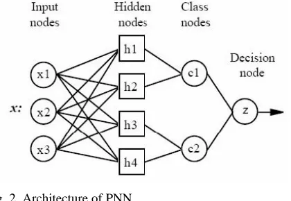
[image:2.612.324.534.547.692.2]Many classifiers have been used for ECG classifications in the past [1][4][5].The Probabilistic neural network is a feed forward neural network that implements a Bayesian decision strategy for classifying input vectors. The basic architecture appears as in fig.2.
Fig. 2. Architecture of PNN
pattern node. There is one pattern unit for each exemplar in the training set .The weight vector for each pattern unit is a copy of the corresponding exemplar, and is also normalized. Moreover, training is accomplished by adding pattern units with the appropriate weight vectors in place.
In the pattern units, we take the dot product of the input vector and the weight vector, as is typically done in feed-forward networks. We then use a nonlinear output function. Here we used the Gaussian function. In the category layer or the class layer, summing the outputs of all the pattern units belonging to a class is done. we have in effect computed the posteriori probability distribution function for that class, evaluated at the input point. Classification is done in the decision node. The output is the class which gives the highest response.
C. Feature Extraction.
The immediate step after decomposition of the signal is feature extraction from the sub-bands. The features are extracted for all bands and sub-bands.
Altogether twenty features were extracted from a single QRS complex. Feature sets are derived by combining different features. These feature sets are given as input to the classifier and trained. With testing sets, the accuracy was cross checked.
Following are the features calculated from bands and sub bands.
σR – variance of the autocorrelation function. Q – relative amplitude.
P – power of the decomposed signal.
Following two features are common for entire QRS Complex.
σx – variance of the original signal. RR – Successive RR interval
1) Power of the sub-bands:
Signal variance is calculated using the formula P= 1/N ∑{x2(n)}, ∑ runs from 1 to N. N=number of samples.
x(n)=signal.
The signal variance in a sub band represents the average AC power in that band.
2) Variance of the autocorrelation function:
The autocorrelation function can be used as a measure of similarity or coherence between a signal
x(n) and its shifted version. If x(n) is of length N, its autocorrelation function is expressed as
R(l) = ∑ x(n) x(n-1)
where l is the time shift index, i=l, k=0 for l >=0, and i=0, k=l for l<0.
The variance of the autocorrelation, σ R, represents the averaged AC power of the autocorrelation function, which measures the coherence of the decomposed signal in each sub band.
3) Relative amplitude of the signal:
Relative amplitude of the signal x(n) is found by the formula
Q= min(x(n))/ max(x(n));
Q is found for all the sub-bands of the signal. Including this, the three features discussed till now are common for all the sub-bands.
4) RR interval of the signal:
Certain ECG arrhythmia, such as APB and PVC, are related with premature heart beats that provide shorter RR intervals than other types of ECG signals. Successive RR interval is found for every QRS complex. Successive means RR interval in seconds between the current R peak and the next R peak.
D. Normalization
Since the features are to be fed into a neural network it is normalized and the hyperbolic tangent sigmoid function is used for the normalization. After normalization the features lies in the range of -1 to +1.
x1ij = tansig(xij – mean(xj)/(variance (xj)));
xij = jth component of ith feature vector.
x1ij = normalized feature vector.
E. Experimental Procedure
The feature set formation discussed in Section C is ordered as in Table.1.
execution time and didn’t make significant contribution to accuracy. There were other combinations of features also tested as you can see in Table.1.
3. RESULTS
Training for all the six types of beats are given to the neural networks. Few type of records have very less number of QRS complex and they demand more training. Few records have good number of QRS complex and in such cases lesser amount of training is enough.19,517 complex are extracted and 80% of it are used for training. Maximum accuracy of 85% is achieved by using feature set 6. Table.2 shows the record selection.
The feature sets for all the records in the Table.2 are created and given as input for the PNN. The Accuracies of classifier for all the feature sets are compared. After deploying classifiers under different spread, feature set six performs well and classifies the beats very well when compared, which means it is not necessary for two stage full binary decomposition of the signal as two stage two band decomposition performs better.
Spread Selection
Spread is an important parameter for many classifiers Like PNN. Classification of types of signals may vary with different spread values. Challenge lies in selecting spread values for a particular classification problem, the best and common method for spread selection is just by training all the samples and testing the same or few from what was trained.
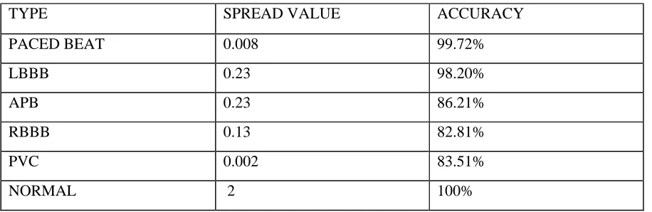
The output for test cases should be of maximum accuracy. Spread values from 0.0 are increased by the order of 0.05 and a region is spotted out where accuracy is very high. From this region an optimal spread is found and given for classification. Table.3 show accuracy for different spread values. Here 80% of samples are trained and 20% of the samples are tested. The statistic employed to evaluate the performance of our proposed method is defined as follows
Accuracy = No of correct classified beats / No of total beats
From Table.3 it is seen that the accuracy of correct classification is greater for spread values 0.23 and less. For values less than 0.23 the accuracy values for most of the feature sets are same as for 0.23. Even though each and every beat is having its own spread value, the spread value of 0.23 gives a reasonable accuracy of over 80% for
all beat types. Hence the selection of spread as 0.23 is justified.
4. CONCLUSIONS
We have proposed a classification scheme for ECG signals based on wavelet transform and PNN classifier. We found that two stage two band decomposition is sufficient and better than full stage full binary decomposition. The optimal feature set achieves a good accuracy of 84.35 %. On varying the spread values we got a highest accuracy of 99.72% for Paced beat. The total number of features required to attain this accuracy is only 11. This is substantially better than other methods. Also the RR component plays an important role to discriminate high risk PVC and APB related heart diseases.
REFRENCES:
[1] Kuan-To Chou and Sung-Nien Yu.’
Categorizing Heartbeats by Independent Component Analysis and Support Vector Machines’, Eighth International Conference on Intelligent Systems Design and Applications [2] Tanveer Syeda-Mahmood, David Beymer, and
Fei Wang.’ Shape-based Matching of ECG Recordings’, Proceedings of the 29th Annual International Conference of the IEEE EMBS Cité Internationale, Lyon, France August 23-26, 2007.
[3] Ying-Hsiang Chen and Sung-Nien Yu.’ Comparison of Different Wavelet Sub band Features in the Classification of ECG Beats Using Probabilistic Neural Network’, proceedings of the 28th IEEE EMBS Annual International Conference New York City, USA, Aug 30-Sept 3, 2006
[4] Guangchen Liu and Mei Song.’ Application of a BP Network Based on PCA in ECG Diagnosis of the LVH’
[5] Sung-Nien Yu1 and Kuan-To Chou.’ Combining Independent Component Analysis and Back propagation Neural Network for ECG Beat Classification’, Proceedings of the 28th IEEE EMBS Annual International Conference New York City, USA, Aug 30-Sept 3, 2006 [6] Zhi-Dong Zhzo and Yu-Quan Chen.’ A NEW
Par ent
Feat ure
F1 F2 F3 F4 F5 F6 F7 F8 F9 F10 F11 F12 F13 F14 F15
x[n] σx X X X X X X X X X X X X X X X
σR X X X X
L P X X X X
Q X X X X
σR X X X X X X
H P X X X X X X
Q X X X X X X
σR X X X X X X X X X X
P X X X X X X X X X X
LL Q X X X X X X X X X X
σR X X X X X X X X X X
LH
P X X X X X X X X X X
Q X X X X X X X X X X
σR X X X X X X X X
P X X X X X X X X
HL Q X X X X X X X X
σR X X X X X X X X
P X X X X X X X X
HH Q X X X X X X X X
RRI X X X X X X X X X
N 14 11 11 11 11 11 10 19 7 7 7 20 8 8 8
Table.1 Different Feature Sets Used To Classify QRS Complexes. Σx Is Variance Of Original Signal. Σr Is The Variance Of Auto Correlation Function. P Is The Power Of Decomposed Band. Q Is The Relative Morphological Characteristic. RRI Is The RR Interval And N Is The Number Of Features Included In Corresponding
Record number
Type of complex
Class Training percentage
Total number of complex in the signal
Total Training complex
Total Testing complex
Accuracy for F 6
107 PB 1 80 2077 1662 415
86.03%
217 PB 1 80 1541 1233 308
207 L 2 70 1456 1019 437
98.80%
214 L 2 70 1400 980 420
209 A 3 95 382 362 20
86.31%
232 A 3 95 1381 1311 70
124 R 4 80 1530 1224 306
72.47%
212 R 4 80 1824 1459 365
231 R 4 80 1253 1002 251
118 R 4 80 2165 1732 433
200 PVC 5 95 825 808 17 70.83%
221 PVC 5 95 395 375 20
113 N 6 80 1788 1430 358
91.65%
220 N 6 80 1500 1200 300
[image:7.612.87.548.71.488.2]TOTAL NUMBER OF COMPLEX 19517 15797 3720
84.35%
Table 2. Selection Of Records For Training And Testing.
TYPE SPREAD VALUE ACCURACY
PACED BEAT 0.008 99.72%
LBBB 0.23 98.20%
APB 0.23 86.21%
RBBB 0.13 82.81%
PVC 0.002 83.51%
NORMAL 2 100%
[image:7.612.84.542.527.676.2]