Computer Science Dissertations Department of Computer Science
12-14-2017
Towards Data-driven Simulation Modeling for
Mobile Agent-based Systems
Nicholas Aiden Keller
Follow this and additional works at:https://scholarworks.gsu.edu/cs_diss
This Dissertation is brought to you for free and open access by the Department of Computer Science at ScholarWorks @ Georgia State University. It has been accepted for inclusion in Computer Science Dissertations by an authorized administrator of ScholarWorks @ Georgia State University. For more information, please [email protected].
Recommended Citation
Keller, Nicholas Aiden, "Towards Data-driven Simulation Modeling for Mobile Agent-based Systems." Dissertation, Georgia State University, 2017.
SYSTEMS
by
NICHOLAS KELLER
Under the Direction of Xiaolin Hu, PhD
ABSTRACT
Simulation modeling provides insight into how dynamic systems work. Current
simulation modeling approaches are primarily knowledge-driven, which involves a process of
converting expert knowledge into models and simulating them to understand more about the
system. Knowledge-driven models are useful for exploring the dynamics of systems, but are
handcrafted which means that they are expensive to develop and reflect the bias and limited
knowledge of their creators. To address limitations of knowledge-driven simulation modeling,
this dissertation develops a framework towards data-driven simulation modeling that discovers
simulation models in an automated way based on data or behavior patterns extracted from
discovered that replicate the desired behavior. Each of these models can be thought of as a
hypothesis about how the real system generates the observed behavior. This framework was
developed based on the application of mobile agent-based systems. The developed framework is
composed of three components: 1) model space specification; 2) search method; and 3)
framework measurement metrics. The model space specification provides a formal specification
for the general model structure from which various models can be generated. The search method
is used to efficiently search the model space for candidate models that exhibit desired behavior.
The five framework measurement metrics: flexibility, comprehensibility, controllability,
compossability, and robustness, are developed to evaluate the overall framework. Furthermore,
to incorporate knowledge into the data-driven simulation modeling framework, a method was
developed that uses System Entity Structures (SESs) to specify incomplete knowledge to be used
by the model search process. This is significant because knowledge-driven modeling requires a
complete understanding of a system before it can be modeled, whereas the framework can find a
model with incomplete knowledge. The developed framework has been applied to mobile
agent-based systems and the results demonstrate that it is possible to discover a variety of interesting
models using the framework.
SYSTEMS
by
NICHOLAS KELLER
A Dissertation Submitted in Partial Fulfillment of the Requirements for the Degree of
Doctor of Philosophy
in the College of Arts and Sciences
Georgia State University
Copyright by Nicholas Aiden Keller
SYSTEMS
by
NICHOLAS KELLER
Committee Chair: Xiaolin Hu
Committee: Robert Harrison
Xin Qi
Ying Zhu
Electronic Version Approved:
Office of Graduate Studies
College of Arts and Sciences
Georgia State University
DEDICATION
ACKNOWLEDGEMENTS
I would like to thank my advisor Dr. Xiaolin Hu for teaching me how to conduct and
document my research. I would also like to thank my Committee members Dr. Robert Harrison,
Dr. Xin Qi, and Dr. Ying Zhu. Finally, I would like to thank the Computer Science Department
TABLE OF CONTENTS
ACKNOWLEDGEMENTS ... V
LIST OF TABLES ... X
LIST OF FIGURES ... XII
1 INTRODUCTION ... 1
1.1 Introduction to Modeling ... 1
1.2 Computer Modeling ... 1
1.3 Data-Driven Modeling ... 3
1.4 Knowledge-Driven Modeling ... 4
1.5 Current Limitations of Knowledge-Driven Modeling ... 6
1.6 Agent-Based Modeling ... 8
1.7 Outline of Framework ... 9
1.8 Incorporating Incomplete Knowledge Into the Framework Through System Entity Structures (SESs) ... 12
1.9 Organization ... 13
2 REVIEW OF LITERATURE... 14
2.1 Introduction ... 14
2.2 Mobile Agent Modeling ... 15
2.3 Knowledge-Driven Mobile Agent Modeling ... 16
2.5 Hybrid Mobile Agent Modeling ... 17
3 SIMULATION MODELING FRAMEWORK... 19
3.1 From Knowledge-Driven Simulation Modeling to Data-Driven Simulation Modeling 19 3.2 Framework Overview ... 22
3.3 Model Space Specification ... 24
3.3.1 Agents ... 25
3.3.2 Behavior Groups ... 27
3.3.3 Behaviors ... 28
3.3.4 Simulation of a Model... 32
3.4 Model Space Search ... 33
3.4.1 Genetic Algorithm ... 34
3.4.2 Simplification ... 35
3.4.3 Fitness functions ... 36
3.4.4 Composite Fitness Functions ... 37
3.5 Framework Evaluation Metrics ... 39
3.5.1 Flexibility ... 39
3.5.2 Comprehensibility and Controllability ... 40
3.5.3 Composability ... 40
4 EXPERIMENTAL RESULTS AND ANALYSIS FOR DATA DRIVEN
SIMULATION MODELING ... 43
4.1 Experimental Setup ... 43
4.1.1 Fitness Metrics Used ... 46
4.2 Interpreting Discovered Models: Comprehensibility, Sensitivity Analysis, and Robustness ... 51
4.2.1 Snake Shape Model ... 52
4.2.2 Snake Shape with Obstacle Avoidance ... 60
4.2.3 Hollow Circle Shape Model ... 67
4.3 Controllability and compossability ... 70
4.3.1 Adding Personal Space to Snake Model ... 70
4.3.2 Modifying Boids Model ... 73
5 INCORPORATING KNOWLEDGE INTO DATA-DRIVEN MODELING THROUGH THE USE OF SYSTEM ENTITY STRUCTURES (SES'S) ... 76
5.1 Introduction to System Entity Structures (SESs)... 76
5.2 Using SES to Discover Mobile Agent Models ... 78
5.3 SES Applied to Lane Formation ... 81
5.3.1 Experimental Setup ... 81
5.3.2 Analyzing the Discovered Lane Formation Model ... 86
LIST OF TABLES
Table 3.1 Property combination functions for: position, angle, and speed ... 30
Table 3.2 Key framework variables: entity categories/types, extractable properties, and filter properties... 32
Table 4.1 Experimental design and analysis overview ... 46
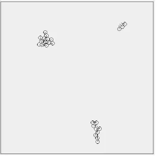
Table 4.2 Simplified snake model ... 55
Table 4.3 Snake shape model combination method sensitivity analysis ... 58
Table 4.4 Snake shape model's first behavior's filter sensitivity analysis with respect to snake shape fitness metric ... 59
Table 4.5 Snake shape with obstacle avoidance model before polishing and analysis ... 62
Table 4.6 Snake shape with obstacle avoidance model after polishing (but before simplification) ... 62
Table 4.7 Snake shape with obstacle avoidance model after polishing and simplification ... 63
Table 4.8 Snake shape with obstacle avoidance model's 3rd behavior's sensitivity analysis with respect to touches obstacle fitness metric ... 65
Table 4.9 Snake shape with obstacle avoidance model's 3rd behavior's combination method analysis ... 65
Table 4.10 Hollow circle model... 68
Table 4.11 Hollow circle model's 1st behavior's combination method sensitivity analysis ... 69
Table 4.12 Snake shape model with personal space preservation ... 71
Table 4.13 Handcrafted boids model ... 74
Table 5.1 Behavior restrictions ... 85
Table 5.3 Lane formation model's 1st behavior's filter range analysis for travel time metric ... 88
Table 5.4 Lane formation model's 2nd behavior's 1st filter's range analysis for travel time metric
... 89
Table 5.5 Lane formation model's 2nd behavior's 1st filter's range analysis for hallway density
metric ... 89
Table 5.6 Lane formation model combination method analysis ... 90
LIST OF FIGURES
Figure 1-1 Framework ... 12
Figure 3-1 Knowledge-driven simulation modeling process ... 19
Figure 3-2 The framework modeling process ... 21
Figure 3-3 Extending the framework modeling process ... 22
Figure 3-4 Data-driven simulation modeling framework components ... 23
Figure 3-5 An agent's field of view determines what entities (agents, obstacles, and zones) it can see ... 27
Figure 3-6 Example of behavior that turns the observing agent 10 degrees away from nearby agents ... 30
Figure 3-7 Sense-think-act cycle controlling an agent's heading ... 33
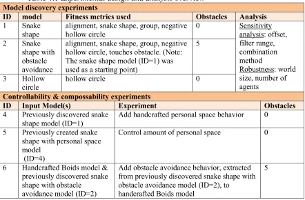
Figure 4-1 Snake shape model ... 53
Figure 4-2 Snake shape model with behavior filter removed resulting in bad behavior ... 54
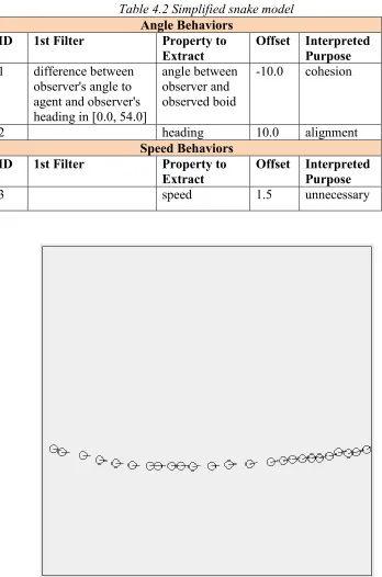
Figure 4-3 Snake model with unnecessary speed behavior removed ... 55
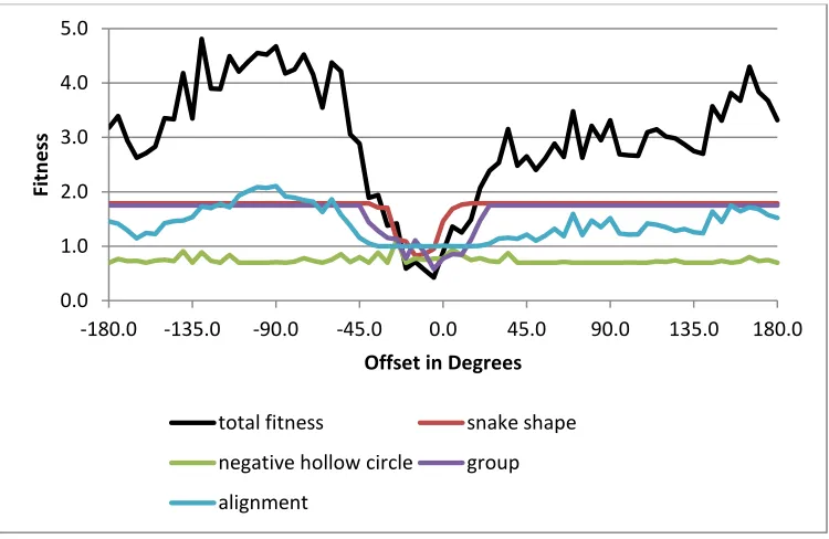
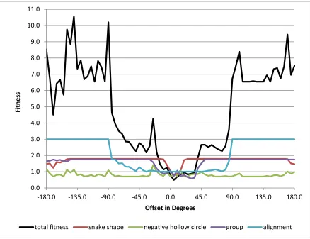
Figure 4-4 Snake shape model's 1st behavior's offset sensitivity analysis ... 56
Figure 4-5 Snake shape model's 2nd behavior's offset sensitivity analysis ... 57
Figure 4-6 Snake shape model's 2nd angle behavior's combination method is set to "closest" resulting in bad behavior ... 58
Figure 4-7 Snake shape model's world size robustness analysis ... 60
Figure 4-8 Snake shape with obstacle avoidance model ... 61
Figure 4-9 Snake shape with obstacle avoidance model's 3rd behavior's offset analysis... 64
Figure 4-11 Snake shape with obstacle avoidance model's number of obstacles robustness
analysis ... 67
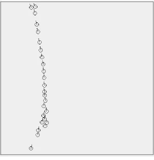
Figure 4-12 Hollow circle model ... 68
Figure 4-13 Hollow circle model's 1st behavior's offset sensitivity analysis ... 69
Figure 4-14 Snake shape model with personal space; personal space distance = 24, world size = 800x800... 72
Figure 4-15 Snake shape model with personal space; personal space distance =48, world size 800x800... 73
Figure 4-16 Handcrafted boids model ... 74
Figure 4-17 Handcrafted boids model with added obstacle avoidance behavior taken from the discovered snake shape with obstacle avoidance model... 75
Figure 5-1 Converting car SES into car PES ... 77
Figure 5-2 Generating a model from a SES and entity model database ... 78
Figure 5-3 Progressing from general framework SES to model space search PES ... 80
Figure 5-4 Hallway zones used in lane formation model search ... 82
Figure 5-5 Lane formation model simulation. Panel A shows the zone and subzones used in the hallway density metric, which is hidden in panels B through F ... 86
Figure 5-6 Lane formation model's 1st behavior's offset sensitivity analysis ... 91
Figure 5-7 Lane formation model's 2nd behavior's offset sensitivity analysis ... 91
Figure 5-8 Lane formation model's 3rd behavior's offset sensitivity analysis ... 92
1 INTRODUCTION
1.1 Introduction to Modeling
People model things all the time whether they realize it or not. In conversation we use a
model of the other person to leave out details that we think they are either uninterested in our
already know. Sometimes our internal models are wrong, such as when a computer science PhD
student teaches their first class and doesn't realize that the class hasn't fully learned Java syntax
yet. People revise their models based on experience that is either direct; the look of confusion on
students' faces, or vicariously such as through books.
A model is an abstract representation of some aspect of the real world. All models are
wrong, because they aren't a perfect representation of the real world, but some are useful.
Creating a useful model requires determining what to leave out of a model and what to include
based on its purpose. When deciding whether to keep lifesavings as cash or in stocks it is useful
to know that inflation will overtime eat away at the purchasing power of cash. When day trading
stock at a hedge fund a much more detailed model of inflation and its relationship to interest
rates is needed. The more detailed a model the more expensive it is to create and use. For the
hedge fund this extra cost is worth it, but for the individual investor it is a waste. The goal of all
models is to provide some knowledge about the real system by simplifying it.
1.2 Computer Modeling
Although people are natural modelers they frequently aren't particularly good modelers.
Many systems are well understood by experts; however, the dynamics of the system are too
complicated to understand without the help of computers. One such system is supply chain
predicting without stock and flow computer models [22]. Computers make it possible to build,
analyze, and use complex models.
Computers, which don't have the same processing limitations as people, can simulate the
interaction between multiple components. For example, a model of a crowd can model the
decision process of each person [21]. A computer model of child maltreatment can take into
account the sharing of resources between families in a heterogeneous community [23]. A stock
and flow model of the housing market can capture the complexity of the system in a way an
un-aided human mind never could.
The data processing abilities of computers also makes it possible to analyze and use
models in ways that aren't possible with peoples' internal models. For example, language
translation models make language translation faster and cheaper than using human translators;
although it is not as accurate yet. The model of the world that self-driving cars create and use has
the potential to substantially reduce accidents, because computers can react faster than humans to
possible collisions and can see more through better sensors. Even when a computer model is easy
to understand and interpret, which is not necessarily the case in the language translation and
self-driving car examples, computers lets us run thousands of experiments.
Computer modeling has two broad applications: 1) making predictions, and 2) testing
hypotheses about how real systems work. Some models like those of weather and image
recognition are focused on prediction, whereas others like the Boids model of flocking [3] are
focused on hypothesis testing. The Boids model [3] hypothesizes that just three behaviors lead to
bird flocking behavior; alignment, collision avoidance, and cohesion. This hypothesis is
supported when the boids model generated flocking behavior similar to that observed in nature.
based on some theory and then, after it is validated by comparing its behavior to the real system,
it is used to make some predictions about the system. Computer modeling can be approached
from a data-driven or knowledge-driven perspective as will be discussed next.
1.3 Data-Driven Modeling
Data-driven modeling is used to refer modeling techniques that use data to build models.
Data-driven modeling also goes by the names artificial intelligence or machine learning. Some
examples of big data are: data collected from Tesla's cars while they are driven [31], labeled
images taken from the internet [24], and United Nations (U.N.) meeting translations [25].
Data-driven modeling makes creating large models fast and relatively inexpensive. It is a lot easier to
build a language translation program using data, then to hand code every quirk of a language.
Furthermore, it may not even be possible to handcraft a language translation program, because
the language may evolve faster than you can encode a model for it. The goal of data-driven
modeling is primarily prediction.
The primary disadvantage of data-driven modeling is that it results in incomprehensible
models, which makes them difficult to validate. Although on a technical level a model created
using data can be read, on a conceptual level it is opaque; it's just a jumble of numbers that hides
its structure. In an admission of this problem, DARPA recently asked for proposals on how to
assure the correctness of driven models [26]. The only way to check the correctness of
data-driven models is through tests with sample data. Typically data used to train a model is split into
data used for training and data used for testing the trained model for accuracy. Testing a model
on data used to train it can lead to a model looking better than it is because of overfitting the
training data. Unlike code, data-driven models can't be examined to see if they are correct. This
against. For example, a computer vision program used to recognize street signs was trained to
ignore a stop sign with a sticky note on it [27]. It is impossible to test for all kinds of malicious
information that might be surreptitiously embedded in a data-driven model. An alternative to
data-driven modeling is knowledge-driven modeling that gets rid of the opaqueness problem of
data-driven models, but sacrifices the ability to quickly build large complex models using data.
1.4 Knowledge-Driven Modeling
Knowledge-driven modeling is used to refer to modeling techniques that use knowledge
from experts to build models. Unlike data-driven models, these models are handcrafted. A given
model is made up of components taken from theory, which results in comprehensible models.
For example, theories of crowd behavior that rely on the individual decisions of people in the
crowd are best represented with agent-based models, where each person is modeled individually
[21]. Other theories see people evacuating a building as flows of people in a macro level network
model where nodes are rooms and edges represent the flow capacity of doors and hallways [28].
Although different, it is possible that these two models can both be correct at their own level of
abstraction. Computer modeling can help formalize a theory, test it, and work out its
implications. If a system is well understood (or we think it is) then knowledge-driven modeling
is a good fit.
Unlike data-driven models knowledge-driven models can be simulated. For this reason
knowledge-driven modeling is sometimes also called simulation modeling. A simulation is a
story about how a system works and is similar, but distinct from prediction. Simulation is about
the journey not just the destination; how a system reaches an end state is just as important as
such as stock market trading bots [29]. Simulation models are built out of components inspired
by theories about how a system works.
At a mechanical level simulation models are rules about how a system state changes from
one time to another. Let us say we want to model the trajectory of a soccer ball for 10 seconds
just after its been kicked into the air. A discrete time model would split up the trajectory into
equal time segments; say 1 second per segment. The modeling problem then becomes predicting
what the location of the ball will be 1 second in the future based on the soccer ball's speed, the
effect of gravity, wind resistance, and the possibility that it will hit people or the ground. Since
the real world doesn't operate in 1 second increments the model will be inaccurate. A collision
that might occur at 1.1 seconds will instead be represented as occurring at either 1 or 2 seconds.
To improve accuracy the time segments can be made smaller, but this increases the
computational cost of running the model.
Continuing the soccer ball example, we can improve model accuracy while potentially
speeding up computation by using a continuous time model that calculates the next event. In this
example, the soccer ball is flying through the air and the next possible events are that it hits the
ground or hits another player (to improve efficiency the rare event of a goal is intentionally not
modeled). If the next event is say 5 seconds in the future then only 1 event needs to be calculated
instead of 5 separate discrete time states. The ball of course could have more than 10 events over
10 seconds (for example, the ball bouncing), but this model would still be better than the discrete
time model, because it would simulate those events. The only down side is that calculating the
next event can be very time consuming; each player has to be tested to see if and when it will hit
the soccer ball and the earliest event is chosen. Sometimes the cost of calculating the next event
Discrete time models can be made as accurate as needed by decreasing the time
increment and are easier to develop than continuous time models. It is for this reason that one
modeling technique is to develop a discrete time model and once its value is proven it can be
converted (with great effort) to a continuous time model to improve efficiency. With this in mind
the model used in this dissertation is a discrete time model.
1.5 Current Limitations of Knowledge-Driven Modeling
A system can be represented by multiple simulation models that each approaches the
system from a different level of abstraction; as in the crowd behavior example mentioned in the
previous section. What distinguishes simulation modeling from other modeling techniques is that
it uses abstractions that relate to some theory about a system. One issue in simulation modeling
is that the process of converting theory into a simulation model is ad-hoc. However, the real
elephant in the room of simulation modeling is that a simulation model is only as strong as the
theory it is built upon; what if that theory is flawed or incomplete?
A simulation model that replicates the behavior of a real world system is not necessarily
an accurate representation of it. If a model reproduces observed behavior, then this lends support
to the theories behind the model, but doesn't prove those theories are correct. A model whose
purpose is purely predictive, not a simulation model, is evaluated based on the accuracy of its
predictions. A simulation model in addition to its predictive accuracy is also evaluated by how
accurately it represents the real system. If the real system is opaque, and almost all real systems
are at least partially unobservable, then the model's predictive accuracy is used to evaluate a
simulation model's structure. However, this method cannot fully validate a model because a
model can be predictive without being structured like the real system. It is not without merit
this reason that a simulation model can be thought of as an embodied hypothesis about how a
system works and not necessarily an actual abstraction of the real system.
If a simulation model perfectly replicates the behavior of the real system, than there is a
high likelihood that its structure reflects the structure of the underlying system; however, there is
usually ambiguity when comparing model to system behavior. When modeling a system the goal
is to replicate the "behavior" of the system and not the exact time series states of the system.
Even if a model perfectly represented a system small variations in initial conditions would lead it
to vary from the real system slightly. Therefore, measurements of behavior are subjective even
when quantitative functions are used. For example, the path of a hurricane can be measured
quantitatively both in the real system and a model, but what level of difference is acceptable?
This can partially be answered by simply preferring models with better predictions, but when is a
model as good as it can be? In many domains it is even a challenge to quantitatively measure
behavior. An early model of bird blocking, called Boids [3], presented pictures of simulated bird
flocks as a form of evidence.
A simulation model that reproduces real system behavior provides some knowledge
about that system, but should not be thought of as the final say in how a system works. However,
the painstaking process by which simulation models are created by hand results in too few
models of a system. Furthermore, since models are generated by hand they can only test theories
and not generate new ones, because they reflect the preconceptions of their creators, which
results in biased models. The solution is to generate human readable (comprehensible) models
automatically. These models would be easy to interpret like knowledge driven models, but would
not have the bias inherent in the creation of knowledge driven models. The framework presented
1.6 Agent-Based Modeling
The framework presented in this dissertation uses agent-based modeling, which is a type
of knowledge-driven modeling. In an agent-based model each entity (agent) in a system is
modeled separately. For example, in crowd model each person is modeled individually or in a
model of traffic each car would be modeled separately. Each agent can only observe part of the
environment and neighboring agents. For example, a person in a crowd can only observe their
neighbors and nearby obstacles. Although each agent acts separately based on local knowledge a
collective behavior emerges. Agents act based on what they see their neighbors doing, so
information and behavior can "ripple" through an environment. For example, one car randomly
slows down, which causes the car behind it to slow down and the car behind that to slow down as
well and so on until a traffic jam results; this has been demonstrated with real cars on a circular
closed course [30]. Agents don't have to take up physical space. For example, they could be
people connected through a social network or companies in an economy connected through
supply chains.
Mobile agent models represent a large subset of agent-based models and is the type of
model studied using the presented framework. A mobile agent model is one were agents move in
a space representative of a real world environment. The space can be 2D as is the case with
people in a crowd. Or 3D as is the case with simulated flocks of birds and fish. Or even 1D in a
model of a 1 lane road. In a mobile agent model, agents can view nearby agents and
environmental features (walls in a room for example). A simple model of vision is that
everything within some distance to the agent is visible. For mobile agent models of living things
a vision model based on a field of view is more realistic. However, although people have a
to model their field of view as being 360° or at least greater than their physiological field of
view. The framework focuses on mobile agent modeling, although it can be generalized to other
types of modeling, because it is a significant area of research.
1.7 Outline of Framework
This dissertation proposes a framework for using data to automatically generate
simulation models, so that models can be created faster and with less bias than current
handcrafting simulation modeling methodologies. A simulation model is a hypothesis about how
a system works, so a framework for generating these hypotheses with less bias is a significant
contribution. Existing data-driven modeling methods are focused on prediction and result in
black box models that provide no insight into how systems produce behavior unlike the proposed
method. This is the first framework for discovering simulation model structure automatically
using data. To demonstrate the utility of the proposed framework it was applied to the mobile
agent domain, although the framework is general enough to be applied to any domain. The major
contributions of the dissertation are to the mobile agent domain and modeling methods more
generally.
The approach is to define a very large space of possible models of real systems, then
search through this space for a model which generates a real systems behavior. Since models can
be discovered automatically, multiple models can be discovered, which opens up a whole new
way of studying systems. Multiple models means multiple hypothesis about how a real system
works, whereas existing modeling techniques have limited themselves to only one hand crafted
model, hypothesis, at a time. Under this framework the work of a modeler shifts from creating a
model from scratch to the task of defining the model space and creating behavior description
specific model, which both reduces modeler bias and has the potential to speed up model
development.
The three broad research challenges were model space specification, model search, and
the analysis of discovered models. Unlike black-box modeling the model space must contain
comprehensible models whose behavior is easily understood by an examination of the model.
The challenge is creating a model space that contains an interesting variety of models, but
remains comprehensible. The model space is searched using an application of the genetic
algorithm, but as will be discussed later there are issues unique to the framework that must be
addressed. The model space search requires a model evaluation algorithm (fitness function)
which requires a precise definition of the behavior being looked for. The fitness of a model is
measured as the difference between the behaviors a model generates and the idealized behavior.
As discussed in 1.5 Current Limitations of Knowledge-Driven Modeling defining behavior
quantitatively is challenging. The model that is discovered by the search process must be cleaned
up to remove non-essential model components and thoroughly analyzed to yield insights into the
system. Cleaning up a discovered model is a completely new modeling step that isn't required for
data-driven models that are purely predictive or knowledge driven models that are
comprehensible by virtue of being handcrafted.
The framework was applied to the mobile agent domain, but is not limited to this domain.
The mobile agent modeling domain was chosen because of its broad applicability. Mobile agent
modeling has been applied to building evacuations [3], understanding swarms of animals [1], and
swarm robotics [4]. The framework uses agent-based modeling to study mobile agents
To evaluate how well the framework was applied to the mobile agent domain we
developed five measurement metrics: 1) flexibility, 2) comprehensibility, 3) controllability, 4)
composability, and 5) robustness. If the framework were applied to another domain, than these
measurement metrics could be used to evaluate this application. The framework is flexible if it
can be used to discover a variety of non-trivial mobile agent models. Discovered models that are
easily interpreted are comprehensible. A model is controllable if a modeler can comprehend it
and then modify it to achieve predictable changes in behavior. Controllability is important
because it demonstrates comprehensibility, but it is also of practical value in and of itself. For
example, a model of pedestrians might be modified to change the personal space between people
to reflect different culturally specific expectations of personal space. This would allow a model
trained on one set of historical data to be used in another context. This sort of out of context
model re-use is impossible with typical data-driven models. In the framework, models are
composed of competing behaviors; cohesion and collision avoidance for example.
Compossability means that discovered or hand crafted behaviors can be predictably combined to
create new models. Compossability is important because it makes the framework more useful by
allowing modelers to mix and match already discovered or known (hand crafted) behaviors. It
makes the creation of a library of useful behaviors possible. Finally, models must be robust or
they aren't useful. Robust models are one that aren't highly sensitive to specific conditions like
the number of people, the size of the environment, or the number of obstacles in the
environment. These metrics should be used to evaluate the framework's application to the mobile
agent domain.
An outline of the framework is given in figure 1.1 below. The search step requires a
step which can take many hours a candidate model is output. The candidate model is "fit," but is
still considered a candidate because it is a hypothesis about how the system works. The
suitability of a particular framework implementation is determined by how well it satisfies the
five measurement metrics.
Figure 1-1 Framework
1.8 Incorporating Incomplete Knowledge Into the Framework Through System Entity
Structures (SESs)
The framework uses System Entity Structures (SESs) to rigorously incorporate
incomplete knowledge of mobile agent behavior. One of the earliest publications on SES is from
1990 [2]; however, its application in this framework is novel. Typically SES is used to represent
different system structures, but in the framework it is used to represent incomplete knowledge of
a system. Whereas knowledge driven modeling forces a modeler to completely understand a
system to model it, the framework uses SES to allow the modeling of partially understood
systems. Most systems are incompletely understood, so this technique can greatly expand the
number of systems that can be represented by comprehensible models that provide insight into
SESs are tree like structures that show all the different possible decompositions of a
system model into its component entities. For example, a SES could be used to model a car. The
car SES would show all the different possible cars that could be made from different
components, such as different models of engine. An example of a car SES is given in figure 5-1
in chapter 5. A SES is pruned to create a Pruned Entity Structure (PES) which represents specific
entities that are used to create a model. The last step is convert the PES into a model of the
system that can be simulated.
In the case of the mobile agent framework, the entities are behavior restrictions. A
behavior restriction defines a set of behaviors that satisfy those restrictions. The restrictions
represent knowledge that the modeler wants to incorporate into the search process. When a
behavior is unrestricted it means that the modeler has no knowledge about the purpose of a
behavior (even whether it is needed in the first place). For example, let us say that a modeler is
modeling a situation where child agents follow a teacher agent on a field trip. The modeler
knows that at least one of the child agent's behaviors must be restricted to observe the teacher
agent. Even though the modeler doesn't completely understand the system they can still provide
what they do know. A PES in the framework represents a set of restricted and unrestricted
behaviors. The PES is converted into a model by randomly selecting behaviors from the set of
behaviors defined by the behavior restrictions.
1.9 Organization
The rest of this dissertation is organized as follows. The review of literature in chapter 2
places my research within the modeling and mobile agent domains. Chapter 3 presents the details
of the framework including the model space specification, search method, and framework
framework. Finally, chapter 5 discusses how the framework defined in chapter 3 is extended to
incorporate incomplete knowledge through the use of System Entity Structures (SESs). Chapter
5 also includes an experimental results section where the SES extended framework is used to
discover a lane formation model.
2 REVIEW OF LITERATURE
2.1 Introduction
This dissertation makes contributions to the mobile agent modeling domain. Mobile agent
models fall within one of three major categories; knowledge-driven, data-driven, and hybrid.
Knowledge-driven models are handcrafted by a modeler to reflect their understanding of the
system. A knowledge-driven model is the formalization of theory into a program that allows for
simulation, therefore these models are easy to understand. Data-driven models are derived from
data in an automatic or semi-automatic manner. Data-driven models are focused on prediction
and unlike knowledge-driven models, they do not provide knowledge about the underlying
causes of system dynamics. Hybrid models combine an upper layer that determines agents'
overall movement objectives (data-driven) with a microscopic lower level model which controls
agent collision dynamics (knowledge-driven).
The proposed framework is unique in that it combines features from data-driven and
knowledge-driven mobile agent modeling. Like data-driven modeling the framework
automatically discovers models using data (or a quantitative description of the desired behavior).
However, unlike data-driven modeling the proposed framework results in models that are
comprehensible and provide insight into the underlying causes of mobile agent behavior. Like
driven modeling the framework produces readable models, but unlike
framework represents the first step in a new mobile agent modeling category that I propose
should be called "data-driven simulation modeling."
2.2 Mobile Agent Modeling
A system can be simulated using a mobile agent-based model if it contains many similar
agents, such as people, that move around in a shared environment, act autonomously, and only
have local knowledge (and possibly global knowledge about the environment; like a familiar
building's layout). Groups of animals whether they be flocks of birds, herds of cattle, or schools
of fish can be studied using mobile agent modeling [3] [18]. Mobile agent-based modeling can
also be used to study how groups of people move through a building [4], crowd [5], or in traffic
[6]. Swarms of robots are an increasingly important area of research [7].
Studies of animal systems are mainly focused on theoretical research, whereas studies of
human mobile-agent systems tend to have a more practical focus. Models of car traffic can be
used to design road systems and to predict congestion on roads [19] [20]. Models of pedestrians
can be used to design stadiums for large numbers of people under regular conditions and to
safely evacuate people in emergencies [4]. Models can also be used to understand how people
move through an existing space, so that this space can be modified to improve its efficiency [21].
There are three broad mobile agent modeling approaches; knowledge-driven, data-driven,
and hybrid. Knowledge-driven models are handcrafted models that implement some theory about
how a system works. Data-driven models use data to automatically generate a mobile agent
model. Hybrid models have parts that are handcrafted and parts that are generated from data.
Each of these mobile agent modeling methods has disadvantages relative to the proposed
2.3 Knowledge-Driven Mobile Agent Modeling
Knowledge-driven mobile agent modeling results in very readable models. Experts can
examine a model and decide whether they agree with how it abstracts the real system. Further
validation comes from comparing its behavior to that of the real system. These types of models
are best suited for modeling simple system behavior. As the behavior being modeled becomes
more complex the knowledge needed to create the model becomes less available or reliable.
Furthermore, the model becomes more complex which reduces its readability.
Knowledge-driven models can be used to help us understand how a system works, so we
can intervene intelligently. For example, by understanding how traffic jams are created we can
design more efficient traffic light signaling systems [9]. Another example is that by
understanding how people can get crushed in emergency building evacuations [8], we can design
better buildings and evacuation procedures.
Knowledge-driven models may use a fitness function to tune their parameters, but their
structures are fixed by the modeler, which introduces bias. This contrasts to the proposed
framework which explores the structure of models. The proposed framework reduces the bias
inherent to knowledge-driven models while still discovering models that are as comprehensible
as knowledge-driven models.
2.4 Data-Driven Mobile Agent Modeling
Data-driven mobile agent modeling results in unreadable, but predictive, models. Data
can take the form of video of a crowd that is processed to calculate trajectories for individual
people [11]. Another possible source of data is sensors in highway networks [12]. These models
Data-driven mobile agent modeling can be used to make predictions for systems that there exists
data for. One application is predicting how a traffic jam will affect an entire road system [9].
The model created in [10] is typical of data-driven modeling. In this paper the authors
pay a group of people to create crowd behaviors and then they use the video of the crowd to
learn a model. The model they learn is a large set of state-action trajectories that represent what
action an agent should take given its current state. To simulate a crowd using their model, agents
are randomly positioned initially and then each agent decides what to do by finding the
state-action pair with the most similar state, and then taking the associated state-action. They provide
convincing visual evidence that it works. Their goal is prediction, so it is not an issue that the
database of state-action pairs provides no insight into the underlying reasons behind peoples'
movements.
Like the proposed framework, data-driven modeling is largely automatic and has less bias
than knowledge driven modeling. However, data-driven models are incomprehensible and do not
provide insight into how systems works. In contrast the proposed framework results in
comprehensible models.
2.5 Hybrid Mobile Agent Modeling
Hybrid mobile agent models, also sometimes called multi-level models, combine data
and knowledge-driven modeling techniques. A knowledge driven layer defines the microscopic
interactions between agents; for example, how they avoid collisions with one another and
obstacles. A data-driven layer defines the macroscopic behavior of agents such as a goal they are
heading towards. Some representative hybrid mobile agent models are discussed next.
The model presented in [15] is typical of hybrid mobile agent models. In this model each
goal selection and the overall path of each agent. The macroscopic layer was learned using
trajectories extracted from video. The microscopic collision avoidance behaviors they describe
seem reasonable, but they are still a source of modeler bias.
Many hybrid mobile agent models use navigation fields. Navigation fields are a common
trajectory control technique where the 2D environment is overlaid with a virtual grid where each
grid position has an associated vector which influences agents there. A trajectory field controls
the flow of agents at a macroscopic level. A trajectory field's influence is combined with
handcrafted microscopic collision avoidance behaviors to determine agent behavior. In [16] and
[17] the authors extract navigation fields from video of a crowd. The disadvantage of this
technique is that since the underlying reasoning behind the trajectory fields is not learned a new
trajectory field must be created for each environment. If the environment does not exist yet, like
building plans, then a trajectory must be handcrafted and there is no way to validate a
handcrafted trajectory field without real video from the location. Furthermore, like all hybrid
models the knowledge-driven microscopic layer introduces modeler bias.
When hybrid models are presented the authors frequently emphasize the novelty of the
macroscopic behavior and mention the microscopic behavior as an afterthought that is only
needed because they are using an agent based model. However, the knowledge-driven
microscopic behaviors deserve more scrutiny because they introduce modeler bias into an
otherwise data-driven method. Furthermore, the data-driven layer doesn't provide any knowledge
about the system. Hybrid models are not an alternative to the proposed framework, because the
data-driven macroscopic layer isn't comprehensible and the knowledge driven layer is biased like
3 SIMULATION MODELING FRAMEWORK
3.1 From Knowledge-Driven Simulation Modeling to Data-Driven Simulation Modeling
To support the automated discovery of models a formal model structure is needed. This
chapter provides a specification of the model space including agents and the world. This chapter
also documents the model search and analysis process.
The existing knowledge-driven modeling method is shown in figure 3-1 below. In this
modeling process system knowledge and the desired behavior are given to the modeler who then
handcrafts a model. The handcrafted candidate model is then simulated and its behavior
compared to the desired behavior. If the discrepancy is large then the model is refined through an
additional modeling cycle. The system knowledge is often a qualitative description of the desired
behavior subject to human bias. The ad hoc modeling process is a skill that can be learned (often
in graduate school), but also incorporates modeler bias. All types of modeling, and in fact almost
all computer science, require some element of human judgment, but it should be minimized as
much as possible. Ultimately a human must decide what the meaning of computer output is;
however, if the output is reduced to a few easily interpreted quantitative metrics this process is
easier. The framework significantly improves upon this ad-hoc process by reducing the amount
of human judgment (bias) required to generate models.
The framework uses the iterative modeling process, shown in figure 3-2 below. This
process assumes that a model with the desired behavior exists in the model space; if this is not
the case, then the definition of the model space itself becomes part of the iteration process. In
creating the model space specification the modeler should ere on the side of caution and make it
bigger than needed if in doubt. The first step is to decide what desired behavior is to be modeled
(line formation for example). The desired behavior is formalized into one or multiple desired
behavior functions. If multiple functions are used to define the desired behavior, than care must
be taken when combining them into the fitness function; see 3.3.4 Composite Fitness Functions.
The "Search Algorithm" step takes the model space and the fitness as input and returns a model
which is fit; this search can take several hours on a typical PC for a complex model. The
resulting model often has "junk behaviors," like junk DNA, which don't have a significant impact
on behavior, these are removed through simplification to create a candidate model. The
framework is unique in its inclusion of a simplification step, because in typical data driven
modeling no simplification is needed to make models easier to read (because they won't be
examined).
The candidate model's behavior is qualitatively compared to the qualitative defined
desired behavior and the modeler decides whether the discrepancy is big enough to justify
another round of modeling. It's important to note that the qualitative analysis of behavior can
never completely be avoided, because all quantitative model results must inevitably be
qualitatively judged on whether they are good enough. A candidate model can be "bad" for three
possible reasons: 1) desired behavior function doesn't capture the desired behavior, 2) the model
assumes that enough time is given to search and the model space is well defined, so that leaves
the case where the desired behavior function needs to be improved.
Figure 3-2 The framework modeling process
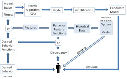
The framework currently uses time-series data from simulations to evaluate models;
however, the framework could be extended to include observations from a real system directly
as shown in figure 3-3 below. Notice how the extension is able to re-use the search algorithm,
model space, and simplification method. The system to model is the real system; a crowd of
people for example. The historical data is observations of the real system. For example, the
historical data of a crowd would be the trajectories of people in that crowd that are extracted
from video of the crowd. Lots of progress has been made towards extracting pedestrian
trajectories from video [11]. The behavior feature functions are functions that are very similar in
purpose and form to the desired behavior functions. A behavior feature function measures some
aspect of a systems behavior. For example, it might measure the density of a crowd. The output
of the behavior feature function is a feature; the specific density of a crowd for example.
Features are then fed into the rest of the framework. When the search algorithm wants to
evaluate the fitness of a model it applies the behavior feature functions to that model and then
have a density similar to the real system. Like the existing modeling process the extended
modeling process has a feedback step where the system to model is compared to the candidate
model. If there is a discrepancy, then behavior feature functions can be added or modified. For
example, the exact mathematical way that density is measured can be tweaked. A modeler might
have to decide between measuring average density, minimum density, maximum density, or
some other variation. The specifics of a behavior feature functions or desired behavior functions
[image:38.612.97.518.268.532.2]are significant.
Figure 3-3 Extending the framework modeling process
3.2 Framework Overview
The simulation modeling framework has three major components: a model space
specification, a search algorithm, and a set of measurement metrics. The model space
specification provides a formal specification for the general model structure from which various
behaviors. Furthermore, it must capture agent behavior in a way that is comprehensible and
human readable. This latter requirement is important because in order for the model space to be
controllable it must be possible for a person to modify a model by hand and know the impact this
will have on behavior. The search algorithm is used to efficiently search the model space for
candidate models that exhibit desired behavior. It must be able to accommodate a variety of
objective functions specifying the search criteria and to discover robust models according to the
criteria. Finally, the framework evaluation metrics are used to evaluate the degree to which the
framework is flexible, robust, comprehensible, controllable, and composable. These
measurement metrics can be used to evaluate an application of the framework to a different
domain or a future extension to the model space specification.
Figure 3-4 Data-driven simulation modeling framework components
This chapter is organized as follows. First the model space specification is described.
Second the model space search method is described. The model space search method section
describes the search process and defines the specific fitness functions used in this chapter and the
next chapter. After that the framework evaluation metrics (flexibility, robustness,
comprehensibility, controllability, and composability) are described in detail. The final section
presents experimental results.
Model
Space
Specification
Model
Space
Search
Framework
Measurement
3.3 Model Space Specification
To support the automated discovery of models a formal model structure is needed. This
section provides a specification of the model space including agents and the world. Each agent
corresponds to a real world mobile agent such as a person, car, or animal. The framework is
designed to represent mobile agents in the abstract, but it can be extended through arbitrary
properties, discussed in detail later, to represent specific kinds of mobile agents such as people.
Each agent takes up a 2D circular space and the world wraps vertically and horizontally. It is also
possible for the environment to bounded by walls and in these scenarios world wrapping is
turned off. Deciding whether a model should wrap or not is consequential because agents'
interactions with walls require learning additional behaviors. Circular impermeable obstacles can
be added to the environment to test the ability of the framework to learn obstacle avoidance
behaviors. In all experiments in this chapter the positions and headings of agents are randomly
set at the start of each simulation and their behavioral rules cause them to organize into collective
patterns. In the lane formation experiments in the next chapter, the agents' positions are
randomized but not the heading.
Formally, a model, m, is composed of a set of entities, E, and a description of the world,
w. In general, each entity has a set of properties, whose values can either be fixed or change
dynamically. The entities are: agents, A, obstacles, O, and zones, Z. Agent entities are able to
dynamically update their angle (also called "heading"), speed, and position properties over time,
i.e., they can move in 2D space. Each agent has a set of behaviors that update the angle and
speed properties. The position property is updated each timestep using the previous position,
heading, and speed as input. Obstacle entities are static entities which act as obstacles in the
represent areas that agents can inhabit. Impermeable zones represent barriers such as walls.
Agent entities can be extended to represent any entities that exhibit certain dynamic behavior or
whose properties can be dynamically updated. For example, it may model an energy source
where the amount of energy dynamically changes over time. Nevertheless, the focus of this
dissertation is on mobile agent movement patterns and thus only the position, angle, and speed
properties are used. The formal model space definition is given below.
m = <E, w>; Model m is composed of a set of entities, E, and the world, w.
w = <width, height>, where the world is a 2-D space that wraps vertically and horizontally
E = {A, O, Z}, where: A is the set of agents O is the set of obstacles Z is the set of zones o ϵ O, where:
o = <x, y, r>, where:
x and y are the coordinates of the obstacle's center r is the radius of the obstacle
z ϵ Z, where:
z = <x, y, w, h>, where:
x and y are the coordinates of the zone's lower left corner
w and h are the width and height of the zone, which is rectangular
3.3.1 Agents
Each agent has their own set of properties and adopts a behavior-based structure to
control how those properties can be changed based on their current value and observations of the
environment and other agents' properties. Although a modeler can design agents to have the
same set of behaviors and properties, as in the models in the results section of this chapter, this is
not forced by the framework. The framework is flexible enough to handle whatever agent
properties the modeler decides to include.
Each agent, a, has its own location, la (also referred to as "position"), heading, ha (also
referred to as "angle"), and speed, sa. The heading is the direction an agent is facing and moving.
heading, and speed of each agent are randomly initialized at the start of a simulation. The
movement vector is intentionally separated into heading and speed to allow each one to be
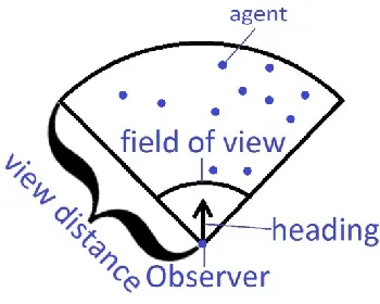
controlled by behavioral rules separately. Each agent has a field of view, fova, defined by an
angle, anglea, and a view distance, viewDistancea, which determines what it sees (figure 3-5
below). Entities can optionally be set as globally visible, which means that agents can see them
regardless of distance. The goal zones in the lane formation experiments in chapter 5 are globally
visible. For modeling flexibility each agent can have its own fov, but in the experiments each
agent has the same fov. This flexibility is important for modeling groups of heterogeneous
agents; for example, a taller person can see further in a crowd than a shorter person. An agent
can perceive all other entities (agents, obstacles, or zones), i.e., know their property values,
within its field of view. Each agent has a set of arbitrary modeler defined properties, Pa. For
example, a model simulating how children follow a teacher on a field trip could have a “type”
property to define agents as either being a student or the teacher. Agents have a set of behavior
groups, BG. Each behavior group, bg, contains one or more behaviors that modify one agent
property. No two behavior groups can modify the same property. All behaviors modifying the
same property belong to the same behavior group. Different agents can have different behavior
groups due to the fact that their properties are different. In the current implementation of the
framework there is a behavior group for the angle and speed properties. The next sub-section
explains the behavior groups in more detail. During a simulation, each agent uses its own
observations and state at timestep t to determine through behavioral rules what its new speed and
heading (and/or any other properties) will be at time t + 1. The position at time t + 1 is projected
from the position at time t using the heading and speed at time t + 1. The formal definition of
a ϵ A
a = <ha, sa, la, fova, Pa, BGa>, where:
ha = heading of agent
sa = speed of agent
la = <xa, ya>; is the location of the agent
fova = <anglea, viewDistancea>; is the field of view of the agent
Pa = set of arbitrary modeler defined properties
[image:43.612.237.412.209.349.2]BGa = set of behavior groups, where bg ϵ BGa
Figure 3-5 An agent's field of view determines what entities (agents, obstacles, and zones) it can see
3.3.2 Behavior Groups
An agent can have multiple behavior groups where each behavior group, bg, contains
behaviors that modify one agent property. Behavior groups give the model space specification a
general way of modifying agent properties. No two behavior groups can modify the same agent
property, and all behaviors modifying the same property belong to the same behavior group.
Behavior groups can modify an agent's heading, speed, and arbitrary modeler defined properties.
A behavior group is composed of the name of the property a behavior group modifies, pbg, a set
of behaviors, Bbg, and a set of weights, Wbg, for those behaviors. For the experiments in chapter
4, one behavior group is used for angle and another for speed. If other agent properties were
modified, then each of these would also belong to an associated behavior group. If an agent's
behavior group is empty for a particular property than the default property value is used. In the
max speed, which was chosen instead of the current speed in order to bias agents towards
movement. The default speed behavior will become significant in the results section when it
plays a critical role in establishing personal space between agents.
bg = <pbg, Bbg, Wbg>; is a specific behavior group, where:
pbg is the property the behavior group modifies, where:
no two behavior groups can modify the same property pbg refers to ϵ {ha, sa} ∪ Pa
Bbg is the set of behaviors, where b ϵ Bbg
Wbg is the set of weights, where:
w ϵ Wbg
w ≥ 0 |Wbg| = |Bbg|
∑(Wbg) = 1
A behavior, b, in a behavior group, bg, corresponds to one influence on one property of
an agent. In the real world it might correspond to a behavior like; avoid hitting another
pedestrian. The multiple behaviors belonging to the same behavior group will have a compound
influence on the property the behaviors influence. In the current framework, this compound
influence is based on a weighted average calculation. As described above, each behavior has an
associated weight. A behavior group calculates the weighted average of these competing
influences from all behaviors belonging to the behavior group to decide the compound influence.
A behavior can be activated or not (more on this later), if no behaviors in a behavior group are
activated, then the corresponding default behavior is chosen.
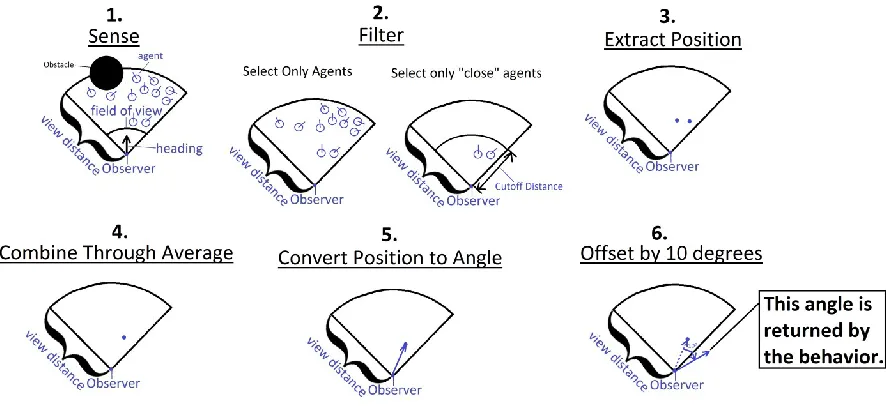
3.3.3 Behaviors
A behavior is a general way of describing what entities in the environment are used to
make a decision (filtering), what property of the relevant entities will be used (extract), and how
to act given the property values of the relevant entities (combine and offset). A behavior
contains: the category of entities it considers, Cb, the set of types within that category it
combination function, Combineb, and an offset to add to the result of the combination, Offsetb.
An example of applying a behavior is illustrated in figure 4 below. After observed entities have
been filtered by category and type the general filters, Fb, decide what entities a behavior will use.
Notice in the equations below that filters can be "chained." For example, select all agents within
a distance of 10 with a speed slower than 2. Chained filters are flexible while still remaining
comprehensible. The property extraction step decides what property of the used entities will be
used to make a decision; any property can be used. The combination step combines the extracted
properties, so that one decision can be made from multiple observations. The combination
methods are shown in table 3-1; note that currently angle, speed, and position are the only
extractable properties currently used; however, the framework could be extended to include
arbitrary properties. The offset step offsets the combined property value to allow for more
nuanced behaviors. Offsets can be negative or positive. Positive and negative angle offsets refer
to different turning directions. Frequently the sign of the angle offset is not significant because
the modeler does not care whether agents prefer turning left or right. The sign of the speed offset
is always significant because it either slows down or speeds up an agent. The formal definition of
a behavior is given below:
b = <Cb, Tb, Fb, Extractb, Combineb, Offsetb>, is a specific behavior where:
Cb is the category of entity the behavior accepts; it is either: agents,
obstacles, or zones
Tb is a set of types of entity, within a category
Fb is the composition of filter functions, where:
Fb(Esense) = (fp,r,1∘ fp,r,2∘ ... ∘ fp,r,n)(Esense), where:
Esense⊆ E, where Esense is the set of entities that are sensed by an
agent
fp,r,i is the i'th filter, where:
p is the value of the filter property being used for filtering
r is the range that p must be within for the entity to pass the
filter
Extractb is the property extraction function
offsetb is the offset; it can be positive or negative
Figure 3-6 Example of behavior that turns the observing agent 10 degrees away from nearby agents
Table 3.1 Property combination functions for: position, angle, and speed Absolute
combination
Relative (to observer) combination
angle average, random Closest (most similar to observer's heading),
farthest
speed average,
random, fastest, slowest,
closest (most similar to observer's speed), farthest (most dissimilar speed)
position average, random farthest, closest
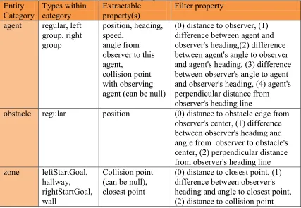
In table 3-2, below, for each entity category the possible types, extractable properties, and
filter properties are listed. The table lists the values used in the experiments, but it should
stressed that this is a general framework, so it is easy to add additional types, arbitrary properties,
and additional filters if desired. For example, the model space could be extended to include types
for "youngChild" and "parent" to build models where a young child is following their parent
[image:46.612.120.563.116.319.2]