PILE DESIGN USING MULTIPLE LINEAR REGRESSION MODEL
Nabeel S. Juwaied and Faiq Mohammed Sarhan Al-Zwainy
Department of Civil Engineering, College of Engineering, Al-Nahrain University, Baghdad, Iraq
E-Mail: [email protected]
ABSTRACT
There is a marked increase in the use of statistic and its methods in representing the complex relationship between factors in geotechnical engineering. In this paper “Multiple Linear Regression” model, has been developed to produce a pile design equation. Using data from in situ full scale drilled shaft and driven pile test. The objective of this study is to use simple data from widely use tests, at an early stage of pile design, to develop (MLR) model. SPT-N values and the geometrical properties were the simple data. The MLR model developed for pre-stressed reinforced concrete pipe pile, cast in place reinforced concrete pile and precast square driven reinforced concrete pile. A database of 63 historical cases collected from five projects in Iraq/Baghdad to be the reference to the current method of pile design equation. The resulting equation was used to find the prediction design load of the pile and compare it with the actual. The results showed relatively high correlation coefficient r, 96% between the actual and predicted values. AS an application to confirm equation accuracy, 7 cases not use in the model development were taken, the results showed high correlation coefficient r, 97% and coefficient of determination r2, 94% between the actual and predicted values.
Keywords: multiple linear regression, piles, axial load, design.
1. INTRODUCTION
Generally, a pile design is prediction method to the actual behavior of pile. There are many methods and approaches for the prediction of the axialbearing capacity of driven and bored piles. However, all these methods based on some streamlining assumptions or incorrectly ruminate the effect of certain main factors as soil-pile structure interaction, distribution of soil resistance along a pile, and soil stratigraphy.
Most geotechnical problems are complex. Due to the behavi or of piles governing by large number of uncertain parameters, in- situ full scale pile load test is almost precise way to check the actual performance of pile. An important indication of pile load-carrying capacity obtained from a load test is the pile load-settlement curve. But, in fact to determination clearly pile bearing capacity, or failure load based on a load-settlement curve, there is no single standard. To evaluating the "failure" load of a pile, several methods have been proposed, and they producea very wide range of results (Horvitz et al., 1981). So, they don’t provide directly useable values in the design of foundation. Therefore, pile design seems to be somewhat of a guessing game rather than be a subjective exercise (Shariatmadari et al., 2008).
2. AXIAL PILE CAPACITY
The prediction of pile capacity always has been a problematic and a big challenge to geotechnical engineers. To deal with the uncertainty in the prediction, many approaches and methods were developed. Generally, there are three main groups of categories to estimate axial pile capacity (Nawari et al, 1999):
a) Full-scale load tests.
b) Static methods, analysis based on soil properties from laboratory or in-situtests.
c) Dynamic methods, analysis based on pile driving dynamics.
Each of these methods has characteristics of strength and weakness but neither one is entirely acceptable. Accordingly, designers usually tend to use more than one method and the final design will be a synthesis of the results.
Most dependable design is based on the results from approach (a). Though, static load tests are costly and time consuming. The static formulas (e.g. Meyerhof-Method, b -method, a -method, g -method … etc.) in approach (b) produce pile with low efficiency and poorly relate with the static load test.
In approach (c), there are largely empirical in the definition of the soil-pile interface models (Nawari et al,
1999).
3. PILE DESIGN BASED ON IN-SITU TEST RESULTS
The application of in-situ tests to pile design can be done through indirect or direct methods. Indirect methods use the in-situ test results to evaluation of the soil characteristic parameters, such as the internal friction angle Ø and the undrained shear strength Su. This requires consideration of complicated boundary-value problems (Campanella et al., 1989). Instead, direct methods, use of the results from in-situ test measurements for the analysis and the design of foundations without the evaluation of any soil characteristic parameter. However, the application of direct methods to the analysis and the design of foundations is, usually based on empirical or semi empirical relationships. Indirect pile design methods (e.g. Vesic (1977), Coyle and Castello (1981), P method (Burland 1973) for cohesionless soil, …etc.) mostly define the correlation factor between the stress state based on the soil-strength parameters and base or shaft resistance.
in-situ testing techniques recently has increased for geotechnical design. That was as a result of quick development of in-situ testing apparatuses, a better understanding of the behavior of soils, and successive realization of some restrictions and insufficiencies of conventional laboratory testing (Lunne et al., 1997).
The cone penetration test (CPT) and standard penetration test (SPT) were commonly usedbased on the approach on in situ testing. The two tests are most in situ test which commonly using in direct methods for pile design. In CPT test, a cylindrical penetrometer with a conical tip is pushed into the ground. There is good similarity between the pile loading and cone penetration testing mechanisms. So, the CPT is an outstanding test for pile design purposes.
Furthermore, its ability of simultaneous measurement of shear wave velocities makes it potential to estimate elastic properties of subsurface soils, and that could make the design more accurate for determine in-situ soil properties.
SPT has a number of limitations (Seed et al. 1985, Skempton 1986). The main limitation is the measured SPT-N values are not well related to the pile loading process. However, utilizing SPT test results is very important, because it is more extensively used all over the world.
4. AXIAL PILE BEARING CAPACITY FROM (SPT) As a result of the complexity and the uncertainty related to geotechnical field, no adequate solution or general procedure for the estimation of the pile capacity from simple soil tests is available.
One of the earliest applications of the SPT test is the determination of pile capacity. That includes two main approaches, direct and indirect methods (Nayak, 1985). Direct methods apply some modification factors with N values. However, considerable uncertainty exists about filtering and averaging the data relating to pile resistance, pile base failure zone, use of total stress approaches, and capacity of piles with limited base penetration in dense strata. Indirect SPT methods employ a friction angle and undrained shear strength values estimated from measured data based on different theories. In indirect methods, only soil parameters are obtained from SPT results and the methodology of the pile bearing capacity estimation is the same as for the static methods, and therefore involves the same sources of shortcomings (Eslami & Fellenius, 2004).
5. INTERPRETATION AXIAL PILE CAPACITY FROM LOAD-SETTLEMENT CURVES
As mention previously, to evaluating the capacity of a pile from in situ load test, several methods have been proposed, and they produce a very wide range of results. Most commonly used methods that proposed for interpretation of pile load-settlement curves (Brinch Hansen, 1963: 90% and 80%), (Butler and Hoy, 1977 or tangent method), (Chin 1970), (Davisson 1972), (De Beer, 1967), and (Decourt Extrapolation). This study will not discuss the details of these methods.
The results of application these methods to interpreting the capacity of the pile (PA-14-2) which it on of data case records that will use to development the models of this study, are presented in Table-1.
We can see from Table-1, the Pile (PA-14-2) has widely different interpretation values of bearing capacity, ranging from 707.2 KN to 7125.7 KN.
Table-1. Estimation the ultimate pile (PA-14-2) capacity.
Method Ultimate bearing
capacity, KN Tangent Method Over 2400
Chin Method 2610
Davisson Method Over 2400
De Beer Method Over 2400 Decourt Extrapolation
Method 7125.7
Hansen Method 707.2
6. DATA BASE AND CASE RECORDS
An extensive search of projects in Iraq at last two decades was conducted to collect axially loaded piles and SPT, resulted in a large number of cases. A data base was established from case histories including SPT, soil characteristics and result of full-scale pile loading test.
Many of the cases involved limitations, for example SPT results with not specified energy ratio of N values which cannot produce accurate measurements, manually smoothed and filtered SPT data, incomplete results of pile loading tests, not proper location or depth of borehole, etc. Thus, selection criteria are necessary to create a database of case histories pile tests and SPT preformed close to the pile locations.
6.1 Selection criteria
The following selection criteria were applied to the case histories:
a) SPT test must be performed close to the piles locations.
b) SPT data must be available along the pile and at least four pile diameters beneath the pile toe.
c) SPT data must be measured in uniform distance, from spacing not more than 2 m and at least one measurement for each different layer and record the average of every intervals depth.
d) Sites must include sediments of clay, silt and sand soil layers.
e) Pile loading tests must be reached the design loads, which is the structure’s working loads multiple by suitable factor of safety.
f) Pile shafts must have constant cross sectional area.
g)
Piles must be subjected to the axial compressionloads.
information was missing. The work resulted in total of (63) pile case histories from 5 sites.
The compiled database includes five sites, obtained from projects in /or near Baghdad. Table-2 summarizes the case histories location characteristics including site, and number of cases.
The brief information of the projects selected in, is presented below:
a. Bismayah new city - National housing program BNCP is the first and the biggest city development project throughout the history of Iraq. Bismayah city is located 10km south east of Baghdad on the Iraqi-Kuwaiti Highway, spread on a total area of 1,830-hectare area and is planned to accommodate around 600,000 occupants in a total of 100,000 residential units. Also the infra-network such as electricity, water supply, and streets will be constructed. As well as the infra-network.
b. Amriah residential compound- National housing program
The project is one of the Iraqi housing program in Baghdad. Consists of many groups of six story residential buildings in a total of 952 residential units. As well as the infra-network.
c. Paralympic headquarter
The project of construction the Iraqi Paralympic committee head quarter in Baghdad, six stories buildings with an area of 3304 m2.
d. International hotel
The project of construction a five stars’ hotel and mall in Baghdad. 16 stories buildings spread on a total area of 20000 m2, at the bank of Tigris river.
e. Imam –Ali hospital
The project of construction more than 250 beds government hospital. Six stories buildings, in “ Al-Rusafa”/Baghdad.
Table-2. Summary of case histones site locations.
No. Project Number of cases
1 Bismayah New City 10
2 Amriah Residential
compound 7
3 Paralympic Headquarter 3
4 International Hotel 13
5 Imam Ali Hospital 27
6.2 Pile characteristics
The 63 concrete plies collected for the database, range in dimension from 285mm in square piles, through diameter 1000 mm and range in embedment length from 7.25m through 24.5m.
The shapes of cases are pipe, square, round. The majority shape of pile is round. More than seventy percent of pile case histories are bored piles and the remaining are driven piles.
6.3 Pile loading tests
Axial compression static load test was performed on all of the piles in the database. The piles were loaded in slow increment load procedures. The piles were tested by applying the axial load at the corresponding elevation of the piles cap heads. Steel platform was used to transfer the applied load from the jack to tested pile which loaded to a (2-3) of the proposed working load.
The apparatus of applying compressive loads for all pile testing and the procedure of increment load and settlement reading were carried out according to (ASTM D1143-81) (Reapproved 1994).
Figure-1. Typical pile load test results within database.
6.4 Soil information
The sources for soil interpretation were the boring; sampling; laboratory testing results, and in-situ testing particularly the SPT. The case histories involve sites with soils generally varying from soft clay to fine gravel with silt or sand.
6.5 Standard penetration tests
The measured SPT data represent total stress. For a study based on effective stress, it is necessary to measure the pore pressure. The detailed soil profiles must be based on SPT measurements at short spacing as possible, and at least one measurement for each different layer.
Figure-2. Typical SPT diagram within databank.
7. MULTIVARIABLE LINEAR REGRESSION MODEL
(MLR) has been used to developed statistical model for produce design equation for compressive axially loaded pile. The suggested (MLR) model is supposed to use simple soil field test, standard penetration test (SPT) to determine pile design capacity. This makes the model attractive to designers (both structural and geotechnical) plus researchers.
Regression analysis, is a statistical process for estimating the relationships between variables, i.e. estimate the association between one or more explanatory
variables and a single outcome variable.
The objectives of a regression analysis are to predict or explain differences in values of the outcome variable with information about values of the explanatory variables (Hoffmann, 2010). The mainly interested of regression issues in this study are:
a) The form of the relationship or the equation that represents the relationship among the outcome and explanatory variables.
b) The direction and strength of the relationships. c) Predicting a value of the outcome variable for a given
set of values of the explanatory variables.
In the simple linear regression model, there are only one explanatory and one outcome variable. Figure-3 showed this relationship and can represented in equation as:
y= β0+ β1xi (1)
y= β + (tan Ø)xi (2)
where the β1represented the slope and the β0represented the point at which the line crossed the y axis, or the intercept.
Figure-3. Linear regression modelling.
Almost any two variables used in the behavioral sciences will fail to line up in a scatter plot. actual relationship between the variables misrepresents by above equation, so as it far off exactness. The straight line is, at best, an approximation of the actual linear relationship between x and y. However, linear regression equation must revise to consider the uncertainty of the straight line. Statisticians have therefore introduced what is known as the error term into the model (Hoffmann, 2010):
y= β0+ β1xi+εi (3)
The letter εrepresents the uncertainty in predicting the outcome variable with the explanatory variable.
In the Multiple Linear Regression Analysis, is linear regression models that include more than one explanatory variable. Usually there are many potential explanatory variables used to predict an outcome variable. Equation (4) represented the general form ofMultiple Linear Regression equation:
y= β0+ β1x1+ β2x2+.... +βpxip+ εi (4)
where:
i= 1,2, 3, …, n; xiis the response that corresponds to the levels of the explanatory variables x1, x2, …, xp at the ith observation.
β0, β1, …, βp are the coefficients in the linear relationship.
ε1,ε2, …,εi are errors that create scatter around the linear relationship at each of the i = 1 to n observations.
The regression model assumes that these errors are mutually independent, normally distributed, and with a zero mean and variance σ2 (Al-Zwainy et al., 2013)
8. SPT-VALUE AVERAGING
proper unit shaft and base resistances it is very important to consider the variations of soil resistance properties by presenting an average value for N. As unit shaft and base resistances are related to the average value of N, this value should be a relevant representative. Commonly two methods of averaging, arithmetical and geometrical, are used to find the mean value of a series of numbers.
The arithmetical average is calculated as follows:
𝑁𝑎= 𝑁 +𝑁 +⋯+𝑁𝑛 𝑛 (5)
Where Nais the arithmetical average of N1to Nn.
The geometrical average (geo mean) is calculated as follows:
𝑁𝑔= 𝑁 + 𝑁 + ⋯ + 𝑁𝑛 ⁄𝑛 (6)
Where Ngis the geometrical average of N1 to Nn.
For example, 25 and 16.35 are the arithmetic and geometric averages, respectively for the data as follows, 4, 6, 11, 14, 15, 16, 15, 19, 60 and 90. This example proves that the value of the geometric average is closer to the main average value of these numbers, since the arithmetic value is highly affected by values of 60 and 90. So, using the geometrical average method to obtain the logical representative of N values seems to be more accurate and relevant (Eslami & Fellenius, 1997).
The SPT values used for the geometric average should be as possible at a constant spacing.
To obtain the unit base resistance of piles from standard penetration test results, the failure zone and failure mechanism should be specified around the base of the pile. The purpose is the simulation of the punctuate failure at the bottom of the pile. (Eslami & Fellenius, 1997) represented simulation of the local failure, which is a spiral logarithmic surface starting at the base of the pile, and ending at one point on its body.
The height and depth of this spiral logarithmic surface can vary between four to nine times the pile diameter (4-9 D) at the upper part of the pile, and between one and 1.5 times the pile diameter (1-1.5 D) below the base, depending on the soil friction angle. In case the confining soil is heterogeneous, this failure pattern cannot
be generalized for the failure that occurs around the pile base (Figure-4). (Shariatmadari et al., 2008) developed model regarding the geometric mean of N-values around the pile, failure zone extending 8D above, and 4D below the pile base.
In this study, used a geometrical average value for N between four times the pile diameter (4D) below the base, and the geometrical average of the N values along the pile length at the upper part of the pile.
Figure-4. Schematic view of spiral logarithmic failure surface around the base. (Eslami & Fellenius ,1997).
9. MODEL FACTORS IDENTIFICATION
The multivariable linear regression (MLR) developed in this chapter used as independent variables geometrical averaging (SPT-N) values, embedment length of pile in soil, pile cross section area, pile tip area, pile perimeter, main reinforcement area and settlement of pile at pile design capacity.
Pile design capacity was the dependent variable of model.
The statistic of the data used are given in Table-3.
Table-3. Ranges of the data used in MLR model.
Model variables Minimum Maximum Range Mean Standard
deviation
Penetration depth, L (m) 7.25 24.50 17.250000 17.641071 3.3135
SPT-N Value 11.94 32.61 20.666613 23.208809 8.0701 Tip area, Atip(m
2
) 0.081200 0.79 0.704200 0.316374 0.1628
Cross-sectional area, Asec(m2) 0.081200 0.79 0.704200 0.306300 0.1741 Perimeter, Pr(m) 1.1400 3.14 2.002000 1.616335 0.6320
Area of steel, As (m2) 0.000512 0.01 0.007344 0.002989 0.0016 Settlement, St (m) 0.0020 0.08 0.072960 0.009639 0.0111
9.1 Development mathematical models using MLR technique
The variables were used to develop the Multiple Linear Regression (MLR) model. The Statistical Product and Solutions Services (SPSS) software versions 20 are used as a tool to develop the regression model. From results of the analysis of variance (ANOVA). The F-test of model is highly significant, thus we can assume that there is a linear relationship between the variables in our model, i.e. the model can predict the pile capacity by the input variables. So, we can reject the null hypothesis that “The model has no predictive value.”
9.2 Regression model equation
Regression equation is in form of equation (4). MLR model coefficients from (SPSS), used to predicting pile design capacity.
So, the MLR equation after simplified will be as:
Qdes = 180L-5N + 993 Atip–11047Asec+3012Pr+ 366833 As
+ 3348 St- 4042 (7)
Where:
Qdes = Pile design capacity,KN
L = total embedment length of the foundation pile that is in contact with soil, m.
N = geometric average of SPT-N values along the full embedment length of pile in soil (in our calculations N are equal to ((N1)60) by standard penetration test).
Atip = pile tip area, m 2
Asec = pile material cross sectional area, m2
Pr = pile perimeter, m.
As = area of main longitudinal reinforcement, m 2
.
St = settlement of pile, m.
Model performance and validation
The final MLR equation 7 was used to predict the pile design capacity using the two subset of data. Table-5 presented the actual and predicted values of pile design capacity by using the validation dataset.
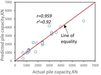
The performance of the MLR model for tow dataset is given in Table-6. It can be seen from this table that the MLR model performed well. Where about 92% of change in pile design capacity values can explain by the model input variables. And there is relatively high correlation coefficient r, 96% between the actual and predicted values.
For the validation dataset, the equation result showing very high correlation coefficient r, 97% and coefficient of determination r2, 94% between the actual and predicted values. Most popular error measure is the
RMSE and has The advantage that large errors receive much greater attention than small errors ((Hecht- Nielsen 1990) However, according to Cherkassky et al. (2006), RMSE cannot always guarantee thatthe model performance is optimal, thus, MAE was also used to eliminates the weight given to large errors, and isnecessary
Table-4. Actual and predicted values of MLR model for pile design capacity.
Case No.
Actual Pile design capacity (Kn)
Predicted Pile design capacity
(Kn)
1 1600 2197.9
2 1600 1954.5
3 3200 3231
4 3200 3202.7
5 700 464.4
6 1200 1291.8
7 1200 1174.2
Table-5. Analytical performance of MLR model for pile design capacity.
Performance measure
Model dataset
Validation dataset
r 0.959 0.96
r2 0.92 0.93
RMSE 304 280
MAE 165 191
In Figures 5, 6 comparison of the predicted pile load capacity using MLR model for tow dataset and their deviation from actual has been made.
0 1000 2000 3000 4000 5000 6000 7000
0 1000 2000 3000 4000 5000 6000 7000
Predi
cted
p
il
e
ca
p
aci
ty
,KN
Actual pile capacity,KN Fig. 5. Comparison of predicted and actual design piles capacity for model dataset
Line of equality r=0.959
[image:6.595.324.531.467.621.2]10. CONCLUSIONS
Simulating the complex behavior of soil as an attempt to infer the response of the soil-structure system involves many degrees of uncertainty.
Multiple linear regression model was introduced for the design of piles subjected to axial compression load. The design equation represents the relationships between many variable of soil-structure factors to predict the soil and pile behavior based on actual data. The actual behavior of the piles is determined from full- scale axial static load test in five projects in Iraq at last twenty years.
Apply of the resulting pile design equation for predicted pile design capacity demonstrated that the MLR model has the ability to predict pile design capacity with an acceptable degree of accuracy. Furthermore, the design equation can be used as an accurate and quick tool for pile design. Because it need simple data, mainly SPT-N values and the geometrical properties.
REFERENCES
Aoki N. & De’Alencar D. 1975. An approximate method to estimate the bearing capacity of piles. Proceeding of the Fifth Pan-American Conference on Soil Mechanics and Foundation Engineering, Buenos Aires, Argentina. pp. 367-376.
Faiq Mohammed Sarhan Al-Zwainy, Mohammed Hashim Abdulmajeed, Hadi Salih Mijwel Aljumaily. 2013. Using Multivariable Linear Regression Technique for Modeling Productivity Construction in Iraq. Open Journal of Civil Engineering. 3: 127-135.
Bazaraa A. R. & Kurkur M. M. 1986. N-values used to predict settlements of piles in Egypt. Proceedings of In Situ ’86, New York, pp. 462-474. Blackie Academic & Professional (1997).
Briaud J. L. & Tucker L. M. 1988. Measured and predicted axial capacity of 98 piles. ASCE, Journal of Geotechnical Engineering. 114(9): 984-1001.
Cherkassky V., Krasnopolsky V., Solomatine D.P. and Valdes J. 2006. Computational intelligence in earth sciences and environmental applications: issues and challenges. Neural Networks. 19(2): 113-121.
Campanella, L G., Robertson, P. K, Davies, M. P. and SY A. 1989. Use of in-situ tests in pile design. Proceedings of 12th International Cuiifcience on Soil Mechanics and Foundation Engineering, ICSMFE, Rio de Janeiro. 1: 199-203.
Eslami A. & Fellenius B. H. 1997. Pile capacity by direct CPT and CPTu methods applied to 102 case histories. Canadian Geotechnical Journal. 34: 886-904.
Eslami A. & Fellenius B. H. 2004. CPT and CPTu data for soil profile interpretation: review of methods and a proposed new approach. Iranian Journal of Science and Technology, Transaction B. 28(B1): 69-86
Gregory B. Baecher and John T. Christian. 2003. Reliability and Statistics in Geotechnical Engineering. 2003. John Wiley & Sons Ltd, The Atrium, Southern Gate, Chichester, West Sussex PO19 8SQ, England.
Hecht-Nielsen R. 1990. Neurocomputing. Reading, MA: Addison- Wesley Publishing Company.
Horvitz G.E., Stettler D.R. and Crowser J.C. 1981. Comparison of Predicted and Observed Pile Capacity. Proceedings of a Session Sponsored by the Geotechnical Engineering Division at the ASCE National Convention. pp. 413 - 433.
John P. Hoffmann. 2010. Linear Regression Analysis: Applications and Assumptions Second Edition.
Meyerhof G. G. 1976. Bearing capacity of settlement of pile foundations. The Eleventh Terzaghi Lecture, ASCE Journal of Geotechnical Engineering. 102(GT3): 195-228.
N. Shariatmadari1, A. Eslami and M. Karimpour-Fard1. 2008. Bearing Capacity of Driven Piles in Sands from Spt–Applied To 60 Case Histories. Iranian Journal of Science & Technology, Transaction B, Engineering. 32(B2): 125-140.
Nawari N.O., Liang R., Nusairat J. 1999. Artificial intelligence techniques for thedesign and analysis of deep foundations. Electronic Journal of GeotechnicalEngineeringhttp://geotech.civeng.okstate.edu/ ejge/ppr9909/index.html.
Nayak N.V. 1985. Foundation design manual. Dhanpat Rai & Sons pub.
0 1000 2000 3000 4000
0 1000 2000 3000 4000
Predi
cted
p
il
e
ca
p
aci
ty
,KN
Actual pile capacity,KN
Fig.6 Comparison of predicted and
actual design piles capacity for
validation dataset
Line of equality r=0.96
Rausche F., Goble G. & Likins G. 1985. Dynamic determination of pile capacity. ASCE, Journal of Geotechnical Engineering. 111(3): 367-383.
Schnaid F. 2009. In Situ Testing in Geomechanics, 1st Edition, Taylor and Francis, London, New York, USA.
Shioi Y. & Fukui J. 1982. Application of N-value to design of foundation in Japan. Proceeding of the Second European Symposium on Penetration Testing, Amsterdam. 1: 159-164.
Skempton A. W. 1986. Standard Penetration Test Procedures and the Effects in Sands of Overburden Pressure, Relative Density, Particle Size, Ageing and Over consolidation. Geotechnique. 36(3): 25-447.
Seed B., Tokimatsu K., Harder M and Chung. 1985. Influence of SPT Procedures in Soil Liquefaction Resistance Evaluations. Journal of Geotechnical Engineering, ASCE. 111(12): 1425-1445.