Distributed Load Control in Multiphase Radial Networks

(1)

Distributed Load Control in Multiphase Radial Networks

Thesis by

Lingwen Gan

In Partial Fulfillment of the Requirements for the Degree of

Doctor of Philosophy

California Institute of Technology Pasadena, California

2015

(2)

c

2015

(3)

The thesis is dedicated to my girlfriend Tianlu, whose love made this thesis possible,

and my parents,

(4)

Acknowledgements

I would like to express my deepest gratitude to my advisor, Professor Steven Low, who guided me through my years pursuing a Ph.D. He is shockingly nice and always places his students first: he allowed me to graduate ahead of time when I fell into financial crisis, he never pushed us to work for the funding, he allowed us to work from home, and he took care of a lot of dirty work himself. He is enthusiastic about research and always works on hard-core problems: he digs into the details of our work and thinks with us along the way, he consistently brings us onto the right track, and encourages us to take risks and aim big in our careers.

Next, I am grateful to my collaborators, Ufuk Topcu, Adam Wierman, Na Li, and Niangjun Chen. It is a great pleasure to work with and take the advice of these great minds. Professor Ufuk Topcu is the first person who taught me how to write a technical paper. Professor Adam Wierman taught me how to make a technical paper easy to read, and how to make a decent presentation (though I never even got close to his level).

I have greatly enjoyed studying in the department of Electrical Engineering at California Institute of Technology. We are provided an amazing working and living environment. The large and bright three-people offices are paradise for theoretical research, and all sorts of free lunches and snacks have provided us with great relaxation. I would also like to thank the helpful administrative staff, Christine Ortega, Lisa Knox, and Sydney Garstang, and many others.

I would like to thank my parents for their spiritual support during the years. They have gone through extremely difficult times: an illness that pushed us to the edge of despair, bad relationship with relatives, and grudge from the elders. Even during the most difficult times, they encouraged me to pursue my dream of being a scholar without worrying about their well-being. I know it is absolutely my duty to take care of their needs.

(5)

Abstract

The current power grid is on the cusp of modernization due to the emergence of distributed gener-ation and controllable loads, as well as renewable energy. On one hand, distributed and renewable generation is volatile and difficult to dispatch. On the other hand, controllable loads provide signifi-cant potential for compensating for the uncertainties. In a future grid where there are thousands or millions of controllable loads and a large portion of the generation comes from volatile sources like wind and solar, distributed control that shifts or reduces the power consumption of electric loads in a reliable and economic way would be highly valuable.

Load control needs to be conducted with network awareness. Otherwise, voltage violations and overloading of circuit devices are likely. To model these effects, network power flows and voltages have to be considered explicitly. However, the physical laws that determine power flows and voltages are nonlinear. Furthermore, while distributed generation and controllable loads are mostly located in distribution networks that are multiphase and radial, most of the power flow studies focus on single-phase networks.

This thesis focuses on distributed load control in multiphase radial distribution networks. In particular, we first study distributed load control without considering network constraints, and then consider network-aware distributed load control.

Distributed implementation of load control is the main challenge if network constraints can be ignored. In this case, we first ignore the uncertainties in renewable generation and load arrivals, and propose a distributed load control algorithm, Algorithm 1, that optimally schedules the deferrable loads to shape the net electricity demand. Deferrable loads refer to loads whose total energy con-sumption is fixed, but energy usage can be shifted over time in response to network conditions. Algorithm 1 is a distributed gradient decent algorithm, and empirically converges to optimal de-ferrable load schedules within 15 iterations.

(6)

time step, and its total energy consumption equals the expectation of future deferrable load total energy request.

Network constraints, e.g., transformer loading constraints and voltage regulation constraints, bring significant challenge to the load control problem since power flows and voltages are governed by nonlinear physical laws. Remarkably, distribution networks are usually multiphase and radial. Two approaches are explored to overcome this challenge: one based on convex relaxation and the other that seeks a locally optimal load schedule.

To explore the convex relaxation approach, a novel but equivalent power flow model, the branch flow model, is developed, and a semidefinite programming relaxation, called BFM-SDP, is obtained using the branch flow model. BFM-SDP is mathematically equivalent to a standard convex re-laxation proposed in the literature, but numerically is much more stable. Empirical studies show that BFM-SDP is numerically exact for the IEEE 13-, 34-, 37-, 123-bus networks and a real-world 2065-bus network, while the standard convex relaxation is numerically exact for only two of these networks.

Theoretical guarantees on the exactness of convex relaxations are provided for two types of net-works: single-phase radial alternative-current (AC) networks, and single-phase mesh direct-current (DC) networks. In particular, for single-phase radial AC networks, we prove that a second-order cone program (SOCP) relaxation is exact if voltage upper bounds are not binding; we also modify the optimal load control problem so that its SOCP relaxation is always exact. For single-phase mesh DC networks, we prove that an SOCP relaxation is exact if 1) voltage upper bounds are not binding, or 2) voltage upper bounds are uniform and power injection lower bounds are strictly negative; we also modify the optimal load control problem so that its SOCP relaxation is always exact.

(7)

List of Figures

2.1 Base load profile is the average residential load in the service area of Southern California Edison from 20:00 on February 13, 2011 to 9:00 on February 14, 2011 [2]. Optimal total load profiles correspond to the solutions of the ODLC problem (2.5). With different EV specifications, optimal charging profiles can be valley-filling (left figure) or non-valley-filling (right figure). Hypothetical non-optimal total load profiles are shown in purple with dash-dot lines. . . 12 2.2 An example of equivalent charging profiles. In both top and bottom figures, the red

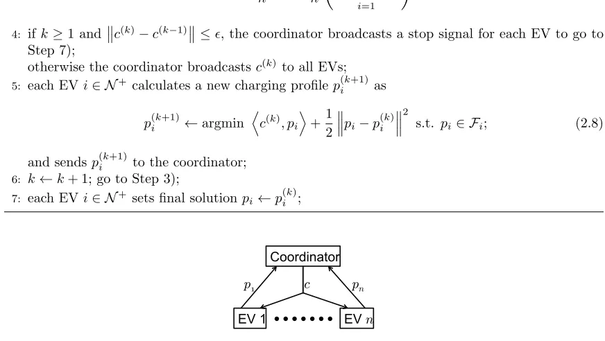
region corresponds to the charging profile of one EV, and the blue region corresponds to the charging profile of another EV. The total load profiles in both figures equal, therefore the charging profiles in both figures are equivalent. . . 12 2.3 Schematic view of the information flow between the coordinator and the EVs. Given the

control signalc, EVs update their charging profilespi independently. The coordinator

guides their updates by altering the control signalc. . . 14 2.4 All EVs plug in at 20:00 with deadline at 9:00 on the next day, and need to charge

10kWh electricity. Multiple purple dash-dot curves correspond to the total load profiles in different iterations of Algorithm MCH. . . 18 2.5 All EVs plug in at 20:00 with deadline at 9:00 on the next day, but need to charge

different amounts of electricity that is uniformly distributed between 0 and 20kWh. . 18 2.6 All EVs need to charge 10kWh electricity, but plug in at different times (uniformly

distributed between 20:00 and 23:00) with different deadlines (uniformly distributed between 6:00 to 9:00 on the next day). . . 19

3.1 Diagram of the notation and structure of the model for base load, i.e., non-deferrable load minus renewable generation. . . 22 3.2 Illustration of the traces used in the experiments. (a) shows the average residential

(12)

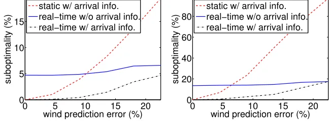
3.3 Illustration of the impact of wind prediction error on suboptimality of load variance. . 37

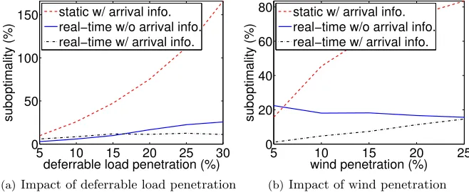
3.4 Suboptimality of load variance as a function of (a) deferrable load penetration and (b) wind penetration. In (a) the wind penetration is 20% and in (b) the deferrable load penetration is 20%. In both, the wind prediction error looking 24 hours ahead is 18%. 38 4.1 Summary of notations . . . 50

4.2 The left figure illustrates the set_Si of an inverter, and the right figure illustrates the setSi of a shunt capacitor. Note that the setSi is usually not a box, and thatSi can be nonconvex or even disconnected. . . 51

5.1 Some of the notations. . . 71

5.1 The busi_∧jdenotes the joint of busiand busj. The resistanceRi denotes the total resistance of the red solid line segment. . . 75

5.2 Buses down(i) downstream of busi lies in the shaded region. . . 86

5.3 Flow chart illustrating the distributed implementation of Algorithm 7. . . 89

5.1 Topologies of the SCE 47-bus and 56-bus networks [35, 37]. . . 102

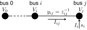
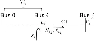
6.1 Some of the notations. . . 107

6.1 Illustration of ˆSij and ˆvi. The shaded region is downstream of busi, and contains the buses{h:i ∈ Ph}. Quantity ˆSij(s) is defined to be the sum of bus injections in the shaded region. The dashed lines constitute the pathPi from busito bus 0. Quantity ˆ vi(s) is defined asv0plus the terms 2Re(¯zjkSˆjk(s)) over the dashed path. . . 110

6.2 We assume that_Si lies in the left bottom corner of (pi, qi), but do not assume thatSi is convex or connected. . . 111

6.3 The shaded region denotes the collection_Lof leaf buses, and the path_Pl of a leaf bus l_{∈ L}is illustrated by a dashed line. . . 112

6.4 A 3-bus linear network. . . 112

6.5 A linear network for the interpretation of Condition C1. . . 114

6.1 Comparison of the computation times for SOCP and SDP. . . 119

6.2 Feasible sets of OPF-ε, OPF-m, and OPF. The pointwis feasible for OPF but not for OPF-m. . . 121

6.B.1 Buslis a leaf bus, withlk =kfork= 0, . . . , m. Equality (6.5d) is satisfied on [0, m−1], but violated on [m₋1, m]. . . 124

6.B.2 Illustration ofS0 k,k−1> Sk,k−1fork= 0, . . . , m−1. . . 125

7.1 Summary of notations. . . 139

(13)

List of Tables

4.1 Simulation results with 5% voltage flexibility. . . 61 4.2 Simulation results with 10% voltage flexibility. . . 62 4.3 Accuracy of LPF. . . 63

5.1 Line impedances, peak spot load, and nameplate ratings of capacitors and PV genera-tors of the 47-bus network. . . 103 5.2 Line impedances, peak spot load, and nameplate ratings of capacitors and PV

genera-tors of the 56-bus network. . . 103 5.3 Objective values and CPU times of CVX and IPM . . . 104

6.1 DG penetration, C1 margins, modification gaps, and computation times for different test networks. . . 118

(14)

Chapter 1

Introduction

The power grid is at the cusp of modernization due to the emergence of controllable loads and renewable generation. Controllable loads represented by electric vehicles have become a booming industry: over 170,000 highway-capable electric vehicles have been sold in the US from 2008 to 2013, and 16 electric vehicle models from 9 major manufacturers have been available in the US market by March 2014 [107]. This trend is forecast to speed up as major vehicle manufacturers announce their electric vehicle plans [8,47,99]. Renewable generation capacity has enjoyed an annual growth rate of 10–60% since 2004, e.g., the annual growth rate of wind generation capacity is 24% and the annual growth rate of solar generation capacity is 60%. In 2010, renewable energy consumption already occupies 16.7% of the total world energy consumption [105].

The adoption of controllable loads and renewable generation brings integration challenges to the power grid. If not coordinated wisely, the charging of electric vehicles may lead to coincidence peaks in electricity demand [62]. Consequently, power transmission/distribution lines carry much larger currents and power transformers are loaded much more heavily. As a result, circuit device lifespan will be greatly reduced [87], and network voltages will deviate significantly from their nominal values [30]. Renewable generation is not dispatchable. Furthermore, it can fluctuate severely within a short time frame, making the balance between electricity generation and demand fragile and electricity blackouts more likely.

(15)

1.1 Distributed Load Control

Load control falls into two categories: 1) direct load control, where a centralized load serving entity determines when and how much each load consumes electricity [41, 45, 53, 75]; and 2) price-based control, where the centralized load serving entity alters the electricity prices to incentivize the loads to change their behavior [5,26,70]. Direct load control has the merits of obtaining reliable responses while price-based control has to deal with uncertain human behavior. Hence, this thesis focuses on distributed direct load control mechanisms.

A distributed direct load control mechanism has to deal with the following three issues among others. 1) Since loads are controlled in a distributed manner, it is nontrivial to achieve system-level objectives. 2) Loads may have nonconvex constraints, e.g., a load may consume a fixed amount of power when it is turned on and the only flexibility in controlling the load is to decide when to turn it on. Such constraints are integer constraints and make the load control problem NP-hard in general. 3) A real-world load control mechanism requires a real-time implementation due to the uncertainties in renewable generation and load arrivals.

To minimize system-level objectives in a distributed way, we propose a gradient-decent algorithm: Algorithm 1 in Chapter 2. Algorithm 1 assumes full knowledge of renewable generation and load, and describes an iterative procedure where a centralized coordinator and a number of deferrable loads negotiate on the power consumption schedules over a period of time. In each iteration, the coordinator computes the gradients of the objective with respect to each load, and each load updates its schedule by moving along the negative direction of the gradient. We prove that Algorithm 1 converges to global minimizers of the objective function in Theorem 2.8, and case studies in Section 2.4 verify that Algorithm 1 converges to optimal load schedules within 15 iterations.

To handle nonconvex load constraints, a randomized algorithm based on the martingale theory is proposed in [45] (it is not included in this thesis since it is not related to other chapters of the thesis). It is proved in [45] that the randomized algorithm converges almost surely to certain load schedule, whose suboptimality is upper bounded byO(1/n) wherenis the number of loads.

(16)

2 over the optimal static control is O(T /lnT) for two representative cases (see Corollary 3.10 and 3.11), whereT is the length of the time horizon.

1.2 Optimal Power Flow

Load control has to be implemented taking into account of network constraints. For example, a load schedule should not cause transformer overloads or severe voltage deviations. To capture network power flows and voltages, the underlying physical laws have to be considered. These laws turn out to be nonlinear and complicate optimization problems involving power flow constraints.

Approaches to handle nonlinear power flow equations fall into three categories. 1) Approximate power flow equations by linear equations. 2) Look for local optima. 3) Consider convex relaxations that can be solved in polynomial time and check if the solutions are feasible and hence optimal for the original problem.

Within the scope of linear approximation, a DC approximation is adopted in the industry to estimate the real power flows in balanced transmission networks [7, 94, 95]. However, DC approxi-mation only provides estimates for real power flows but not estimates for reactive power flows nor voltages. Furthermore, DC approximation does not apply to unbalanced multiphase networks, which are the typical configurations of distribution networks. A linear approximation of the power flows in multiphase radial networks that provides accurate estimates of the voltages, real power flows, and reactive power flows is provided in Section 4.4. Empirical studies in Section 4.5.2 show that the proposed linear approximation obtains voltage estimates within 0.0016 per unit from their true values.

A variety of nonlinear programming techniques have been applied to obtain a local optimum of the underlying optimization problem, e.g., [11, 21, 32, 59, 78, 92, 100]. These algorithms respect non-linear power flow equations and obtain physically implementable solutions if they converge, but can be computationally inefficient in comparison with the linear approximation approach. Besides, the suboptimality is difficult to quantify. The distributed algorithm Algorithm 9 proposed in Chapter 5 is an algorithm of this type, but with similar computational complexity as the linear approximation approach and a quantifiable suboptimality gap. In particular, the suboptimality gap provided in Theorem 5.12 is close to zero for practical networks. Algorithm 9 is a gradient-decent algorithm, with gradients approximated using the linearization of power flow proposed in Section 4.4. More-over, Algorithm 9 is a distributed algorithm. Numerical studies in Section 5.5 show that a serial implementation of Algorithm 9 achieves 70+ times speedup over the convex relaxation approach.

(17)

In such cases, the convex relaxation is called exact and a global optimum of the original problem can be recovered. There are three major questions in exploring this convex relaxation approach. 1) What is the form of the convex relaxation? 2) Is there a numerically stable algorithm to solve the convex relaxation that scales to large problem sizes? 3) When is a convex relaxation exact?

To answer question 1), a standard semidefinite programming relaxation referred to as standard-SDP has been proposed in the literature for single-phase mesh networks [10]. Though a distribution network is typically multiphase and radial [63], it has a single-phase mesh equivalent circuit [29, 60] and therefore standard-SDP is applicable [33]. By exploiting the radial network topology, an equivalent SDP relaxation called BIM-SDP is proposed in Section 4.2 that reduces the computational complexity fromO(n2) for standard-SDP to O(n) for BIM-SDP, where nis the number of lines in the network.

To answer question 2), an SDP relaxation BFM-SDP that enhances the numerical stability of BIM-SDP is proposed in Section 4.3. BIM-SDP is ill-conditioned due to subtractions of voltages that are close in value, and BFM-SDP avoids such subtractions by adopting different variables to attain numerical stability.

To answer question 3), we prove that BIM-SDP is exact if and only if BFM-SDP is exact in Theorem 4.9, and show that BFM-SDP is numerically exact for the IEEE 13, 34, 37, 123-bus networks and a real-world 2065-bus network in Section 4.5.1. We also provide theoretical guarantees for the exactness of convex relaxations of the optimal power flow problem for two types of networks: single-phase radial alternative-current (AC) networks and single-phase mesh direct-current (DC) networks. In particular, for single-phase radial AC networks, we prove that a second-order cone programming (SOCP) relaxation is exact if voltage upper bounds are not binding (see Theorem 6.2); for single-phase mesh DC networks, we prove that a similar but different SOCP relaxation is exact if voltage upper bounds are not binding (see Theorem 7.4), or voltage upper bounds are uniform with strictly negative power injection lower bounds (see Theorem 7.5). For each type of network, a modified optimal power flow problem is proposed that has an exact SOCP relaxation (see Section 6.3 and 7.5, respectively). The modified problems are obtained by imposing additional linear constraints on the power injections such that voltage upper bounds do not bind.

1.3 Thesis Overview

The thesis is organized as follows.

(18)

2. In Chapters 4 and 5, we explore methods for solving OPF. In particular, Chapter 4 introduces power flow models for multiphase radial networks and develops two convex relaxations of the optimal power flow problem and a linear approximation of the power flow. It is based on [43]. Chapter 5 develops a distributed gradient-decent algorithm for solving the optimal power flow problem, and has not been published yet.

3. In Chapters 6 and 7, we provide sufficient conditions for the exactness of convex relaxations for two types of networks: single-phase radial AC networks (Chapter 6) and single-phase mesh DC networks (Chapter 7).

(19)

Chapter 2

Distributed Load Control

A distributed algorithm that optimally schedules deferrable electric loads represented by electric vehicles (EV) is presented in this chapter. We first formulate EV charging scheduling as an opti-mal control problem, whose objective is to impose a generalized notion of valley-filling, and study properties of optimal charging profiles. We then give a distributed algorithm to iteratively solve the optimal control problem. In each iteration, EVs update their charging profiles according to the control signal broadcast by a centralized coordinator, and the coordinator alters the control signal to guide their updates. Simulation results verify that the algorithm converges to optimal EV charging schedules within 15 iterations.

Literature A variety of algorithms have been proposed in the literature to coordinate the charging of EVs, ranging from centralized algorithms where a coordinator makes decisions for the EVs [85,86, 98, 102] to distributed algorithms where each EV makes its own decisions [23, 44, 76, 88]. Note that distributed algorithms may still require coordinators to facilitate the communication among EVs.

Centralized algorithms are mainly for cost-benefit analysis purposes when the number of EVs is large, since the computation burden would be too heavy for a single computation unit. In [102], a large number of operational distribution networks in The Netherlands are investigated to quantify the impact of EV charging on various network levels. Results show that controlled charging can reduce infrastructure update investment by half over uncontrolled charging. In [85], uncontrolled charging and smart charging of EVs are compared empirically to highlight that a second peak electricity demand during the night can be avoided by adopting smart charging. In [98] and [86], centralized linear programmings are proposed to compute the optimal charging profiles of EVs. In [98], the linear programming aims to minimize the power supply cost subject to circuit capacity constraints and the vehicle owner’s requirements. The linear programming in [86] further includes a power network physical model that captures voltage deviations.

(20)

algorithm is proposed to schedule the charging of EVs such that the aggregate electricity demand is made flat. It is proved in [76] that when the EVs are identical, the obtained aggregate electricity demand will be optimal in the sense that it is as flat as possible. This notion of optimal aggregate electricity demand is formalized in [44] which proposes a different distributed algorithm that always attains optimality. The algorithms proposed in [23, 88] take another perspective: instead of trying to flatten the aggregate electricity demand, they seek to minimize the charging cost given a pre-determined electricity price profile by solving a dynamic programming at each EV.

Summary The contribution of this chapter is a distributed EV charging scheduling algorithm that converges to optimal charging profiles. The algorithm is iterative. In each iteration, EVs update their charging profiles according to the control signal broadcast by the utility company, and the utility company alters the control signal to guide their updates. Imperfect information about non-EV load and non-EV arrivals is considered in Chapter 3, and power flows are considered in Chapters 4–7.

The rest of the chapter is organized as follows. Section 2.1 formulates EV charging scheduling as an optimal control problem. Section 2.2 studies properties of optimal charging profiles. Section 2.3 provides a distributed algorithm to iteratively solve the optimal control problem, and proves that the algorithm converges to optimal charging profiles. Case studies are presented in Section 2.4.

2.1 Problem Formulation

This chapter studies the design and analysis of EV charging scheduling algorithms to flatten the aggregate electricity demand. Throughout, we consider a discrete-time model over a finite time horizon. The time horizon is divided into T time slots of equal length and indexed 1, . . . , T. In practice, the time horizon could be one day and the length of a time slot could be 10 minutes.

Let base loadb=_{b(τ)_}T

τ=1 denote the aggregate of non-EV load and assume thatbis precisely known by the load serving entity. In practice, base loadbis a stochastic process due to the uncertainty in both demand and renewable generation. This will be studied in the next chapter.

Consider a setting where nEVs arrive over the time horizon, each requiring a certain amount of electricity by a given deadline. We use EV and deferrable load interchangeably in this thesis. Assume that the load serving entity can negotiate with the EVs on their charging profiles over the time horizon even if EVs have not arrived for charging. Imperfect information about the arrival times and electricity requirements of these EVs will be considered in the next chapter.

(21)

bypi(t), must be between given lower and upper boundsp_i(t) andpi(t), i.e.,

p_i(t)≤pi(t)≤pi(t), i= 1, . . . , n, t= 1, . . . , T. (2.1)

These are specified exogenously to our algorithms. For example, if an electric vehicle plugs in with level II charging, then its power consumption must be within [0,3.3]kW, i.e., p_i(t) = 0 and

pi(t) = 3.3; if it is not plugged in (has either not arrived yet or has already departed), then its power

consumption is 0kW, i.e., p_i = pi = 0. Further, we assume that an EV i must withdraw a fixed

amount of energyPi by its deadline, i.e., T X

t=1

pi(t) =Pi, i= 1, . . . , n. (2.2)

The objective of EV charging control is to “flatten” the aggregate load p0={p0(t)}Tt=1 that the substation draws from the main grid [52], which equals

p0(t) =b(t) +

n X

i=1

pi(t), t= 1, . . . , T (2.3)

assuming power loss is negligible. This objective is captured by minimizing thevariance

V(p0) := 1

T

T X

t=1

p0(t)₋ 1

T

T X

τ=1

p0(τ)

!2

(2.4)

of aggregate loadp0.

To summarize, the optimal deferrable load control (ODLC) problem is as follows. Let _T :=

{1,2, . . . , T_},_N :=_{0,1, . . . , n_}, and_N+_:=

N \{0_} for convenience.

ODLC: min X

t∈T

p0(t)₋ 1

T

X

τ∈T

p0(τ)

!2

over pi(t), i∈ N, t∈ T;

s.t. p0(t) =b(t) +

n X

i=1

pi(t), t∈ T; (2.5a)

p_i(t)≤pi(t)≤pi(t), i∈ N+, t∈ T; (2.5b) X

t∈T

pi(t) =Pi, i∈ N+. (2.5c)

(22)

Discussion on the Objective. The objective function in (2.5) can be simplified. Note that

X

t∈T

p0(t) =X

t∈T

b(t) +

n X

i=1

Pi =:P

is a constant that does not depend on (p1, . . . , pn). Hence, the objective can be simplified as

X

t∈T

p0(t)₋ 1

T

X

τ∈T

p0(τ)

!2

= X

t∈T

p20(t)− 1

TP

2

and it suffices to minimize

L(p0) :=X

t∈T

p20(t).

Remarkably, iff :R7→Ris strictly convex, then minimizing

Lf(p0) := X

t∈T

f(p0(t))

is equivalent to minimizingL(p0), as stated in the following theorem. Letp:= (p0, p1, . . . , pn).

Theorem 2.1. Let f be strictly convex. Then

p∗∈argminL(p0)

s.t. (2.5a)−(2.5c) ⇐⇒

p∗∈argminLf(p0)

s.t. (2.5a)−(2.5c).

Theorem 2.1 implies that the objective in (2.5) can be changed to Lf(p0) for arbitrary strictly

convexf without changing its optimal solutions.

Proof. We prove thatp∗∈argminLf(p0) impliesp∗∈argminL(p0). The proof ofp∗∈argminL(p0)

impliesp∗∈argminLf(p0) is similar and omitted for brevity.

Letp∗ _{be a minimizer of}_L

f(p0), then

(p∗1, p∗2, . . . , p∗n)∈argmin X

t∈T

f b(t) +

n X

i=1

pi(t) !

s.t.(2.5b)−(2.5c).

This is equivalent to

n X

i=1

X

t∈T

f0(p∗0(t))[pi(t)−p∗i(t)]≥0 ∀(p1, . . . , pn) satisfying (2.5b)−(2.5c).

(23)

(p1, p2, . . . , pn). Hence, if we define

Pi := (

pi∈RT |p_i(t)≤pi(t)≤pi(t), X

t∈T

pi(t) =Pi )

fori_{∈ N}+_{, then}

X

t∈T

f0(p∗0(t))[pi(t)−p∗i(t)]≥0 ∀pi∈ Pi

fori_{∈ N}+_.

It follows that for each i_{∈ N}+_{, there exists}_µ

i such that

p∗i(t) =     

pi(t) iff0(p∗0(t))< µi

p_i(t) iff0(p∗0(t))> µi.

Sincef is strictly convex,f0 is strictly increasing. Therefore, there exists λi such that

p∗i(t) =     

pi(t) if p∗0(t)< λi

p_i(t) if p∗

0(t)> λi.

It follows that

X

t∈T

p∗0(t)[pi(t)−p∗i(t)]≥0 ∀pi∈ Pi

fori_{∈ N}+_{, and therefore}

n X

i=1

X

t∈T

p∗0(t)[pi(t)−p∗i(t)]≥0 ∀(p1, . . . , pn) satisfying (2.5b)−(2.5c).

This is the first order optimality condition for

(p∗1, p∗2, . . . , p∗n)∈argmin X

t∈T

b(t) +

n X

i=1

pi(t) !2

s.t. (2.5b)₋(2.5c),

i.e.,p∗ _{is a minimizer of}_L₍_p_{0). This completes the proof of Theorem 2.1.}

Remark 2.1. If the objective is to track a given load profile G rather than to flatten the total load profile, then the objective function in (2.5) can be modified as P_t_∈T [p0(t)₋G(t)]2. This is equivalent to having a base loadb₋G.

2.2 Optimal Charging Profile

(24)

Definition 2.1. A charging profile p= (p0, p1, . . . , pn)is

1) feasible, if it satisfies the constraints (2.5a)–(2.5c); 2) optimal, if it solves the ODLC problem (2.5);

3) valley-filling, if it is feasible, and there existsA_∈Rsuch that

p0(t) =

"

A₋b(t)₋

n X

i=1

p_i(t)

#+

, t_{∈ T}.

Property 2.2. A valley-filling charging profile is optimal.

Proof. Consider the relaxed optimal deferrable load control (R-ODLC) problem

R-ODLC: min X

t∈T

p0(t)−_T1P

2

over p0(t), t_{∈ T}; s.t. X

t∈T

p0(t) =P; (2.6a)

p0(t)≥b(t) +

n X

i=1

p_i(t), t∈ T. (2.6b)

For any feasible charging profilep= (p0, p1, . . . , pn) of (2.5),p0is feasible for the R-ODLC problem (2.6). Besides, the objective function of (2.5) evaluated at pequals the objective function of (2.6) evaluated atp0. Therefore, if p0 solves (2.6), thenpsolves (2.5).

It can be verified that for any valley-filling charging profile p = (p0, . . . , pn), p0 solves (2.6). Hence,psolves (2.5).

Let _Fi := n

pi|p_i≤pi≤pi, Pt∈T pi(t) =Pi o

denote the set of feasiblepi for i∈ N+, andF

denote the feasible set of the ODLC problem (2.5).

Property 2.3. Optimal charging profiles exist if feasible charging profiles exist, i.e.,_{F 6}=_∅. Proof. It is straightforward to verify that the set_F is compact and that the objective function in (2.5) is continuous. Hence, optimal solutions of (2.5) exist.

(25)

20:00 0:00 4:00 8:00 0.4

0.5 0.6 0.7 0.8 0.9 1 1.1

time of day

total load (kW/household)

Base load

Valley−filling and optimal Non−optimal

20:00 0:00 4:00 8:00

0.4 0.5 0.6 0.7 0.8 0.9 1

time of day

Base load

[image:25.612.127.512.74.227.2]

Non−valley−filling and optimal Non−optimal

Figure 2.1: Base load profile is the average residential load in the service area of Southern California Edison from 20:00 on February 13, 2011 to 9:00 on February 14, 2011 [2]. Optimal total load profiles correspond to the solutions of the ODLC problem (2.5). With different EV specifications, optimal charging profiles can be valley-filling (left figure) or non-valley-filling (right figure). Hypothetical non-optimal total load profiles are shown in purple with dash-dot lines.

2.1 (left); while valley-filling charging profiles do not always exist, optimal charging profiles always exist, e.g., Figure 2.1 (right). We now define an equivalence relation between two charging profiles, and show that the set of optimal charging profiles is an equivalence class of this relation.

Definition 2.2. Two feasible charging profiles p= (p0, . . . , pn)andp0 = (p00, . . . , p0n) are equivalent

if p0=p00. We denote this relation byp∼p0.

20:00 0:00 4:00 8:00

load

20:00 0:00 4:00 8:00

load

Figure 2.2: An example of equivalent charging profiles. In both top and bottom figures, the red region corresponds to the charging profile of one EV, and the blue region corresponds to the charging profile of another EV. The total load profiles in both figures equal, therefore the charging profiles in both figures are equivalent.

[image:25.612.210.435.442.622.2]

(26)

∼is an equivalence relation (satisfies reflexivity, symmetry, and transitivity [103]), and therefore we can define an equivalence class_{p0 _{∈ F|}_p0_∼_p_} _{for each}_p_{∈ F}_{. Let}

O:={p∈ F |pis optimal}

denote the set of optimal charging profiles.

Theorem 2.4. Assume feasible charging profiles exist, i.e., _{F 6}= ∅. Then the set O of optimal charging profiles is non-empty, compact, convex, and an equivalence class.

Proof. The setOis nonempty according to Property 2.3. Letpopt∈O, and define

O0 :={p0 ∈ F |p0∼popt}.

It can be verified thatO0 is closed and convex. SinceF is compact, the setO0—a closed subset of

F—is also compact. Hence,O0 is non-empty, compact, convex, and an equivalence class.

We are left to prove thatO=O0. It is not difficult to check thatO0⊆O, and we proveO⊆O0 as follows. For anyp_∈O, it follows from the first order optimality condition [18, Ch. 4.2.3] that

hpopt₀ , p0−popt0 i ≥0, hp0, popt0 −p0i ≥0

since bothpopt _and_p_minimize_L₍_p_{0) over}_F_{. It follows that}

hp0−popt0 , p0−popt0 i ≤0

and thereforep0=popt0 . Hence, p∈O0 and it follows that O⊆O0. Corollary 2.5. Optimal charging profile is in general not unique.

To summarize, defining optimal charging profiles as the profiles that minimize the load variance generalizes valley-filling. With this definition, optimal charging profiles always exist and coincide with valley-filling charging profiles if valley-filling charging profiles exist.

2.3 Distributed Scheduling Algorithm

(27)

for charging as reflected by the time-varyingp1, . . . , pn). The EVs and the coordinator carry out an

iterative procedure at the beginning of the scheduling horizon to determine the charging rates for each of the time slotst_{∈ T} in the future.

2.3.1 The Optimal Distributed Charging Algorithm

The distributed algorithm for solving (2.5) is presented in Algorithm 1, which we call the optimal distributed charging (ODC) algorithm. The superscripts denote iteration indices, e.g., c(k) _denotes the control signal in iterationk.

Algorithm 1Optimal distributed charging

Input: The coordinator knows the base loadb, the numbernof EVs, and stopping criteria. Each EV i_{∈ N}+ _{knows its charging requirement}_P

i and bounds (p_i, pi) on its charging rates.

Output: Each EVi_{∈ N}+_{computes its own vector} _p

i.

1: each EVi∈ N+ initializes its charging profile asp(0)_i ←0 and sendsp(0)_i to the coordinator; 2: k←0;

3: the coordinator calculates control signalc(k)as

c(k)← _n1p(0k)= 1

n b+

n X

i=1

p(ik) !

; (2.7)

4: ifk≥1 andc(k)−c(k−1)≤, the coordinator broadcasts a stop signal for each EV to go to Step 7);

otherwise the coordinator broadcastsc(k)_{to all EVs;} 5: each EVi∈ N+ calculates a new charging profilep(_ik+1) as

p(_ik+1)_←argmin Dc(k), pi E

+1 2

pi−p(ik)

2 s.t. pi∈ Fi; (2.8)

and sendsp(_ik+1) to the coordinator; 6: k←k+ 1; go to Step 3);

7: each EVi∈ N+ sets final solutionpi←p(ik);

Coordinator

EV 1 EV n

[image:27.612.105.541.349.595.2]

p₁ c p_n

Figure 2.3: Schematic view of the information flow between the coordinator and the EVs. Given the control signal c, EVs update their charging profilespi independently. The coordinator guides

their updates by altering the control signalc.

Figure 2.3 shows the information exchange between the coordinator and the EVs for Algorithm 1. Given the control signal c broadcast by the coordinator, EVs update their charging profiles pi

(28)

be, e.g., electricity prices.

There are two main steps (3) and (5) in Algorithm 1. In Step (3), the coordinator updates control signalcaccording to (2.7). Higher prices are set for slots with higher load, to incentivize the EVs to shift their electricity consumption to slots with lower load. In Step (5), EVs update their charging profiles to minimize the objective function in (2.8), which consist of two terms: the first term is the electricity cost and the second term penalizes the deviation ofpi from the charging profilep(ik)

calculated in the previous iteration. The penalty term ensures the convergence of Algorithm 1, and vanishes ask→ ∞(see Theorem 2.10). Hence, (2.8) reduces to the electricity cost ask→ ∞.

We now prove that Algorithm 1 converges to optimal charging profiles. Let the superscriptkfor each variable denote its respective value in iterationk. For example, p(0k)=b+

P i∈Np

(k)

i denotes

the total load profile in iterationk. Lemma 2.6. Let i_{∈ N}+ _and_k

≥1. Then

D

c(k), p(ik+1)−p

(k)

i E

≤ −p(ik+1)−p

(k)

i

2

. (2.9)

Proof. Fix an arbitrary i _{∈ N}+ _{and an arbitrary} _k

≥ 1. The first order optimality condition for (2.8) implies that

D

c(k)+p(ik+1)−p

(k)

i , pi−p(ik+1) E

≥0 (2.10)

for allpi∈ Fi. Note thatp(ik)∈ Fi. Hence, D

c(k)₊_p(k+1)

i −p

(k)

i , p

(k)

i −p

(k+1)

i E

≥0,

which implies (2.9).

Lemma 2.7. Let i∈ N+ _and_k_≥₁_{. Then}

p(ik+1)=p

(k)

i ⇐⇒

D

c(k), pi−p(ik) E

≥0 forpi∈ Fi. (2.11)

Lemma 2.7 follows from (2.10) and the strict convexity of (2.8). Theorem 2.8. Charging profile p(k) _{converges to the set}

Oof optimal charging profiles, i.e.,

p(k)

(29)

Proof. Note that

Lp(k+1)−Lp(k) = Dp(0k+1), p (k+1) 0

E

−Dp(0k), p (k) 0

E

= 2Dp(0k), p (k+1) 0 −p

(k) 0

E

+p(0k+1)−p (k) 0

2

= 2n

*

c(k),

n X

i=1

p(ik+1)−p

(k)

i + + n X i=1

p(ik+1)−p

(k)

i

2

≤ 2n

n X

i=1

D

c(k)_{, p}(k+1)

i −p

(k)

i E +n n X i=1

p(_ik+1)₋p(_ik)2

≤ −n

n X

i=1

p(_ik+1)₋p_i(k)2 _≤ 0 (2.12)

fork≥1. The first inequality is due to the Cauchy-Schwarz theorem, and the second inequality is due to Lemma 2.6. It is easy to check thatL(p(k+1)_{) =}_L₍_p(k)_{) if and only if}_p(k+1)₌_p(k)_.

Ifp(k+1)₌_p(k)_{, then it follows from Lemma 2.7 that}

hc(k)_{, p}

i−p(ik)i ≥0 fori∈ N+andpi∈ Fi.

Therefore,

n X

i=1

D

2p(₀k), pi−p(ik) E

= 2n

n X

i=1

D

c(k)_{, p}

i−p(ik) E

≥0 (2.13)

forp= (p0, . . . , pn)∈ F. This is the first order optimality condition forp(k) to solve (2.5). Hence,

p(k)_∈_{O. On the other hand, if}_p(k)_∈_{O, then}_L₍_p(k)₎_≤_L₍_p(k+1)₎_≤_L₍_p(k)_{). To summarize,}

Lp(k+1)=Lp(k) _⇐⇒ p(k+1)=p(k) _⇐⇒ p(k)_∈O.

Finally, the facts that_F is compact, everyp_∈OminimizesL, and L(p(k+1))< L(p(k)) ifp(k)∈/O imply thatp(k)

→Oas k→ ∞.

Definition 2.3. A charging profilepis stationary, if p(k)₌_p_{for some}_k_≥₀ _implies_p(m)₌_p_for allm≥k.

Corollary 2.9. A charging profilepis stationary if and only if it is optimal. Corollary 2.9 follows from the fact that p(k+1) ₌_p(k)_{if and only if} _p(k)

∈O, which is shown in the proof of Theorem 2.8.

Theorem 2.10. Let popt _{be an optimal charging profile and} _copt ₌ _popt

0 /n be the corresponding control signal. Then

• total load profile converges to the optimal value, i.e.,p(₀k)_→popt₀ ask_{→ ∞};

• control signal converges to the optimal value, i.e., c(k)

→copt _as_k

→ ∞;

(30)

Proof. According to Theorem 2.8, there exists a sequence_{pˆ(k)

}k≥1∈Oof optimal charging profiles such that_kp(k)

−pˆ(k)

k →0 ask_{→ ∞}. Note thatOis an equivalence class ofpopt. Hence, ˆp(0k)=p opt 0 fork_≥1. Therefore,p(₀k)_→popt₀ ask_{→ ∞}. It follows thatc(k)

→copt _as _k

→ ∞. It follows from (2.12) that L(p(k+1)₎

−L(p(k)₎

≤ −nPn_i₌₁_kp_i(k+1)₋p(_ik)_k2 _for_k

≥1. Besides, limk→∞L(p(k+1))−L(p(k)) = 0. Hence, limk→∞kp(ik+1)−p

(k)

i k →0 fori∈ N+.

Theorem 2.8 shows that the sequencep(0)_{, p}(1)_{, . . . , p}(k)_{, . . .}_{converges to the optimal set}_{O, while} Theorem 2.10 shows that the sequences p(0)0 , p

(1) 0 , . . . , p

(k)

0 , . . .and c(0), c(1), . . . , c(k), . . .converge to the optimal valuespopt0 andcopt, respectively. Since charging profile updates

p(ik+1)−p

(k)

i vanish ask→ ∞for all EVs, the objective function in (2.8) approximates the electricity cost after a certain number of iterations.

The EV update (2.8) is equivalent top(_ik+1)= argminpi∈Fi

pi−

p(_ik)₋c(k)

2

fori_{∈ N}+ _and

k_≥0. Hence, Algorithm 1 can be interpreted as a gradient projection method [15, Ch. 3.3.2]. Remark 2.2 (extensions). Algorithm 1 converges in the presence of communication delay if the control signalc is scaled down [41]. Besides, Algorithm 1 can be modified to incorporate nonconvex load constraints [45].

2.4 Case Studies

We verify the optimality of Algorithm 1 through case studies in this section. In particular, we compare Algorithm 1 with the algorithm proposed in [75], in homogeneous and non-homogeneous cases. Homogeneous cases refer to the cases where EVs have the samep_i,pi, andPi (all EVs plug in

for charging at the same time, have the same deadline, need to charge the same amount of electricity, and have the same maximum charging rate); and non-homogeneous cases refer to cases where p_i,

pi, and Pi are not necessarily identical for all EVs. The algorithm proposed in [75] is referred to as

MCH—name initials of the authors, and Algorithm 1 is referred to as ODC for convenience. Uncertainty about the base load and EV arrivals are not considered in this chapter, i.e., it is assumed that all EVs are available for negotiation at the beginning of the scheduling horizon, and that the coordinator predicts the base load exactly. These assumptions are relaxed in Chapter 3. Power network constraints are not considered in this chapter, i.e., voltage and line constraints may be violated and power loss is ignored. This restriction will be addressed in Chapter 4–7.

(31)

divided into 52 slots of 15 minutes. During each time slot, the charging rate of an EV is a constant. The parameters of Algorithm MCH are chosen asp(x) = 0.15x2_,_c_{= 1, and}_δ_{= 0}_._{15. The parameter} of Algorithm ODC is chosen as= 10−3_.

20:00 0:00 4:00 8:00

0.4 0.5 0.6 0.7 0.8 0.9 1

time of day

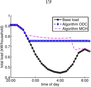
[image:31.612.246.394.140.255.2]

Base load Algorithm ODC Algorithm MCH

Figure 2.4: All EVs plug in at 20:00 with deadline at 9:00 on the next day, and need to charge 10kWh electricity. Multiple purple dash-dot curves correspond to the total load profiles in different iterations of Algorithm MCH.

Homogeneous case Although Algorithm ODC obtains optimal charging profiles irrespective of the EV specifications, we simulate the homogeneous case to compare it against Algorithm MCH. In this example, all EVs plug in at 20:00 with deadline at 9:00 the next morning, and need to charge 10kWh electricity. Figure 2.4 shows the average total load profiles per household in each iteration of Algorithm ODC and MCH. Both algorithms converge to a valley-filling profile. Moreover, Algorithm ODC converges with a single iteration.

20:00 0:00 4:00 8:00

0.4 0.5 0.6 0.7 0.8 0.9 1

time of day

[image:31.612.246.394.455.569.2]

Figure 2.5: All EVs plug in at 20:00 with deadline at 9:00 on the next day, but need to charge different amounts of electricity that is uniformly distributed between 0 and 20kWh.

(32)

20:00 0:00 4:00 8:00 0.4

0.5 0.6 0.7 0.8 0.9 1

time of day

[image:32.612.246.393.57.197.2]

Figure 2.6: All EVs need to charge 10kWh electricity, but plug in at different times (uniformly distributed between 20:00 and 23:00) with different deadlines (uniformly distributed between 6:00 to 9:00 on the next day).

Different plug-in times and deadlines Figure 2.6 shows the average total load profiles per household at convergence of Algorithm ODC and MCH in another non-homogeneous case, where EVs plug in at different times with different deadlines. Algorithm ODC still converges to a valley-filling profile in a few iterations, while Algorithm MCH converges to a total load profile that is significantly lower around 6:00 to 9:00. This is because Algorithm MCH uses a penalty term to limit the deviation of the individual EV charging profiles from the average charging profile. EVs plug in at different times with different deadlines, but are forced to follow the same charging profile. Algorithm ODC changes the “deviation from the average penalty” to the “deviation from the previous iteration penalty”. While preserving convergence, Algorithm ODC no longer imposes different EVs to follow a common average charging profile, therefore successfully deals with the heterogeneity in charging deadlines. In fact, Theorem 2.8 implies that Algorithm ODC always obtains optimal charging profiles, even if the EVs plug in at different times, have different deadlines, charge different amounts of electricity, and have different maximum charging rates.

2.5 Conclusions

(33)

Chapter 3

Real-Time Distributed Load

Control

Real-time load control has the potential to compensate for the random fluctuations of renewable generation, by reducing or shifting the power consumption of electric loads in response to generation fluctuations. In this chapter, a real-time distributed algorithm that schedules deferrable loads to reduce the deviation of aggregate load (load minus renewable generation) from some externally specified target is proposed. At every time step, the algorithm minimizes the expected deviation to go with updated predictions on renewable generation and deferrable load arrivals. We prove that suboptimality of the algorithm vanishes quickly as prediction horizon expands. Further, we evaluate the algorithm via trace-based simulations.

Literature A number of distributed deferrable load control algorithms have been proposed in the literature. Some of these algorithms are evaluated based on simulations [4,55,77], while some others have theoretical performance guarantees [41, 75]. In particular, the algorithm proposed in [75] is optimal if electric vehicles are identical, and the algorithm proposed in [41] achieves optimality even if electric vehicles are not identical.

However, the algorithms proposed in [4, 41, 55, 75, 77] do not consider the uncertainties in renew-able generation and deferrrenew-able load arrivals. In practice, only predictions of these quantities are known ahead of time, and the impact of prediction errors can be dramatic, e.g., see Figure 3.3.

Algorithms that consider the uncertainties in renewable generation or/and deferrable load arrivals have also been proposed in the literature. Most of these algorithms are evaluated with simulation-based studies, e.g., [22,31,34], while some are provided with analytic performance guarantees [28,72, 97]. For example, the algorithm proposed in [28] proposes an algorithm that achieves the optimal competitive ratio in the case where renewable generation is precisely known (and constant). The algorithm proposed in [72] also has certain worst-case performance guarantees.

(34)

chapter focuses on the “average-case” perspective to highlight the value of prediction.

Summary The goal of this chapter is to propose a retime distributed deferrable load control al-gorithm that incorporates uncertain predictions on deferrable load arrivals and renewable generation. In particular, contributions of the chapter are threefold.

First, wemodel renewable generation prediction evolution as a Wiener filtering process[106] (see Section 3.1.1), that is able to model any zero-mean and stationary prediction error.

Second, wepropose a real-time distributed algorithm (Algorithm 2) for deferrable load control in the presence of uncertainties (in Section 3.2), that reduces the deviation of aggregate load (load minus renewable generation) from some externally specified target profile. At every time step, Algorithm 2 minimizes the expected deviation to go with up-to-date predictions on deferrable load arrivals and renewable generation. A key technique is the introduction of apseudo load, that is simulated at the centralized coordinator to represent future deferrable load arrivals.

Third, weanalyze the expected deviation achieved by Algorithm 2 and provide trace-based simu-lations. In particular, the theorems in Section 3.3 characterize the impact of prediction inaccuracies on the expected deviation. As time horizon expands, the expected deviation approaches the optimal value (Corollary 3.7), and the performance gain of Algorithm 2 increases over the optimal open-loop control (Corollary 3.10, 3.11). Trace-based simulations in real-world settings are provided in Section 3.4 to validate the analytic results, highlighting that Algorithm 2 obtains a small suboptimality even under high uncertainties, and improves significantly over the optimal open-loop control.

3.1 Model Overview and Notation

This chapter studies the design and analysis of real-time deferrable load control algorithms to com-pensate for the random fluctuations of renewable generation. In the following we present a model for this scenario that includes renewable generation, non-deferrable loads, and deferrable loads, which are described in turn.

Throughout, we consider a discrete-time model over a finite time horizon. The time horizon is divided into T time slots of equal length and indexed 1, . . . , T. In practice, the time horizon could be one day and the length of a time slot could be 10 minutes.

3.1.1 Renewable Generation and Non-Deferrable Load

We aggregate renewable generation and non-deferrable load into a single process, termed thebase load b = _{b(τ)_}T

(35)

Figure 3.1: Diagram of the notation and structure of the model for base load, i.e., non-deferrable load minus renewable generation.

To model the uncertainty of base load, we use a causal filter based model described as follows, and illustrated in Figure 3.1. In particular, the base load at timeτis modeled as a random deviation

δb=_{δb(τ)_}T

τ=1 around its expectation ¯b={¯b(τ)}Tτ=1. The process ¯b is specified externally to the model, e.g., from historical data and weather report, and the processδb(τ) is further modeled as an uncorrelated sequence of identically distributed random variables e={e(τ)}T

τ=1 with mean 0 and varianceσ2_{, passing through a causal filter. Specifically, let} _f ₌_{_f₍_τ₎_}∞

τ=−∞ denote the impulse

response of this causal filter and assume thatf(0) = 1, thenf(τ) = 0 forτ <0 and

δb(τ) =

T X

s=1

e(s)f(τ−s), τ= 1, . . . , T.

Given the model above, at timet= 1, . . . , T, a prediction algorithm can estimate the sequencee(s) fors= 1, . . . , t, and predictsbas1

bt(τ) = ¯b(τ) + t X

s=1

e(s)f(τ₋s), τ = 1, . . . , T. (3.1)

Note thatbt(τ) =b(τ) forτ= 1, . . . , tsincef is causal.

This model allows for non-stationary base load through the specification of ¯band a broad class of models for uncertainty in the base load viaf and e. In particular, two specific filtersf that we consider in detail later in the paper are:

Example 3.1. A filter with finite but flat impulse response, i.e., there exists ∆∈(0, T) such that

f(t) =

    

1 if 0_≤t <∆ 0 otherwise;

Example 3.2. A filter with an infinite and exponentially decaying impulse response, i.e., there exists

a_∈(0,1) such that

f(t) =

    

(36)

These two filters provide simple but informative examples for our discussion in Section 3.3.

3.1.2 Deferrable Load

To model deferrable loads we consider a setting wherendeferrable loads arrive over the time horizon, each requiring a certain amount of electricity by a given deadline. Further, a real-time algorithm has imperfect information about the arrival times and sizes of these deferrable loads.

More specifically, we assume a total of n deferrable loads and label them in increasing order of their arrival times by 1, . . . , n, i.e., load i arrives no later than load i+ 1 for i = 1, . . . , n₋1. Further, letn(t) denote the number of loads that arrive before (or at) timet for t= 1, . . . , T and fixn(0) := 0. Thus, load 1, . . . , n(t) arrive before or at timetfort= 1, . . . , T andn(T) =n.

For each deferrable load, its arrival time and deadline, as well as other constraints on its power consumption, are captured via upper and lower bounds on its possible power consumption during each time. Specifically, the power consumption of deferrable loadiat timet,pi(t), must be between

given lower and upper boundsp_i(t) andpi(t), i.e.,

p_i(t)≤pi(t)≤pi(t), i= 1, . . . , n, t= 1, . . . , T. (3.2)

These are specified externally to the model. For example, if an electric vehicle plugs in with Level II charging then its power consumption must be within [0,3.3]kW. However, if it is not plugged in (has either not arrived yet or has already departed) then its power consumption is 0kW, i.e., within [0,0]kW. Further, we assume that a deferrable load i must withdraw a fixed amount of energyPi

by its deadline, i.e.,

T X

t=1

pi(t) =Pi, i= 1, . . . , n. (3.3)

Finally, thendeferrable loads arrive randomly throughout the time horizon. Define

a(t) :=

n(t)

X

i=n(t−1)+1

Pi (3.4)

as the total energy request of all deferrable loads that arrive at timetfort= 1, . . . , T. We assume that _{a(t)_}T

t=1 is a sequence of independent identically distributed random variables with mean λ and variances2_{. Further, let}

A(t) :=

T X

τ=t+1

a(τ) (3.5)

denote the total energy requested after timetfort= 1, . . . , T.

(37)

deferrable load total energy requestE(A(t)). However, a real-time algorithm has no other knowledge about deferrable loads that arrive after timet.

3.1.3 The Deferrable Load Control Problem

Recall that the objective of real-time deferrable load control is to compensate for the random fluc-tuations in renewable generation and non-deferrable load in order to “flatten” the aggregate load

p0={p0(t)}Tt=1, which is defined as

p0(t) =b(t) +

n X

i=1

pi(t), t= 1, . . . , T. (3.6)

In this chapter, we focus on minimizing thevariance of the aggregate loadp0,V(p0), as a measure of “flatness”, that is defined as

V(p0) = 1

T

T X

t=1

p0(t)−_T1 T X

τ=1

p0(τ)

!2

. (3.7)

To summarize, the optimal deferrable load control (ODLC) problem is as follows. Let T :=

{1, . . . , T}, N :={0, . . . , n}, and defineN+_:=_{N \{}₀_}_.

ODLC: min

T X

t=1

p0(t)−_T1 T X

τ=1

p0(τ)

!2

over pi(t), i∈ N, t∈ T

s.t. p0(t) =b(t) +

n X

i=1

pi(t), t∈ T; (3.8a)

p_i(t)_≤pi(t)≤pi(t), i∈ N, t∈ T; (3.8b) T

X

t=1

pi(t) =Pi, i∈ N. (3.8c)

In the above ODLC problem (3.8), the objective is simplyT times the variance of aggregate load,

V(p0), and the constraints correspond to equations (3.6), (3.2), and (3.3), respectively. We chose

(38)

3.2 Algorithm Design

Given the optimal deferrable load control (ODLC) problem defined in (3.8), the first contribution of this chapter is to design an algorithm that solves the ODLC problem in real-time, given uncertain predictions of base load and deferrable loads.

There are two key challenges for the algorithm design. First, the algorithm has access only to uncertain predictions at any given time, i.e., at time t the algorithm only knows deferrable loads 1 to n(t) rather than 1 to n, and only knows the prediction bt instead of b itself. Second, even

if there were no uncertainty in predictions, solving the ODLC problem (3.8) requires significant computational effort when there are a large number of deferrable loads.

Motivated by these challenges, in this section we design a distributed algorithm that provides strong performance guarantees even when there are uncertainties in the predictions. The algorithm we propose is built on Algorithm 1 in Chapter 2, which is distributed but assumes exact knowledge (certainty) about base load and deferrable loads.

In this section, we adapt Algorithm 1 to the setting where there is uncertainty in base load and deferrable load predictions, while maintaining strong performance guarantees. In particular, in this section we assume that at timet, only the predictionbt is known, notbitself, and only information

about deferrable loads 1 ton(t) and the expectation of future energy requests E(A(t)) are known. Algorithm statement: To adapt Algorithm 1 to deal with uncertainty, we replace the base loadb by its predictionbt in Algorithm 1.

However, dealing with the unavailability of future deferrable load information is trickier. To do this we use a pseudo deferrable load, which is simulated at the coordinator, to represent future deferrable loads. At each timet, we will predict the electricity demandpn+1(τ) of future deferrable

loads at timesτ=t+ 1, . . . , T, and denote these forecasts bypn+1:={pn+1(τ)|τ =t, . . . , T}with

pn+1(t) := 0. As will be seen in Algorithm 2, these forecast are chosen at each time tto minimize

the`2 norm of aggregate load, subject to the following (and other) constraints:

T X

τ=t

pn+1(τ) =E(A(t)). (3.9)

We also assume thatpn+1 is point-wise upper and lower bounded by some upper and lower bounds

pn+1 andp_n₊₁, i.e.,

p_n₊₁(τ)≤pn+1(τ)≤pn+1(τ), τ =t, . . . , T. (3.10)

Note thatp_n₊₁(t) =pn+1(t) = 0. The boundsp_n₊₁ andpn+1 should be set according to historical data. Here, for simplicity, we consider them to bep_n₊₁(τ) = 0 andpn+1(τ) =∞forτ =t+1, . . . , T. Given the above setup, the coordinator solves the following ODLC(t) problem at every time slot

(39)

and define_N+₍_t_{) :=}

N(t)_\{0_}fort= 1,2, . . . , T. Let_T(t) :=_{t, t+ 1, . . . , T_} fort= 1,2, . . . , T.

ODLC(t) : min X

τ∈T(t)

p0(τ)₋ 1

T−t+ 1

T X

s=t

p0(s)

!2

over pi(τ), i∈ N(t)∪ {n+ 1}, τ ∈ T(t);

s.t. p0(τ) =bt(τ) + n(t)

X

i=1

pi(τ) +pn+1(τ), τ∈ T(t); (3.11a)

p_i(τ)_≤pi(τ)≤pi(τ), i∈ N+(t)∪ {n+ 1}, τ ∈ T(t); (3.11b) X

τ∈T(t)

pi(τ) =Pi(t), i∈ N+(t)∪ {n+ 1} (3.11c)

where Pi(t) = Pi−Pτt−=11pi(τ) is the energy to be consumed at or after timet fori = 1, . . . , n(t);

andPn+1(t) =E(A(t)) is the expected future energy request.

Now, adjusting Algorithm 1 to solve ODLC(t) gives Algorithm 2, which is a real-time, shrinking-horizon control algorithm. Note that if base load prediction is exact (i.e., bt =b fort = 1, . . . , T)

(40)

Algorithm 2Deferrable load control with uncertainty

Input: At time t, the coordinator knows the prediction bt of base load and the number n(t) of

deferrable loads. Each deferrable load i _{∈ N}+₍_t_{) knows its future energy request} _P

i(t) and

power consumption bounds (pi, p_i). The utility sets stopping criteria.

Output: At timet, each deferrable loadi∈ N+₍_t_{) computes its own}_{_p

i(τ)}Tτ=t.

At time slott= 1, . . . , T:

1: each old deferrable load i ∈ N+₍_t₋_{1) initializes its schedule} _{_p(0)

i (τ)}Tτ=t as the schedule it

computes at time slot t−1; each new deferrable load i∈ N+₍_t₎

\N+₍_t

−1) initializes its schedule{p(0)i (τ)}Tτ=tas

p(0)i (τ)←0, τ∈ T(t);

2: k←0;

3: the coordinator computes pseudo loadp(_nk₊₁) as

p(nk+1) ← argmin

X

τ∈T(t)

 bt(τ) +

n(t)

X

i=1

p(ik)(τ) +pn+1(τ)  

2

(3.12)

s.t. p_n₊₁(τ)≤pn+1(τ)≤pn+1(τ), τ∈ T(t);

X

τ∈T(t)

pn+1(τ) =Pn+1(t);

the coordinator then calculates control signalc(k)_as

c(k)(τ)← _n1₍_t₎p(0k)= 1

n(t)

 bt(τ) +

n(t)

X

i=1

p(ik)(τ) +p

(k)

n+1(τ)



, τ∈ T(t);

4: ifk≥1 andkc(k)−c(k−1)k ≤, the coordinator broadcasts a stopping signal to go to Step 7); otherwise the coordinator broadcastsc(k)_{to deferrable load}_i

∈ N+₍_t_);

5: each deferrable load i∈ N+(t) calculates a new charging profile{p_i(k+1)(τ)}T_τ₌_tas

p(_ik+1) _← argmin X

τ∈T(t)

c(k)(τ)pi(τ) +

1 2

X

τ∈T(t)

pi(τ)−p(ik)(τ) 2

(3.13)

s.t. p_i(τ)_≤pi(τ)≤pi(τ), τ∈ T(t); X

τ∈T(t)

pi(τ) =Pi(t)

and sends_{pk_i+1(τ)_}T

τ=tto the coordinator;

6: k←k+ 1; go to Step 3);

Distributed Load Control in Multiphase Radial Networks

Distributed Load Control in Multiphase Radial Networks

Lingwen Gan

Acknowledgements

Abstract

Contents

List of Figures

List of Tables

Chapter 1

Introduction

1.1

Distributed Load Control

1.2

Optimal Power Flow

1.3

Thesis Overview

Chapter 2

Distributed Load Control

2.1

Problem Formulation

2.2

Optimal Charging Profile

2.3

Distributed Scheduling Algorithm

2.3.1

The Optimal Distributed Charging Algorithm

2.4

Case Studies

2.5

Conclusions

Chapter 3

Real-Time Distributed Load

Control

3.1

Model Overview and Notation

3.1.1

Renewable Generation and Non-Deferrable Load

3.1.2

Deferrable Load

3.1.3

The Deferrable Load Control Problem

3.2

Algorithm Design