Exploring Moore space filling geometry for compact filter realization

EXPLORING MOORE SPACE-FILLING GEOMETRY FOR COMPACT FILTER REALIZATION

EZRI MOHD

A project report submitted as partial fulfilment of the requirements for the award of

Degree of Master of Electrical Engineering

Faculty of Electrical and Electronic Engineering Universiti Tun Hussein Onn Malaysia

ACKNOWLEDGEMENT

, Praise to The Almighty Allah, finally with His limitless kindness for granting me a healthy and strength to complete this work at last. For my beloved mother and father, my wife and sons for supporting me during my study.

The author would like to express his sincere appreciation to his supervisor, Prof. Madya Dr. Samsul Haimi bin Dahlan for the support given throughout the duration for this project.

ABSTRACT

A compact RF filter is desirable in modern wireless communication system. The Moore curves fill the defined space and compact the effective geometry within the same line length. The miniaturization rate of the planar microstrip filter can be accomplished by applying the Moore curves with defined iteration and yet still maintaining the acceptable performance. In this work, the 2nd _{iterated Moore curves} bandpass filter is designed to operate at center frequency, fcenter= 2.45GHz on

ABSTRAK

TABLE OF CONTENTS

TITLE i

DECLARATION ii

ACKNOWLEDGEMENT iii

ABSTRACT iv

ABSTRAK v

TABLE OF CONTENTS vi

LIST OF TABLES ix

LIST OF FIGURES x

LIST OF SYMBOLS AND ABBREVIATIONS xiv

LIST OF APPENDICES xvi

LIST OF PUBLICATIONS xvii

CHAPTER 1 INTRODUCTION 1

1.1 Overview 1

1.2 Problem Statement 2

1.3 Objectives of the Project 2

1.4 Scope of the Project 3

1.5 Outline of the Report 4

CHAPTER 2 LITERATURE REVIEW 6

2.1 Introduction 6

2.2 Background of Fractal Geometry 6

2.3 RF Filter’s terminology 8

2.3.1 Bandpass definition 8

2.3.2 Selectivity 10

2.3.3 Quality factor, Q 11

2.4 Moore Fractal Resonator 12

2.5 Review of Fractal Resonator 13

2.5.2 Hilbert Resonator 16

2.6 Coupling Coefficient of Coupled Line 17

2.6.1 Input and Output Coupling 17

2.6.2 Adjacent Resonator’s coupling 19

2.7 Class of Coupling 21

2.8 Review of Microwave Fractal Filter 22

2.9 Defected ground structure DGS 25

2.10 Conclusion 27

CHAPTER 3 METHODOLOGY 28

3.1 Introduction 28

3.2 Design and development study 28

3.3 Simulation 32

3.4 Fabrication 34

3.5 Measurement 36

CHAPTER 4 DEVELOPMENT OF MOORE FRACTAL RESONATOR 38

4.1 Design of Moore Fractal Resonator 38

4.2 Resonator’s dimension 38

4.3 Performances of Moore Resonator 40

4.4 Parametric Studies of Moore Resonator 42

4.5 Measurement of Moore Resonator 44

4.6 Conclusion 47

CHAPTER 5 DEVELOPMENT OF MOORE BANDPASS FILTER 48

5.1 Design Approach 48

5.1.1 Topology of Coupled Moore Resonator 48

5.1.2 Technique of Feeding 50

5.2 Parametric Studies on geometry’s dimension 51

5.2.2 Distance gap between Moore resonators elements,g_spacing 55 5.3 Moore Filter design at center frequency,

center

f = 2.45GHz 60

5.3.1 Optimized dimension of designed

Moore fractal filter 60

5.3.2 Transmission Response 61

5.3.3 Surface current density 63

5.4 Comparison with Parallel-Coupled

Line Filter 64

5.5 Moore Filter with DGS 66

5.6 Realization of Moore bandpass filter 70

5.6.1 Fabrication 70

5.6.2 Measurement 70

CHAPTER 6 CONCLUSION AND RECOMMENDATION 73

6.1 Conclusion 73

6.2 Recommendation 75

REFERENCES 76

LIST OF TABLES

1.1 Scope of the proposed Moore filter 4

2.1 Fractal applications in different fields 8

2.2 Requirement of modern RF bandpass filter 8

4.1 Comparison of resonator’s size 40

4.2 Transmission characteristics of modelled resonators 41

4.3 Relation between resonant frequency and value of gap,g and width,w 43

4.4 Transmission characteristics of measured resonators 45

5.1 Transmission characteristic associated to variation of x and w 51

5.2 Validation of equation 5.1 between calculation and simulation 53

5.3 Validation of equation 5.2 between calculation and simulation 55

5.4 Summary of passband region attributes 62

5.5 Comparison of passband attributes 65

5.6 Simulated frequency suppression with different length of DGS transverse slot, s 68

5.7 Summary of comparison between measurement and simulation 72

LIST OF FIGURES

2.1 Examples of fractal geometries 7 2.2 Transmission coefficient, S₂₁of bandpass filter 9 2.3 Symmetrical response of bandpass filter 11 2.4 (a) Moore curves and (b) Hilbert curves with

2nd _{iteration level (n=2) 12}

2.5 Square dual-mode resonator with Minkowski’s iteration [8] 14

2.6 Relationship between L and g at 14GHz and transmission characteristic for 1st _iteration square Minkowski resonators. [8] 14

2.7 Transmission characteristics of square, 1st _and 2nd _{iteration Minkowski resonators. [8] 15}

2.8 Transmission characteristics of 2nd _square Minkowski resonators. [8] 15 2.9 Open line λ/2 resonator to Hilbert fractal

curves. [8] 16

2.10 Transmission characteristics of Hilbert

Resonator. [8] 16

2.11 Types of coupling between resonators 17 2.12 Method used to determine the unloaded

quality factor 18 2.13 Reference plane added to RLC equivalent

circuit. [9] 19 2.14 response with input/output are weakly

coupled [8] 20 2.15 Class of coupling between resonators. [8] 22 2.16 Transmission zero and selectivity 22 2.17 (a) 2nd _{iteration and (b) 3}rd _{iteration of Hilbert}

2.18 3rd _{order meandered line with (a) magnetic} coupling and (b) electrical coupling and

their transmission responses [11] 24

2.19 3rd _{order Hilbert filter with (a) magnetic} coupling and (b) electrical coupling and their transmission responses. [11] 24

2.20 (a) 2nd and (b) 3rd iteration of Moore fractal and their transmission responses. [12] 25

2.21 (a) 3-Dimensional view of the DGS unit section. (b) The newly proposed equivalent circuit. [14] 26

3.1 Process flow of the project 39

3.2 Mesh solver and adaptive mesh refinement setting 33

3.3 Boundary conditions setting 33

3.4 Flow chart of fabrication process using photolithography technique 34

3.5 Laminator machine 35

3.6 UV exposure machine 35

3.7 The measurement outcome of network analyzer 37

3.8 Measurement setup to excite both ports of Moore resonator 37

4.1 Evolution of Moore fractal 38

4.2 Geometry of designed resonators, (a) half-wavelength resonator, (b) 1st _iteration Moore, (c) 2nd _{iteration Moore. 39}

4.3 Transmission characteristic of modelled resonators 40

4.4 Gap and width of Moore resonator 42

4.5 Transmission response with gap variation [w=2.5mm] 43

4.6 Resonant frequency with gap variation [w=2.5mm] 43

4.8 Realization of the resonators, (a) half-wavelength resonator, (b) 1st _iteration Moore, (c) 2nd _{iteration Moore 45} 4.9 Comparison between simulation and

measurement of λ/2 line resonator 46 4.10 Comparison between simulation and

measurement of 1st _{iteration Moore resonator 46} 4.11 Comparison between simulation and

measurement of 2nd _{iteration Moore resonator 47} 5.1 Optimized dimension of Moore resonator

element 48 5.2 Proposed topologies of the filter 49

5.3 Transmission characteristic S₂₁ for electric and

magnetic coupling 49

5.4 Input/output feeding technique 50 5.5 Transmission response of Moore filter with

tapping and mutual coupling feedlines 50 5.6 Relation between center frequency,

center

f

5.7 S21 response with different width of fractal at center frequency,

f

5.8 Distance spacing, g_spacing between Moore

resonators with magnetic coupling 56

5.9 Coupling coefficient, k associated with distance spacing, g_spacing 56

5.10 Transmission response, S₂₁ associated with variation of distance spacing, g_spacing 57 5.11 Extremely over-coupled with distance gap,

spacing

g = 0.1mm 58

5.12 Over-coupled with distance gap,

spacing

5.13 Under-coupled with distance gap,

spacing

g = 2.0mm and 4.0mm 59

5.14 Optimized dimension of designed Moore filter 60 5.15 Transmission response of designed Moore filter 61 5.16 Bandpass response of designed Moore filter 61 5.17 Simulated surface current at 2.45GHz

(passband region) 63 5.18 Simulated surface current at 2.8GHz

(reject band region) 64

5.19 Conventional 6th _{order parallel coupled line}

bandpass filter 64

5.20 Comparison of passband characteristic between Moore filter and parallel coupled

line filter 65

5.21 The dumbbell DGS at the Moore I/O feedlines 67

5.22 Transmission response with different length of DGS transverse slot, s 67

5.23 Relation between frequency suppression and length of DGS transverse slot, s 68 5.24 Moore bandpass filter with dumbbell DGS 69 5.25 Transmission response of Moore bandpass

filter with DGS 69 5.26 The fabricated Moore bandpass filter 70 5.27 Comparison between simulated and

measured result of the proposed filter

(full observed range) 71

5.28 Comparison between simulated and measured result of the proposed filter

LIST OF SYMBOLS AND ABBREVIATIONS

r

ε

eff

ε - Effective dielectric constant

AR

L - Maximum passband ripple

λ - Wavelength of the radio wave

c

f - Resonant frequency

center

f - Center frequency of the filter

H

f - Upper frequency at -3dB below from insertion loss

L

f - Lower frequency at -3dB below from insertion loss

f

∆ - Different between two split peak frequency

out

P - Output power from filter

in

P - Input power to filter

Q - Quality factor

e

Q - External quality factor

L

Q - Loaded quality factor

U

Q - Unloaded quality factor

n

n

S - Total perimeter length of Moore fractal with n-iteration

L - Length of outer area side Moore fractal

w - Width of fractal

g - Gap spacing between Moore segments

spacing

g - Gap spacing between two coupled Moore resonators

x - Length of Moore open line segment

k - Coupling coefficient

11

S - Reflection coefficient

21

o

Z - Characteristic impedance BW - Bandwidth of bandpass filter I/O - Input and output

UV - Ultra-violet RF - Radio frequency

LIST OF APPENDICES

APPENDIX TITLE PAGE

A Published Paper 79 B Moore BPF with upper cavity: A brief study 87 C Datasheet: RT/duroid®_{5870/5880 by Rogers}

Corporation 88 D Datasheet: Bandpass Cavity Filter SF24251 by

LIST OF PUBLICATIONS

Journal:

(i) Mohd, E. & Dahlan, S. H. (2017). Miniaturization of Resonator based on Moore Fractal. TELKOMNIKA (Telecommunication, Computing, Electronics and Control), Universitas Ahmad Dahlan (UAD), Vol.13,

CHAPTER 1

INTRODUCTION

1.1 Overview

In a front-end receiver of microwave communication systems, RF filter is an essential component. The filters are designed to pass specific frequency within a particular passband and reject the other frequency outside the operating frequency band. Nowadays, the bandpass filter with high performance, compact size and low cost is desired to enhance the overall performance of communication system. The well-known planar structure filter such as microstrip is already in small size but there are needs to reduce the size of a particular application especially in portable communication devices.

Currently, the miniaturization of microwave filter focuses on a planar filter structure. Open line resonator filter is a famous filter structure that had been widely studied and commercialized. Parallel coupled line and hairpin resonator are preferred for passband application and can frequently be found inside communication devices. These structures are simple to design and the bandwidth can be controlled with ease. As further development, they are benefited from its flexibility to fold the resonator as a result of more compact form.

higher order of filter could be designed by iterative construction while the overall physical realization is miniaturized.

The high dielectric constant substrate is used to miniaturize microstrip filter and a variable geometry of filters is required. Hence, numbers of new filter configuration can be modelled possibly. However, dissipation losses correlated with the size of the filter and it affect the performance of the filter overall. The parametric study will be conducted to define ‘trade-off’ between the technical performance and miniaturization based on application.

1.1 Problem Statement

With rapid demand for smaller and reliable wireless communication system, RF devices miniaturization become the research trend. A new filter circuit design which suits the manufacturing ability and cost yet still maintaining the required performance is developed.

The parallel coupled line resonator is popular for designing the narrowband filter and widely used for many years since 1958. However, there are disadvantages of this filter although it requires simple design and supports a wide range of fractional bandwidth from 5% to 50%. The length of coupled line resonator is too long and increases directly proportional to the order of the filter. The hairpin line filter is developed based on parallel coupled line filter with folding the λ/2 resonator structure. Recently, the microstrip fractal geometry had become a trend in designing planar structure on RF devices such as antenna and filter. The Moore fractal has several unique criteria such as essential dual properties, space curve filling and self-similarity which is the iteration can be done in a defined space. Theoretically, this feature will enable the miniaturization of the filter. In this thesis, by applying Moore fractal construction, a compact bandpass filter applicable for wireless application in ISM band is modelled, designed and validated.

1.1 Objectives of the Project

agreement. In this work, the miniaturization is expected to be achieved by using high permittivity material, RT/duroid®_{5880 and fractal configuration with its variation of} resonant structure. The configuration of parallel coupled line filter is designed and its physical realization are observed as well as filter’s performance to be compared with designed Moore fractal filter.

The challenging task is to design a bandpass filter with lowest possible insertion loss while miniaturizing the filter and keeping the low coupling between resonators. Some parameters highly correlated to each other and achieve one requirement may reduce the other one. Hence, analysis and parametric study of the trend is presented in this work. To achieve the aim, the objectives of the study are: (i) To design a compact bandpass filter using Moore fractal at ISM band. (ii) To analyze the performance of Moore fractal filter in term of geometry and

technical aspect.

(iii) To explore the correlation between variations of Moore geometry with electrical performance of the Moore BPF.

(iv) To prototype a Moore BPF and validate experimentally.

1.2 Scope of the Project

A compact resonator filter is achieved by using a Moore fractal structure. A reduction in the form factor is made by folding the resonator line while maintaining its length approximately and is represented in term of iteration. The iterative construction of the fractal Moore filter geometry is limited up to the second iteration. This designed filter is compared with conventional parallel coupled line. The scope of this work are:

(i) Design and fabricate a microstrip 2nd _{order of bandpass Moore fractal filter at} center frequency of 2.45GHz with a narrowband response based on electrical and material specifications as shown in Table 1.1.

(iii) The optimized design of the Moore BPF should consider the accuracy of in-house fabrication which is set up to 0.5mm precision to guarantee the desired geometry.

(iv) The resulted correlation between geometry’s dimensions and the transmission characteristic of the designed Moore BPF are valid for a defined range of width of fractal, w and center frequency, only.

(v) The simulated results are verified experimentally in a typical laboratory environment without any special shielding and setup by using a calibrated network analyzer that able to sweep for a range of frequency from 500MHz to 10GHz.

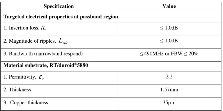
Table 1.1: Specification of the proposed Moore filter

Specification Value

Targeted electrical properties at passband region

1. Insertion loss, IL ≤ 1.0dB

2. Magnitude of ripples, L_AR ≤ 1.0dB

3. Bandwidth (narrowband respond) ≤ 490MHz or FBW ≤ 20%

Material substrate, RT/duroid®₅₈₈₀

1. Permittivity,

ε

2. Thickness 1.57mm

3. Copper thickness 35µm

1.5 Outline of the Report

This report consists of six chapters. Chapter 1 presented the overview of the project and its objectives. The scope limitations of the works are also described briefly in this chapter.

Chapter 2 presented the literature review by discussing general knowledge of microstrip fractal and its associated characteristics. The evolution of conventional microstrip transmission line to Moore resonator fractals are explained. The main filter characteristics that define the performance of the filter such as selectivity and coupling technique are discussed. Then, the advantages and limitations of other fractal resonators and filters by other researchers are reviewed.

Chapter 3 explained the methodology of the project to accomplish the objectives with a scope above. The approach starts with the development of single element of Moore resonator through simulation and realization to validate the potential as a filter. With a verified result from Moore resonator, the Moore bandpass filter is designed. This chapter also describes the simulation procedure and fabrication technique.

Chapter 4 described the first stage of this project by presenting a resulted preliminary study of Moore resonator by simulation and experiment. This study also involved the comparison between different iteration of Moore fractals and their performances. The correlation between Moore geometries and transmission characteristics is reviewed.

Chapter 5 focused on developing the ultimate goal of this project which is designing a Moore bandpass filter. In this chapter, the variation of technique to excite the filter through different class coupling and feedline are explained. The outcomes of parametric studies and the resulted correlation between different parameters with transmission characteristic are discussed. This chapter also revealed the control parameters of the Moore fractal geometry to achieve specific filtering criteria.

CHAPTER 2

LITERATURE REVIEW

2.1 Introduction

Chapter 2 discussed the general background of microwave fractal filter based on planar microstrip technology. The suitability of Moore fractal curve to be used as a microstrip microwave bandpass filter is explored. Studies are done based on knowledge on planar coupled mode microstrip since the fractal curve will have many adjacent microstrip structures on completed filter’s geometry and induced a coupling effect. Coupling between microstrip coupled line is one of the elements that made a microwave filtering’s effect. Besides, reviews about other previous studies on microwave resonator or filter based on fractal curves are discussed. Some fractal design consideration and transmission characteristics are compared. At the end of this chapter, the advantages and limitation of the microwave fractal filters which are done by previous researchers will be summarized.

2.2 Background of Fractal Geometry

There are many types of fractal iteration that had been introduced as early as 1870s. The simplest structure to describe the fractal iteration is Cantor. The Cantor set give us an early idea about fractal iteration and consists a set points lying on a single line segment. The Cantor iteration has infinite numbers and self-similarity properties. Others types of fractal geometry are Peano, Hilbert, Sierpinski, Von Koch and Moore in Figure 2.1. From visual observation, one should notify that these curves are actually repeating themselves in fractional dimension with finite occupied area.

Figure 2.1: Examples of fractal geometries

Nowadays, fractals are implemented in many fields due to their main properties; self-similarity and space filling. In microwave field, fractal have been used to develop compact RF devices, most notably antennas and filters. Some of these applications are summarized in Table 2.1.

(a) Cantor line (b) Peano curve (c) Hilbert curve

Table 2.1: Fractal applications in different fields.

Field Application

Statistical Probability theory called statistical fractal to predict extreme/catastrophic

events.

Chemistry Research structural design and optimized design of microfluidic and

nanofluidic devices for mixing, reaction and heat transfer.

Acoustics Invention of a revolutionary type of acoustic barrier of soundproof walls.

Cosmology Understanding the distribution of luminous matter in the universe.

Computer Science Apply degree of recursion and self-similarity at different scales in creating

an animation or to compress lossy image.

Electromagnetic Miniaturization of RF devices and performance enhancement such as

selective frequency and harmonic suppression. [3]

2.3 RF Filter’s terminology

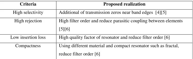
In order to produce high performance of the filter, there are main criteria that the filter must be able to fulfill. Table 2.2 concludes the general need and the proposed realization.

Table 2.2: Requirement of modern RF bandpass filter

Criteria Proposed realization

High selectivity Additional of transmission zeros near band edges [4][5]

High rejection High filter order and reduce parasitic coupling between elements

[5][6]

Low insertion loss High quality factor of resonator and reduce filter order [6]

Compactness Using different material and compact resonator such as fractal,

reduce filter order [6]

2.3.1 Bandpass definition

dual-band of bandpass filter. The characteristic response of passband filter also should be considered prior to its application.

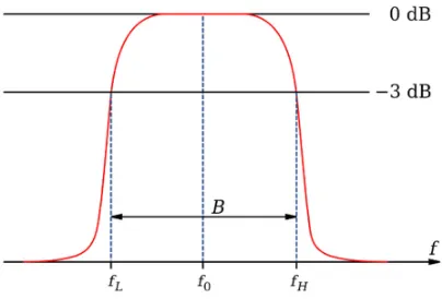
When designing a bandpass filter, we must determine the level of rejection or attenuation that must be achieved by the filter at frequencies outside of its passband bandwidth. The bandwidth is associated with cut-off frequencies upper and lower of filter’s center frequency at -3dB from maximum insertion loss in passband region. Figure 2.2 illustrated the terminology to express the bandwidth of passband filter.

Figure 2.2: Transmission coefficient, S₂₁of bandpass filter

The bandwidth is calculated by subtracting the lower frequency, f_Lwhere the response attenuates by 3dB from the higher frequency, f_Hwith same attenuation level as equation 2.1.

BW = f_H − f_L (2.1) The bandwidth of the filter can be categorized as narrowband or wideband. It depend on the range of the passband region and the suitability based on application. Generally, the category of the filter is determined by fractional bandwidth, FBW in percentage.

Fractional bandwidth, FBW = *100

center

f BW

(2.2)

magnitude decibel (dB). Insertion loss is an indicator of forward transmission gain of 2-port network system.

Insertion loss, IL_dB =

in out

P P 10

log

10 (2.3)

To realize the definition of filtering characteristics for RF system, the device

must be able to attenuate 50% of the input power in stopband region. Calculate using

the formulation of insertion loss, IL_dBwould be approximately -3.01dB. Theoretically, the low insertion loss in passband region is desired due to zero loss in

allowing all the input power and high insertion loss as possible as can be is desired

in stopband region.

2.3.2 Selectivity

Selection of proper RF filter for a certain application is determined by its selectivity.

Selectivity is described as the level of attenuation at some frequencies that is rejected

from passband region of the filter. It usually is represented by a slope which indicate

how many decibel drop from cut-off frequency in both lower and upper side. For an

example, the cavity resonator at 155MHz has a selectivity which can be described as

15dB drop at interval of 1MHz in both lower and upper cut-off frequencies.

Normally, the transmission coefficient of RF bandpass filter is not

symmetrical. The response may be described of having 5dB drop at interval 1MHz

at lower side of center frequency and 10dB at upper side. This condition indicated

that the filter has a better selectivity at upper side of center frequency. The Chebyshev

response has a better selectivity than Butterworth response which is indicated by a

sharp slope, while quasi-elliptic response usually has an equal selectivity in both side

from center frequency.

The selectivity of the filter can be improved by using a quasi-elliptic response

[4]. Quasi-elliptic response has transmission zeros in both side of center frequency.

Figure 2.17 illustrates the importance of having symmetrical response with

occurrences of finite transmission zeros. The writers proposed a source load coupling

to realize quadrupled in second order filter in order to create two finite transmission

Figure 2.3: Symmetrical response of bandpass filter [4]

2.3.3 Quality factor, Q

High performance of the filter generally achieve high value of quality factor. The Q

factor can described as a unit less ratio of the total energy stored in the lumped

element of the resonator (inductor and capacitor) to the dissipated power in the

resistor. As we may recalled, the microstrip microwave resonator can be represented

by an equivalent lumped elements circuit. However the extraction of the accurate

lumped elements of the filter always become a great challenges to the researchers

especially when dealing with complex structural like fractal geometry.

There are two ways to extract the quality factor of resonator; equivalent of

lumped elements circuit and transmission type measurement [7]. Since in this work

implement the Moore fractal, the latter method of extraction is reviewed in section

2.5.1 later on.

2.4 Moore Fractal Resonator

Microwave resonators that are designed using planar technologies such as microstrip

can be compacted by adopting the fractal construction. Recently, researchers are

exploring the fractal construction in order to meet the needs of smaller antennas and

filters with reduced cost.

The Moore fractal curve is a continual line that is folded several times in term

of iteration. Moore fractal begin with a single line and has a special recursive

SFC make a miniaturization on RF devices is possible. Hilbert and Moore curve are

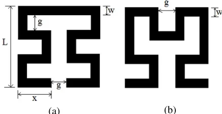
outlined in Figure 2.4. The main different is the endpoints of these fractal, Moore has

its endpoint coincides with each other and create a spacing gap. From microstrip

technology’s perspective, a gap between microstip lines creates a capacitance which

influences the coupling characteristic.

Figure 2.4:(a) Moore curves and (b) Hilbert curves with 2nd _{iteration level( = 2).}

The total perimeter length, S of Moore fractal is determined by with n is the iteration level.

S_n

(

)

1 2 1 1 2       − + +

= (2.4)

L is the length of outer area side Moore fractal and determined the area occupied by fractal curve. From study, the total length of line segment is longer from

its origin but the physical area is miniaturized. To develop a resonator using Moore

fractal, the single resonator with certain length is folded to some iteration.

Theoretically, the total length is maintained to resonate it to the same frequency for

different iteration. However, the length need to be optimized in physical realization

to achieve same resonant frequency for a half wavelength resonator, first iteration

and second iteration respectively.

Ideally, the designer would prefer to fit resonator in the small area as much

as possible by increasing the iteration level of Moore curve. As for microstrip, the

width, w and the gap space between, g are the parameters needed to be defined to model a Moore curve. It depends on the iteration level, n. A higher iteration Moore

curve would decrease the resonator width, w and spacing between lines, g to fit the

total perimeter length, S curves in the smaller area. The relation between dimensions as depicted by:

L=2n*

(

)

The external side, L could be controlled by defining the width of the resonator, w and spacing between lines, g. However, from the study the other external side, x would be varying to resonate the structure to a specific frequency for second

iteration ( = 2) and is defined as an optimization technique.

A smaller width of resonator, w would increase the dissipation losses, thus the quality factor, Q should diminishes. So, the designer should consider this parameter if the application emphasize on higher quality factor, Q and at the same

time, miniaturization is required. The trade-off between miniaturization and

dissipation losses should be defined well according to priority.

2.5 Review of Fractal Resonator

This section discussed about studies that had been done on microwave resonators.

The studies reveals the suitability and potential of two types of resonators for

compacted RF devices and filters based on Minkowski and Hilbert fractal curves. [8]

2.5.1 Minkowski Resonator

The square dual-mode resonator is designed to be operated at center frequency,

14GHz. As depicted in Figure 2.5, the iteration of Minkowski fractal can be done by

removing several small square or rectangular repeatedly. The iteration techniques can

be done in two methods; square iteration or rectangular iteration. The designer should

Figure 2.5: Square dual-mode resonator with Minkowski’s iteration [8]

We should notice that the value of L is preserved while the value of g

decreases after each iteration. After an infinite number of iterations, we should expect

that there is no more left as the iteration has consumed the space square.

For a dual mode resonator to be operated at a specific frequency is determined

by the value of L and g. The writers concluded the relationship between L and g to maintain a resonant frequency at 14GHz and some cases to validate the transmission

characteristics in Figure 2.6.

Figure 2.6: Relationship between L and g at 14GHz and transmission characteristic for 1st _{iteration square Minkowski resonators. [8]}

With same resonant frequency at 14GHz, the rate of miniaturization can be

controlled by the value of g. This is a definite conclusion that the Minkowski iteration is capable of producing a smaller square dual-mode resonator. In term of transmission

characteristics, the first spurious frequency which is twice resonant frequency occurs

the highest frequency and the writers concluded the miniaturization also could

improve the spurious response.

Further investigation, Minkowski with 2nd _{iteration resonator had been}

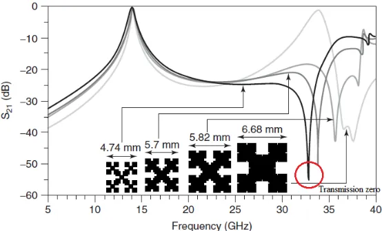
developed to observe the transmission characteristics. Figure 2.7 shows the

comparison of the square resonator with 1st _{and 2}nd _{Minkowski’s iteration. The first}

spurious frequency is attenuated significantly in higher iteration and in addition to

that, also produce the transmission zero characteristics. The writers also designed

four different sizes of 2nd _{Minkowski’s iteration to examine the transmission}

characteristics and the result is depicted in Figure 2.8. The smaller size of the

resonator with same Minkowski’s iteration would also provide a better spurious

response.

Figure 2.7: Transmission characteristics of square, 1st _{and 2}nd _{iteration Minkowski}

resonators.[8]

2.5.2 Hilbert Resonator

The Hilbert fractal curve is constructed by folding a single open line resonator to ‘U’

shape and is iterated by a special curves. The iteration can be done by repeated

folding again and again into finite space with infinite length. A λ/2 open line

resonator is folded according to Hilbert’s curve up to 2nd _{Hilbert’s iteration as in}

Figure 2.9. All the resonators are designed with respective dimension to have same

resonant frequency at 9.78GHz.

From transmission characteristics as illustrated in Figure 2.9, we noticed that

open line resonator and ‘U’ shape resonator have a spurious response at twice the

resonant frequency. The 1st _{iteration Hilbert had a spurious frequency slightly above}

twice the resonant frequency and produced transmission zeros response. The 2nd

iteration Hilbert also had a spurious frequency above twice the resonant frequency

and the transmission zero is apparently moved closer to the resonant frequency. This

response suggested an improvement in selectivity.

Figure 2.9: Open line λ/2 resonator to Hilbert fractal curves. [8]

As a conclusion, the fractal resonator especially Minkowski and Hilbert tend

to suggest that the higher iteration number, the miniaturization factor should be

increased. The performances with better selectivity due to the occurrence of

transmission zero and harmonic suppression is possible.

2.6 Coupling Coefficient of Coupled Line

Proximity between two or more transmission line introduces coupling effect through

their fringing fields respectively. This coupling effect could be desirable or

undesirable. In printed circuit board, the coupling effect is undesirable as it cause a

crosstalk, but in microwave devices such as directional coupler, it is desirable. The

coupling between transmission lines enable power transfers between lines at the

resonant frequency.

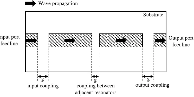
For a microstrip transmission lines, there are two types of coupling, input or

output coupling and coupling between adjacent resonators as illustrated in Figure

2.11. Both characterize the excitation between the resonators.

Figure 2.11:Types of coupling between resonators

2.6.1 Input and Output Coupling

The input coupling characteristic depends on the spacing gap, g between the first

resonator and input feedline and output coupling depends on the spacing between last Wave propagation

Substrate

Input port feedline

Output port feedline

g _g g

coupling between adjacent resonators

resonator and output feedline. From reflection coefficient transmission characteristic,

, we could calculate the input coupling by measuring its resonant frequency,

and bandwidth corresponding to 180 phase shift from resonant frequency. Then, the

input coupling is represented by external quality, factor given by:

f f Q_e

∆

= 0 _(2.6)

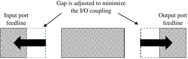
Since the performance of filter is referred to unloaded quality factor, ,

spacing gap between input or output feedlines can be manipulated. To eliminate the

effect of input and output coupling, the spacing between feedlines and resonators is

adjusted until attenuation, transmission characteristic at least 20dB from its

maximum value at resonant frequency as depicted in Figure 2.11. The 3dB bandwidth

is measured to calculate unloaded quality factor, by extrapolating external quality

factor, given by

) (

1 _{21 o}

e f S Q Qu −

= (2.7)

Higher quality factor suggests more power is delivered between resonator lines due

to strong coupling between resonators.

Figure 2.12:Method used to determine the unloaded quality factor.

2.6.2 Adjacent Resonator’s coupling

Coupling between adjacent resonators determine the maximum power transfer at

certain resonant frequency. A good filter resonate at designed resonant frequency.

Variation in spacing gap between resonator elements shift the resonant frequency.

When the spacing between resonators is shorter, the resonant frequency will be Output port

feedline Input port

feedline

decreases. These assumption has been used to optimize the modelled design in order

to achieve desired operating frequency of planar resonator.

As suggested by Y. Hongyu [9], the calculation methods of coupling

coefficient between resonators are presented. When two resonators are located in

close proximity, two modes of couplings are existed; electric coupling and magnetic

coupling. The electric coupling creates capacitance effect while the magnetic

coupling introduces inductance effect as showed in equation (1) in this paper. From

the general coupling coefficient equation, the researchers propose three methods in

order to calculate the coupling coefficient more accurately based on certain

conditions.

One of the methods is to add an electric and magnetic wall between coupled

resonators. This is done by adding a reference plane in the middle of RLC equivalent

circuit as illustrated in Figure 2.13.

Figure 2.13: Reference plane added to RLC equivalent circuit. [9]

In this method, the coupling coefficient is calculated in term of electrically or

magnetic coupling only. The electric coupling is calculated by short-circuiting the

reference plane (T-T’ plane) to create an electric wall while the magnetic wall is

created by open-circuiting the plane. Then the resonant frequency based on additional

of electric/magnetic wall is calculated respectively. Coupling coefficient for both

capacitance and inductance coupling can be found by knowing the value of resonant

frequency in both modes. Below equation summarize the method:

(i) Coupling coefficient for capacitance coupling (electric coupling),

_{2 2} 2 2 e m e m m f f f f C C k + − =

= (2.8)

(ii) Coupling coefficient for inductance coupling (magnetic coupling), _{2 2} 2 2 m e m e m f f f f L L k + − =

= (2.9)

From this equation, we should expect that if coupling coefficient polarity is negative,

then we can conclude that the resonators are magnetically coupled and otherwise.

Coupling coefficient also can determined with S-parameter method

introduced by P. Jarry and J. Beneat [8]. This method require the gap adjustment

between input/output feedline and the resonators. To define the resonator coupling

coefficient, the input/output couplings need to be coupled weakly in order to prevent

any interference with coupling between resonators. Attenuation of at least 10dB

between two weakly coupled resonant frequencies and is assumed to make sure

the interference do not occurred as depicted in Figure 2.14.

Figure 2.14: response with input/output are weakly coupled. [8]

Then, the coupling coefficient, k between resonators can be calculated by:

₂ 1 2 2 2 1 2 2 f f f f k + −

= (2.10)

This method applies to both electric and magnetic coupling. Farid Ghanem, Tayeb

A. Denidni and Renato-G Bosisio presented the same method to calculate the

coupling coefficient, k for planar cross-coupled resonator filters with electric or magnetic coupling and mixed coupling [13]. The result revealed that the dimension

exhibit desired response. They also explained the application of equation (2.10) in

comprehensive graphical representation.

2.7 Class of Coupling

For a periodic structure, the arrangement of planar resonator determines the class of

coupling either electrical or magnetic coupling. In electrical coupling, an electrical

field is concentrated inside coupling area or sometimes is referred as positive

coupling. In other hand, a magnetic coupling has its electrical field is concentrated

outside the coupling area. Hence, it is opposite with electrical coupling and known

as negative coupling. The term positive and negative can be seen in phase

characteristic as it is opposite to each other. We can observe that with same distance

of the gap between resonators but a different class of coupling, magnetic coupling

provide stronger coupling. The orientation of the resonators may introduce mixed

coupling too. This method can be used as a mechanism to control the bandwidth of

the filter (narrowband or wideband).

Depending on the application, transmission zero also sometimes is desirable

in filter design. Transmission zero often relates to the ability of the filter to reject the

unwanted frequency in the stop-band region. Interestingly, we can control the

occurrence of transmission zero by electrical or magnetic coupling. Electrical

coupling creates transmission zero at low pass section whereas magnetic coupling

influences transmission zero at high pass section. Besides that, it also helps to

attenuate or eliminate the spurious frequency and enhance band-stop rejection as well

Figure 2.15:Class of coupling between resonators. [8]

Figure 2.16:Transmission zero and selectivity

2.8 Review of Microwave Fractal Filter

There are many research on microwave filter based on fractal geometry. This section

will review some techniques and result. As fractal geometries have two common

properties, self-similarity and space-filling, the designer has an option to investigate

different fractal geometries.

Microstrip bandpass filter based on Hilbert fractal geometry of 2nd _{and 3}rd

iteration are designed by Y.S. Mezaal [10]. The Hilbert fractal geometry is designed

from conventional half-wavelength resonator filter and considerable miniaturization

is achieved. Two structures of Hilbert fractal are coupled electrically to create a

In term of performance, the filter produces transmission zero at both low and high

pass region at least -50dB ( response). The 3rd _{iteration of Hilbert fractal produce}

better transmission response with symmetrical transmission zero around resonant

frequency. This result suggest better band-stop rejection and improve selectivity.

However, the width trace become smaller (w = 0.22mm) and need precision value

during fabrication. With smaller trace width, dissipation losses is higher and the

tradeoff between miniaturization rate and performance should be a concern. Hence,

this technique might not suitable to be used if fabrication is done in general printing

circuit board (university) which is not specialized in microwave.

Figure 2.17:(a) 2nd _{iteration, (b) 3}rd _{iteration of Hilbert filters and its transmission}

response [10]

To further improve the miniaturization, P. Jarry, J. Beneat and E. Kerherve

implemented the pseudo-elliptic response [11]. For the same selectivity, this

approach allows further reduction in size and the construction will be simplified by

using lower order of the filter. Meandered line, Hilbert and dual-mode Minkowski

bandpass filter are designed and compared. 3rd _{order meandered line and Hilbert}

fractal are fabricated and experimental results are presented. Interestingly, they also

re-arranged the structures to demonstrate magnetic and electrical coupling. From

both experimental results, it suggests that class of coupling will determine the

location of transmission zero either in left (electrical coupling) or right (magnetic

coupling). This information is useful for the designer to decide where they would

and selectivity. In this paper, all the input and output feedline is excited by mutual

coupling.

Figure 2.18:3rd _{order meandered line with (a) magnetic coupling, (b)}

electrical coupling and their transmission responses [11]

Figure 2.19:3rd _{order Hilbert filter with (a) magnetic coupling, (b) electrical}

coupling and their transmission responses [11] (a)

(b)

REFERENCES

1. Mandelbrot, B. B. (1983). The Fractal Geometry of Nature. New York: W.

H. Freeman.

2. Falconer, K. (2003). Fractal Geometry: Mathematical Foundations and Applications. West Sussex: John Wiley & Sons Ltd.

3. Krzysztofik, W. J. (2017). Fractals in Antennas and Metamaterials Applications, Fractal Analysis - Applications in Physics, Engineering and Technology, Dr. Fernando Brambila (Ed.), InTech,

4. Kolmakov, Y. A., Savino, A. M. & Vendik, I. B. (2004). Quasi-elliptic two

pole microstrip filter. 15th _{International Conference on Microwaves, Radar}

and Wireless Communications (IEEE Cat. No.04EX824), pp. 159-161 Vol.1. 5. Liu, H., Ren, B., Hu, S., Guan, X., Wen, P., & Tang, J. (2017). High-Order

Dual-Band Superconducting Bandpass Filter With Controllable Bandwidths

and Multitransmission Zeros. IEEE Transactions on Microwave Theory and

Techniques, vol. 65, no. 10, pp. 3813-3823.

6. Hsieh, L. H. & Chang, K. (2003). Compact, low insertion-loss,

sharp-rejection, and wide-band microstrip bandpass filters. IEEE Transactions on Microwave Theory and Techniques, vol. 51, no. 4, pp. 1241-1246.

7. Behagi, A. A. (2015). RF and Microwave Circuit Design: A Design Approach Using (ADS).Ladera Ranch, California: Techno Search.

8. Jarry, P. & Beneat, J. (2009). Design and Realizations of Miniaturized Fractal Microwave and RF Filters. New Jersey: A John Wiley & Sons.

9. Hongyu, Y. (2012). The calculation methods of coupling coefficient between

resonators. 10th International Symposium on Antennas, Propagation & EM

Theory (ISAPE2012), Xian, pp. 741-743

10. Mezaal, Y. S. (2009). A New Microstrip Bandpass Filter Design Based on

Hilbert Fractal Geometry for Modern Wireless Communication Applications.

11. Jarry, P., Beneat, J. & Kerherve, E. (2010).Fractal microwave filters. 2010 IEEE 11th Annual Wireless and Microwave Technology Conference (WAMICON), Melbourne, FL, pp. 1-5.

12. Mezaal, Y. S., Ali, J. K. & Eyyuboglu, H. T. (2015). Miniaturised microstrip

bandpass filter based on Moore fractal geometry. International Journal of Electronics, Vol.102, No. 8, pp. 1306-1319.

13. Ghanem, F., Denidni, T. A. & Bosisio, R. G. (2003). Design of miniaturized

planar cross-coupled resonator filters. Microwave and Optical Technology

Letters, Vol. 36, No. 5, pp. 406-411.

14. Park, J. S., Kim, J. H., Lee, J. H., Kim, S. H. & Myung, S. H. (2002). A novel

equivalent circuit and modeling method for defected ground structure and its

application to optimization of a DGS lowpass filter. 2002 IEEE MTT-S International Microwave Symposium Digest (Cat. No.02CH37278), vol.1,

Seattle, WA, USA, pp. 417-420.

15. Khandelwal, M. K., Kanaujia, B. K. & Kumar, S. (2017). Defected Ground

Structure: Fundamentals, Analysis, and Applications in Modern Wireless

Trends. International Journal of Antennas and Propagation 2017, Article ID 2018527, 22 pages.

16. Ferh, A. E., & Jleed, H. (2014). Design, simulate and approximate parallel

coupled microstrip bandpass filter at 2.4 GHz. 2014 World Congress on

Computer Applications and Information Systems (WCCAIS), Hammamet, pp. 1-5.

17. Bhattacharjee, S., Poddar, D., Mukherjee, S., Saurabh, S. & Das, S. (2013).

Design of Microstrip Parallel Coupled Band Pass Filter for Global Positioning

System. Journal of Engineering, Computers & Applied Sciences (JEC&AS),

Vol.2, No.5, pp. 28-32.

18. Hanna, E., Jarry, P., Kerherve, E. & Pham, J. M. (2006). A novel compact

dual-mode bandpass filter using fractal shaped resonators. 2006 13th IEEE International Conference on Electronics, Circuits and Systems, Nice. pp. 343-346.

19. Chakravorty, P., Das, S., Mandal, D. & Lanjewar R. (2015). Feed Line

20. Ahn, D., Park, J. S. & Kim, C. S. (2001). A Design of the Low-Pass Filter

Using the Novel Microstrip Defected Ground Structure. IEEE Transactions on Microwave Theory and Techniques, vol. 49, no. 1, pp. 86-93.

21. Han-Jan Chen, H. J., Huang, T. H., Chang, C. S., Chen, L. S., Wang, N. F.,

Wang, Y. H. & Houng, M. P. (2006). A novel cross-shape DGS applied to

design ultra-wide stopband low-pass filters. IEEE Microwave and Wireless Components Letters, vol. 16, no. 5, pp. 252-254.

22. Barra, M., Collado, C., Mateu, J, & O'Callaghan, J. M. (2005).

Miniaturization of superconducting filters using Hilbert fractal curves. IEEE Transactions on Applied Superconductivity, vol. 15, no. 3, pp. 3841-3846.

23. Namsang, A., & Akkaraekthalin, P. (2008).Microstrip bandpass filters using

asymmetrical tapered-line resonators for improved stopband characteristics.

2008 International Conference on Microwave and Millimeter Wave Technology, Nanjing, 2008, pp. 2-5.

24. Mezaal, Y. S., Eyyuboglu, H. T. & Ali, J. K. (2014). New Microstrip

Bandpass Filter Designs Based on Stepped Impedance Hilbert Fractal

Resonators. IETE Journal of Research, Vol.60, No.3, pp. 257-264.

25. Lahmissi, A. & Challal, M. (2017). Microstrip dual-band bandpass filter

design using folded coupled lines. 2017 5th International Conference on

Electrical Engineering - Boumerdes (ICEE-B), Boumerdes, Algeria, pp. 1-4. 26. Pozar, D. M. (2012). Microwave Engineering 4th _{Edition. Danvers, MA: John}

Wiley & Sons, Inc.

27. Hong, J. S. & Lancaster M. J. (2001). Microstrip Filters for RF/Microwave Applications. New York: John Wiley & Sons, Inc.

28. Swanson, D. & Macchiarella, G. (2007). Microwave filter design by synthesis