Convolutional Neural Network Architecture Study for Aerial Visual Localization

(1)

Air Force Institute of Technology

AFIT Scholar

Theses and Dissertations Student Graduate Works

3-22-2019

Convolutional Neural Network Architecture Study

for Aerial Visual Localization

Jedediah M. Berhold

Follow this and additional works at:https://scholar.afit.edu/etd

Part of theNavigation, Guidance, Control and Dynamics Commons, and theSystems and Communications Commons

This Thesis is brought to you for free and open access by the Student Graduate Works at AFIT Scholar. It has been accepted for inclusion in Theses and Recommended Citation

Berhold, Jedediah M., "Convolutional Neural Network Architecture Study for Aerial Visual Localization" (2019).Theses and Dissertations. 2246.

(2)

CONVOLUTIONAL NEURAL NETWORK ARCHITECTURE STUDY FOR AERIAL

VISUAL LOCALIZATION

THESIS

Jedediah Mark Berhold, Captain, USAF AFIT-ENG-MS-19-M-010

DEPARTMENT OF THE AIR FORCE AIR UNIVERSITY

AIR FORCE INSTITUTE OF TECHNOLOGY

Wright-Patterson Air Force Base, Ohio DISTRIBUTION STATEMENT A

(3)

The views expressed in this document are those of the author and do not reflect the official policy or position of the United States Air Force, the United States Department of Defense or the United States Government. This material is declared a work of the U.S. Government and is not subject to copyright protection in the United States.

(4)

AFIT-ENG-MS-19-M-010

CONVOLUTIONAL NEURAL NETWORK ARCHITECTURE STUDY FOR AERIAL VISUAL LOCALIZATION

THESIS

Presented to the Faculty

Department of Electrical and Computer Engineering Graduate School of Engineering and Management

Air Force Institute of Technology Air University

Air Education and Training Command in Partial Fulfillment of the Requirements for the Degree of Master of Science in Electrical Engineering

Jedediah Mark Berhold, B.S.E.E. Captain, USAF

March 21, 2019

DISTRIBUTION STATEMENT A

(5)

THESIS

Jedediah Mark Berhold, B.S.E.E. Captain, USAF Committee Membership: Dr. Robert C. Leishman, PhD Chair Dr. John F. Raquet, PhD Member Dr. Donald T. Venable, PhD Member

(6)

Abstract

In unmanned aerial navigation the ability to determine the aircrafts’s location is essential for safe flight. The Global Positioning System (GPS) is the default modern application used for geospatial location determination. GPS is extremely robust, very accurate, and has essentially solved aerial localization. Unfortunately, the signals from all Global Navigation Satellite Systems (GNSS) to include GPS can be jammed or spoofed. To this response it is essential to develop alternative systems that could be used to supplement navigation systems, in the event of a lost GNSS signal.

Public and governmental satellites have provided large amounts of high-resolution satellite imagery. These could be exploited through machine learning to aid onboard navigation equipment to provide a geospatial location solution. Deep learning and Convolutional Neural Networks (CNNs) have provided significant advances in specific image processing algorithms.

This thesis will discuss the performance of CNN architectures with various hyper-parameters and industry leading model designs to address visual aerial localization. The localization algorithm is trained and tested through satellite imagery of a local-ized area of 150 square kilometers. Three hyper-parameters of focus are: initializa-tions, optimizers, and finishing layers. The five model architectures are: MobileNet V2, Inception V3, ResNet 50, Xception, and DenseNet 201.

The hyper-parameter analysis demonstrates that specific initializations, optimiza-tions and finishing layers can have significant effects on the training of a CNN architec-ture for this specific task. The lessons learned from the hyper-parameter analysis were implemented into the CNN comparison study. After all the models were trained for 150 epochs they were evaluated on the test set. The Xception model with pretrained

(7)

initialization outperformed all other models with a Root Mean Squared (RMS) error of only 85 meters.

(8)

Acknowledgements

To my wonderful wife and children:

Thank you for all the support, love, and encouragement.

(9)

List of Figures

Figure Page

1 Aircraft body frame. . . 20

2 WGS84, ECEF and NED coordinate systems . . . 21

3 Convolutional layers . . . 25

4 MobileNet V2 Inverted Residual Bottleneck . . . 36

5 Inception Modules . . . 42

6 Residual Connection . . . 43

7 Inception-ResNet Introduction Layers . . . 43

8 Inception-ResNet Modules . . . 44

9 Inception-ResNet Architecture . . . 44

10 Xception Design Structure . . . 45

11 DenseNet Dense Block . . . 45

12 Unformatted Satellite Imagery . . . 47

13 Formatting Imagery for Data Processing . . . 50

14 Experimental Network Layout . . . 56

15 Relationship between initializers, optimizers and finishing layers . . . 57

16 Training Dataset Coordinate Locations . . . 64

17 Test Dataset Coordinate Locations . . . 64

18 Hyper-parameter: Optimizers’ Training/Validation over Epochs . . . 67

19 Hyper-parameter: Optimizers’ Validation Minus Training over Epochs . . . 67

20 Hyper-parameter: Optimizers’ Validation Minus Training Violin Plot . . . 68

(13)

Figure Page 21 Hyper-parameter: Finishing Layers’

Training/Validation over Epochs . . . 70 22 Hyper-parameter: Finishing Layers’ Validation Minus

Training over Epochs . . . 70 23 Hyper-parameter: Finishing Layers’ Validation Minus

Training Violin Plot . . . 71 24 Hyper-parameter: Initializers’ Training/Validation over

Epochs . . . 72 25 Hyper-parameter: Weight Initializers’ Validation Minus

Training over Epochs . . . 72 26 Hyper-parameter: Weight Initializers’ Validation Minus

Training Violin Plot . . . 73 27 Hyper-parameter: Default Model vs Super Model

Training/Validation over 150 Epochs . . . 74 28 Hyper-parameter: Default Model vs Super Model

Validation Minus Training over Epochs . . . 74 29 Hyper-parameter: Default Model vs Super Model

Validation Minus Training Violin Plot . . . 75 30 RMS Prediction Error for Hyper-Parameter Comparison . . . 76 31 RMS Prediction Error Optimizer Comparison . . . 77 32 Optimizer Models’ Highest Prediction Error Geographic

Distribution . . . 77 33 Optimizer Models’ Lowest Prediction Error Geographic

Distribution . . . 78 34 RMS Prediction Error Finishing Layer Comparison . . . 79 35 Finishing Layer Models’ Highest Prediction Error

Geographic Distribution . . . 79 36 Finish Layer Models’ Lowest Prediction Error

(14)

Figure Page 38 Initializer Models’ Highest Prediction Error Geographic

Distribution . . . 80

39 Initializer Models’ Lowest Prediction Error Geographic Distribution . . . 81

40 RMS Prediction Error Initializer Comparison . . . 82

41 Hyper-parameter Comparison Default Model Worst Error Images . . . 82

42 Hyper-parameter Comparison Super-Model Worst Error Images . . . 83

43 Model Comparison Training/Validation over 150 Epochs . . . 84

44 Model Comparison Training/Validation over 150 Epochs . . . 85

45 Model Comparison Validation Minus Training Violin Plot . . . 86

46 Model Comparison Imagenet Initializer Test Set Violin Plot . . . 87

47 Model Comparison Untrained Initializer Test Set Violin Plot . . . 87

48 Xception Geographic Distribution of Highest Errors . . . 89

49 MobileNet Geographic Distribution of Highest Errors . . . 90

50 Custom Loss Training/Validation over 150 Epochs . . . 100

51 MMSE vs MSE Test Error Violin Plot . . . 101

(15)

List of Tables

Table Page

1 Model Parameters and Batch Size . . . 66 2 Hyper-parameter Test Set Frobenius Norm Error . . . 76 3 Hyper-parameter Super-Model Test Set Frobenius Norm

Error . . . 81 4 Model Comparison Test Set Frobenius Norm Error . . . 88 5 MMSE Loss Test Set RMS Error . . . 101

(16)

List of Abbreviations

Abbreviation Page

ANT Autonomy and Navigation Technology . . . 52

ANN Artificial Neural Network . . . 13

CNN Convolutional Neural Network . . . 63

IMU Inertial Measurement Unit . . . 97

GPU Graphics Processing Unit . . . 63

GNSS Global Navigation Satellite Systems . . . 95

CPU Central Processing Unit . . . 53

BN Batch Normalization . . . 38

VOR Very High Frequency Omni-directional Range . . . 18

EKF Extended Kalman Filter . . . 17

SIFT Scale Invariant Feature Transform . . . 17

NGA National Geospatial Intelligence Agency . . . 20

WGS84 World Geodetic System 1984 . . . 16

GPS Global Positioning System . . . 1

ECEF Earth Centered Earth Fixed . . . 49

NED North East Down . . . 46

UAV Unmanned Aerial Vehicle . . . 49

SGD Stochastic Gradient Descent . . . 29

AdaGrad Adaptive Gradient Algorithm . . . 29

AFRL Air Force Research Laboratory . . . 48

AWS Amazon Web Services . . . 65

AI Artificial Intelligence . . . 53

MSE Mean Squared Error . . . 92

MAE Mean Absolute Error . . . 85

MMSE Minimum Mean Squared Error . . . 92

MMAE Minimum Mean Absolute Error . . . 97

RNN Recurrent Neural Network . . . 96

(17)

I. Introduction

Aerial visual localization was the first avigation method used in manned flight[1]. Since that time a more accurate and dependable localization tools have been devel-oped, to include the state of the art GNSS, which have furthered the development of unmanned avigation systems. It is possible for adversaries to jam or deny GNSS sig-nals, presenting a renewed need for visual localization in unmanned flight. This thesis evaluates CNN models, that have recently revolutionized image processing in general, as a novel solution to conduct aerial visual localization. Multiple CNN parameters and model architectures will be analyzed on a dataset designed for this task.

This thesis is organized as follows: Chapter I provides a brief overview and ob-jectives this research is attempting to solve. Chapter II goes into the advances of visual avigation, the coordinate systems, and the hyper-parameters and architec-ture advancements for CNNs. Chapter III discusses the processes used to built the dataset, the system and CNN model architecture, and the methodology to evaluate performance. Chapter IV provides the results of a model hyper-parameter study, and CNN architecture comparison. Finally, ChapterV discusses the conclusions drawn and future improvements to this approach for aerial visual localization.

1.1 Problem Background

(18)

now have unmanned flight where aircraft navigate without the assistant of pilots using signals from space through GNSS. Unfortunately, GNSS signals can be denied[2]. Visual avigation is part of a solution that could aid the aircraft through a signal disruption environment. In unmanned avigation, if signals cannot be properly sent and received from the aircraft, visual localization must be done algorithmically on-board.

Visual odometry is an effective way to detect changes in position and location. Effective algorithms have been developed by the authors of [3, 4, 5, 6, 7, 8, 9, 10, 11, 12]. Visual odometry Artificial Neural Network (ANN) solutions have been developed by the authors of [13, 14, 15, 16, 17, 18] With odometry solutions, errors will exist and slowly perpetuate over time, leading to a lack of global consistency in the position and orientation estimates. The focus of this research is to address these errors though a visual localization CNN.

CNNs are a subset of ANNs which were developed in 1943, but due to the pro-cessing complexity they had not been used for mainstream image propro-cessing un-til the authors of [19] outperformed all the other image classification algorithms with a CNN model ‘AlexNet’ in the 2012 Imagenet competition. Since that time, significant advances have been developed to further improve the performance of CNNs[20, 21, 22, 23, 24, 25, 26, 27, 20, 28, 29, 30, 31].

Some of the improvements in CNNs stem from the extensive work in hyper-parameter development. Advances in methodologies to improve the way weights are initialized in untrained networks to speed up the learning process and improve gen-eralization were developed in [20, 32, 33, 21]. Model optimizers control the process of weight updates during training, and advances in optimizer improvement are observed in [34, 35, 22, 23]. Finishing layers are trade tools to format the CNN output layers into the prediction layer; various finishing layer techiques are shown in [24, 25, 26, 27].

(19)

With all this work on hyper-parameter development, which hyper-parameters work best for aerial visual localization? This research will perform a study on the affects of these hyper-parameters for this task.

Since ‘AlexNet’[19], the 2012 Imagenet dataset has become the benchmark to test the performance of new CNN architectures. Significant advancements in network size and accuracy have been made in [28, 36, 29, 30, 37, 38, 31]. Can these advancements be leveraged for this aerial visual localization? Which network performs the best for this task? This research will study the training and performance of leading CNN architecture designs for aerial visual localization.

1.2 Research Objectives

This research focuses on the effect of model hyper-parameter and architecture design performance in aerial visual localization. To advance this work, this research attempts to meet the following objectives:

• Establish a reliable dataset to perform side by side model comparisons for visual

aerial localization.

• Analyze various CNN hyper-parameters and their effect on the training and

testing of a model on the dataset.

• Compare the performance of multiple industry-leading CNN model

architec-tures’ in both training and testing on the dataset.

1.3 Limitations and Assumptions

This research is focused on studying the effects of CNN variations on a visual aerial localization dataset. This makes the dataset’s affect on this project paramount. The

(20)

This means that the images are taken around the same time each day. This limits the dataset purely to daytime navigation and excludes more difficult times like dawn and dusk. Sample images had no image enhancement steps, such as contrast adjustment, hue distortion, etc. added. The lack of enhancements could affect the network, by training the model to figure out which satellite took the picture and where the satellite was, as opposed to where the image is in the area of interest. Finally, the satellite coverage over the area of interest is not uniform and there is a higher density of satellite imagery closer to the bounds of the area than in the center.

The dataset limitations were balanced by conducting the training and testing from two separate datasets. This does not remedy the daytime limitation, but a network that trained to figure out the satellite would not be able to translate that skill to the testing dataset. While image enhancement methods could be useful in future iterations, the separate datasets will provide a method to verify the learning of image feature detection. The non-uniform area coverage was accepted as it could tend to pull incorrect network classifications to the extreme values, which could help emphasize the network errors during training.

Additional limitations stem from the CNN itself. While CNN processing has come a long way since the beginning, there remains an extremely high level of processing to train and test the CNN. Consequently, there are major limitations on the input image size. Aerial photography can produce high resolution imagery, and the network operations to process those images would require a massive computing infrastructure. All the models used in this architecture can be run on fairly light-weight systems, but this requires a reduced image size. This research uses a 224×224 ×3 image size. Aerial imagery larger than this would require a prepossessing step to format the image to the correct size.

(21)

II. Background

This chapter provides information and literature that is relevant to various aspects of this thesis. The sections of this chapter are organized as follows: Section one dis-cusses aspects of aerial navigation or avigation[40] with emphasis on visual navigation and GNSS. Section two discusses coordinate systems with emphasis on the World Geodetic System 1984 (WGS84), Earth Centered Earth Fixed (ECEF), and North East Down (NED). Section 2.3 discusses deep learning with emphasis on ANN, CNN, and advances in CNN design. Sections 2.4 through 2.7 go into further depth on CNN design. Section 2.4 discusses network weight initializations; 2.5 reviews optimizers; finishing methodologies are described in 2.6, and 2.7 discusses specific benchmark CNN designs.

2.1 Avigation

Aerial navigation, also known as avigation[40], is an expansive and diverse field of study. This section reviews topics pertinent to this study namely visual and satel-lite avigation. Visual avigaton reviews the drawbacks and technological advances in Unmanned Aerial Vehicle (UAV) flight. The GNSS section discusses how satellite systems augment avigation and potential issues.

2.1.1 Visual Avigation

Avigation[40], in the earliest days of flight was essential, but also a challenging problem[1]. Early aviators used basic means, such as a compass, maps, course cal-culators, and sextants[1] to determine the aircraft’s position and direction. These individuals relied on a keen sense of direction and comparing the landmarks they

(22)

eventually supplemented with more advanced instrumentation, such as drift recorders and radio based air position indicators[1], but the ability to identify one’s location based on visual avigation remained essential.

Visual avigation is more than simply looking out the window. Aircrew would use all the tools at their disposal to determine their location. They would integrate compass, horizon and slip gyroscopes, airspeed indicators with visually recognized landmarks[1]. Determining ones position from direction and velocity over time from a known point of departure is known as dead reckoning. Aircrew would depend on dead reckoning to get through segments where it was difficult to visually identify a known landmark such as over oceans, farm fields, or with high cloud cover[40]. Visual avigation was rarely used for extensive navigation without augmentation of instrumentation[1].

Avigation was divided into two parts geo-avigation where one would locate objects viewed outside the aircraft, and aerial astronomy which includes navigating by the stars[40]. This thesis addresses the geo-avigation aspect of visual avigation. This methodology has significant challenges such as darkness and obstruction by clouds, similar landmarks, etc. It is difficult for pilots to visually navigate effectively through these conditions without instrumentation augmentation, and even more challenging to design an automated algorithm to visually navigate.

In modern-day unmanned aviation there have been significant advances in auto-mated visual avigation. Aerial visual odometry, using a monocular camera to detect changes in position and location, algorithms were developed in [3, 41, 6, 7, 9, 10, 11, 12]. The authors in [3, 41, 6] provided attitude and position updates through an Extended Kalman Filter (EKF). Automated visual location identification algorithms were developed in [5, 42]. [5] utilized high resolution satellite imagery to develop a Scale Invariant Feature Transform (SIFT) feature database; then with the Inertial

(23)

Measurement Unit (IMU) and visual inputs determined a correct location rate of 70%[5]. Visual navigation was used in [43, 16] for formation operations. Robust vi-sual systems have been developed for aircraft landing such as [44, 45] which utilizes the optical flow to determine the distance from the ground. Advances in GNSS denied indoor avigation were illustrated in [46, 41, 6, 7, 47].

There has also been some work in visual odometry utilizing ANNs. The authors in [13, 14, 15] used semi-supervised training develop CNN and Recurrent Neural Network (RNN) visual odometry models using a monocular camera dataset. Authors of [48] utilized multiple CNN models to determine a semantic segmentation of the environment, a global pose regression, and two additional models to determine a visual odometry estimation. Authors of [49] utilized RNNs to generate additional map segmentations utilizing imagery. Work has been done by [50] on location identification based off camera images. Additional work in visual odometry using CNNs and RNNs can be found in [16, 17, 18].

2.1.2 Global Navigation Satellite System

GNSS systems are have become essential to aerial localization[51]. GNSS in avi-gation is used for communication, air traffic management, aircraft to aircraft opera-tions in addition to localization[51]. GNSS has enabled a reduction in ground-based navigation aids and aircraft avionics[51]. Prior to GNSS Very High Frequency Omni-directional Range (VOR) stations were placed around the United States for aircraft to triangulate their location. The VOR system is expensive to maintain and is in the process of being decommissioned leaving GNSS to fill in the gaps[52].

Modern GNSS provides much more accurate location information compared to VOR[53]. Unfortunately GNSS and VOR signals can be jammed or spoofed which can deny or provide inaccurate location information[2]. As such an autonomous

(24)

military aircraft must be robust enough to manage a GNSS contested environment.

2.2 Coordinate Systems

Describing the aircraft’s relation with the surrounding world is essential to relate the aircraft’s body frame and the world frame. This thesis will focus on three world frames: the World Geodetic System 1984 (WGS84), the Earth Centered Earth Fixed (ECEF), and the North East Down (NED) coordinate frames. Each one of these coordinate frames has its benefits and drawbacks when relating to the aircraft body frame.

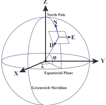
The WGS84 reference frame is a geodetic model used by GPS. WGS84 represents location as the degree offset from the prime meridian, the equatorial plane, and height above sea level, as shown in Figure 2.

Sometimes calculating the world’s shape to determine location can be cumber-some. If so, a geocentric coordinate system, such as ECEF, could be a better fit. ECEF utilizes the center point of the Earth as the origin and establishes the x axis along the prime meridian and equatorial plane. The y axis is 90◦offset from the x

axis also on the equatorial plane, and thez axis is pointing north as seen in Figure 2. The benefit of ECEF is its ability to determine linear distance quickly, and can be useful for satellite and special flight calculations.

When working in a small localized area it may be an adequate to approximate the small segment of the globe as flat, because WGS84, and ECEF make coordinate computations more complex. A localized coordinate system, like NED, could be bet-ter in these circumstances. NED establishes a localized plane tangential to Earth at a specific reference point on the surface of the Earth, as seen in Figure 2. Variability from the globe and NED is negligible for a relatively small region and allows calcula-tions to become more intuitive. NED does not work with large globe seccalcula-tions where

(25)

relative locations can be distorted as a result of the curvature of the Earth.

Figure 1. Aircraft body frame.

2.2.1 World Geodetic System 1984

The National Geospatial Intelligence Agency (NGA) determined a geodetic model of the world to be used in United State’s GNSS system GPS. A previous geodetic model WGS 72 was insufficient in adequately describing the world’s geometry for satellite navigation timing and communication, so the geodetic community came to-gether in the early 1980s to establish WGS84[54]. This update was possible due to extensive altimetry and gravity data from the GRACE satellite mission as well as more accurate geodesy models[54]. The current WGS84 continues to be updated as more precise information is available, and has become the standard reference system due to its accuracy and the global usage of GPS.

The location coordinates in the WGS84 are ellipsoidal. The zero line in the longi-tudinal direction is the Greenwich meridian, and latilongi-tudinal is the Equatorial plane. Longitudinal offsets in Figure 2 are displayed as λ and represent a change in degree

(26)

offsets are displayed as φ, and represent a change in degree in the z direction from

−90◦ to 90◦[55, 56, 57]. WGS84 height variable or h is calculated as the ellipsoidal altitude. A traditional ordering of WGS84 coordinates would be (φ, λ, h).

North Pole Greenwich Meridian

X

Y

Z

Equatorial Plane

λ

φ

N

E

D

Figure 2. Diagram relating WGS84, ECEF and NED coordinate systems and their re-lationships. The graphic represents a simplified version of the WGS84 ellipsoid model. Black arrows are ECEF coordinates, and blue arrows are NED coordinate system cen-tered at a specific location on the Earth.

2.2.2 Earth Centered Earth Fixed

The ECEF coordinate system utilizes geocentric rectangular (Cartesian) coordi-nates (x, y, z) that we learned to love from our mathematics courses[58]. The conver-sion from geodetic to Cartesian coordinates is seen in Equation 1[59].

(27)

X = (RN +h) cosφcosλ Y = (RN +h) cosφsinλ Z = b2 a2RN +h sinφ (1)

In Equation 1, RN is the prime vertical’s radius of curvature and is given in

Equation 2. a is the semi-major axes of the ellipsoid, andb is the semi-minor axes of the ellipsoid. is the eccentricity and it is related to the semi-major and semi-minor axes by Equation 3[59]. RN = a2 p a2_cos2_φ₊_b2_sin2_φ = a p 1−2_sin2_φ (2) 2 = a 2₋_b2 a2 (3)

Conversion from ECEF is slightly more difficult and a concise definition is de-scribed in [58]. ECEF can be an efficient system when calculating orbits, and can be potentially useful when extensive calculations need to occur with respect to a change in an object’s location. ECEF can prove difficult to manage when a localized area is small enough to project it as a flat plane. For this purpose NED would be a better fit.

2.2.3 North East Down

NED is a localized coordinate system used to simplify operations when the working area is sufficiently small that the curvature of Earth is negligible[57]. NED treats the area as a flat plane where the centerpoint of the coordinate system is tangential to the curvature of Earth. This is represented graphically in Figure 2. Thexaxis points

(28)

toward the ellipsoid North, the y axis points to the ellipsoid East, and the z axis points normal to the ellipsoid[56, 57]. The transformation of a point from ECEF to NED is described in Equation 4. (x, y, z)ref,ECEF is the reference point in ECEF

coordinates of the origin or center point of the NED coordinate system; (x, y, z)ECEF

is the location of the point in ECEF coordinates, and RN ED

ECEF is the rotation matrix

from ECEF from to localized NED frame as seen in Figure 5[56].

(x, y, z)N ED =RN EDECEF((x, y, z)ECEF −(x, y, z)ref,ECEF) (4)

RN ED_ECEF =      

−sinφrefcosλref −sinφrefsinλref cosφref

−sinλref cosλref 0

−cosφrefcosλref −cosφref sinλref −sinφref

      (5)

Using the NED coordinate system is especially applicable to smaller UAVs as their field of operation is relatively small when compared to the curvature of Earth[56]. When establishing a NED coordinate system it is important to determine the center reference point properly. Often the takeoff position is selected as the reference point for the NED coordinates[56]. Aircraft heighth is measured in the−z range for NED.

2.3 Deep Learning

The heirarchy of graphs that builds complex concepts out of layering simple ones is deep learning[60]. Deep learning has recently become popular because of its abil-ity to generalize specific problems better than custom designed algorithms[19]. This section will focus on Artificial Neural Networks (ANNs) and more specifically convo-lutional neural networks (CNNs) which are the focus of this thesis. It will describe fundamental aspects of modern CNNs that can be used to tailor networks.

(29)

2.3.1 Artificial Neural Networks

The concept of a neural network has been around since the early days of comput-ing presented by [61] in 1943. These networks borrowed the biological term ’neurons’ to represent weighted activation functions. By connecting a network of these neurons with different weights it was possible to represent specific logic functions. The com-putational ability of the time was not sufficient for complex tasks, yet incremental advancements were made[62, 63, 64, 65]. The modern viability of the neural net-work for image processing came with the success of ‘AlexNet’ in the 2012 ImageNet competition[19]. AlexNet changed image classification standards and created a rush to CNNs as a viable methodology of machine learning.

2.3.2 Convolutional Neural Networks

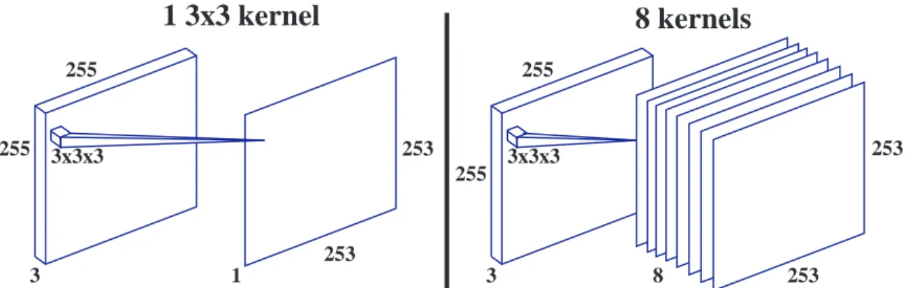
The CNN was first introduced in 1988[66]. CNNs convolve a weighted kernel ma-trix across the input, as seen in Figure 3, as opposed to fully connecting all neurons. This practice afforded the network to work well with images and allowed for pat-tern recognition tasks. Due to the technology of this era computation was difficult for complex networks and CNNs were mostly used for toy problems. A significant advancement came in 1998 with the introduction of gradient descent for network learning by [33]. This provided the basis to update the network and bias weights in a computationally light and effective manner. While CNNs remained computationally heavy at the time, this was a significant advancement in modern CNN training. The attention dedicated to CNNs increased dramatically when [19] outperformed tradi-tional image processing techniques on the ILSVRC-2012 dataset. Since that time many additional developments have occurred to optimize these networks

(30)

1 3x3 kernel

255 255 3 3x3x3 253 253 1

8 kernels

255 255 3 3x3x3 253 251 8 253

Figure 3. The left side is an example of a 3x3 convolution with one filter. The extra dimension on the convolution is the input’s depth. The right side is a 3x3 convolution with 8 filter layers. Note that each filter has individual trainable kernel weights.

2.3.2.1 Further Advances in Convolutional Neural Networks

There are an abundance of techniques that have been used to modify and improve CNNs. A comprehensive overview would span volumes, so only specific items that will be a benefit to later topics will be discussed. First will be techniques to preserve dimensionality and techniques to manage reduction and size manipulation. Next will be methods that manage the way weights are updated and normalized during network training. Finally, an overview of how to combine advanced graph structures into usable outputs is reviewed.

A convolution with a 3x3 kernel size, like that in Figure 3, has an output with a reduced size. This can be useful as the later convolutions require slightly less computations, but can be an obstacle when advanced concatenations are required, such as those in Figure 5. To address this [28, 67, 37, 30] used padding and stride to manipulate the outputs of a convolution layer. ‘Same’ padding refers to adding zeros at the edges of the input matrix to enforce the same dimensions in the output. Padding allows for advanced directed acyclic graphs without specialized operations to retain shapes. Adjusting the convolution stride affords a quick way to cut the output in half. Strides are the steps taken in a convolution between each kernel. A stride

(31)

of one is the traditional convolution that provides the output in Figure 3; a stride of two convolves the kernel with every other member of the matrix. Higher strides are possible, but rarely implemented in practice due to the information loss.

Other network training techniques such as batch normalization and dropout have become a standard in CNNs. Batch normalization as described in [38] is commonplace for CNN architectures [31, 28, 67, 37, 30]. As a network size increases, the effect of weights can saturate the results. Batch normalization is used to reduce this effect in networks. Batch normalization maintains the activation’s mean close to zero and the standard deviation approximately one[38]. Dropout is another technique used to reduce over saturation of specific weights[68]. Dropout takes a certain percentage of the output from the previous layer at random and does not pass those weights to the next layer. This forces the network not to depend on a small number of parameters to make major decisions, but spread the decision making across the network[68].

Performing multiple operations from the same input, or combining results from a previous layer, can add great benefits to a CNN[36, 37]. The question is how to combine them back together? There are two popular methods: addition and concatenation. Addition, as used in [37], requires the dimensions of the two layers to be the same and adds the weights of the two in an output layer with the same dimensionality. Concatenation, as used in [36], allows for one of the dimensions to be different from the others and concatenates across the chosen dimension, which, in practice, is typically the dimensionality of the layers. For example, if the weighted output of layer onex1, with a size of 18×18×4, and layer two x2, with a size of 18×

18×4, the residual addition would be (x1+x2) retaining the original dimensions of the input:18×18×4. Concatenation would result inx1, x2 and expand the dimensionality typically along the last axis; in this case: 18×18×8

(32)

2.4 Initializations

This section discusses methodologies to initialize the various weights for a network. A proper initialization can be taken for granted in CNN infrastructures, but for deep networks they have a significant role to play[32]. A normalized initialization has resulted in reducing the problems of vanishing and exploding gradients[37]. A good initialization can lead to a faster trained network, and some networks need a good initialization to be trained[69]. Advancements in initializers have essentially replaced unsupervised pretraining. A regularizing initializer provides a better baseline for the optimizer and tends to produce improved generalization[32].

Three common initializers are Glorot normal[20], Glorot uniform[20], and orthogonal[20]. Glorot Normal and Glorot Uniform initializers were developed based on best perfor-mance through experimentation and monitoring hidden layer weights[32]. Orthogonal initializers developed in [20] determined a scaled random orthogonal initialization re-duced the issues of exploding and diminishing gradients while providing significant benefits in the learning process[70].

2.4.1 Glorot Normal

The authors in [20] demonstrated that a carefully scaled random initialization exhibits faster convergence than the traditional arbitrary random initialization. This was the formation of Glorot initializations. The method for scaling standard deviation is displayed in (6) where σ is the standard deviation.

σ =

r

2

inputU nits+OutputU nits (6)

This initialization provides a truncated random normal distribution, which is cen-tered on zero, and scaled by the input units and output units of the weight

(33)

ten-sor. While a pretrained initialization still exhibits faster convergence, the Glorot normal exhibits significant convergence for diverse datasets over a random uniform initialization[20].

2.4.2 Glorot Uniform

Prior to carefully scaled initializers, it was commonplace to perform unsupervised pretraining on neural networks to afford state of the art results[20]. Since the advance-ment of second order optimizers and better initializer design, unsupervised pretraining is all but obsolete[69]. Currently the default initializer for untrained convolutional kernels in Keras is the Glorot uniform[71]. The Glorot uniform in Equation 7 il-lustrates the upper and lower bounds to a random distribution which makes up the kernel initialization weights.

±limit=

r

6

inputU nits+OutputU nits (7)

The number of input units and output units in the weight tensor are utilized to scale the limits of this initializer. Glorot initializers work well for many applications, and it has shown superior performance when ReLU activations are used[69].

2.4.3 Orthogonal

In traditional image processing, filters are designed to extract information from the image. Convolutional filter weights in CNNs perform similar tasks once trained. Establishing an orthogonal initialization has the effect of a pass-through filter at an arbitrary orientation. The orthogonal initialization in [20] is explained in Equation 8 where W is the weight matrix and R is an arbitrary orthogonal matrix, M is a diagonal matrix, and Q are eigenvectors of an input output correlation matrix[20].

(34)

W =RM QT (8) Orthogonal initializations lead to productive gradient propagation in deep linear and nonlinear networks. Under the correct conditions, this initialization provides an amplification of the neural activity through the weights, as well as balancing damp-ening activity. As the optimizer back-propagates Jacobians, the Jacobians propagate in a nearly isometric manner[20]. These characteristics are especially beneficial in networks dealing with images such as the ones in this thesis.

2.5 Optimizers

One of the great advances in neural networks was the development of improved optimizers. These were a key part in replacing unsupervised pretraining. Second or-der momentum-based optimizers with carefully scaled initializers have enabled state of the art performance without a pretrained network[20]. These second order opti-mizers use the process of gradient descent, which is a way to minimize an objective (or loss) function of a models parameters by updating in the opposite direction of the loss function gradient with respect to the parameters[72]. The optimizer’s path follows the slope of the loss function surface downhill to a valley[72]. Locating the minimization or maximization requires its parameters to contain a differentiable loss function[22]. Stochastic Gradient Descent (SGD) led to many successes and advance-ments in deep learning. Because loss functions are composed of a sum of subfunctions evaluated at different data subsamples, SGD takes gradient steps down the individ-ual subfunctions[22]. With noisy data, SGD could have a difficult time locating and often overshoots local minimum[22][72]. SGD does not factor the data characteris-tics, which led to the development of Adaptive Gradient Algorithm (AdaGrad)[34]. AdaGrad was designed to incorporate the geometry of data previously observed, thus

(35)

frequently observed data has a lower learning rate than infrequent data with a higher rate[34]. Unfortunately, AdaGrad produced diminishing learning rates. Three opti-mizers that address the learning rate issues while capturing the benefits of AdaGrad are RMS prop, AdaDelta[35], and Adam[22].

2.5.1 RMSprop

RMSprop was developed from an unpublished lecture by Geoff Hinton[72]. To address the diminishing gradients from AdaGrad, RMSprop divides the learning rate by a running average of the magnitudes of recent gradients[72]. It uses a discounted history of the squared gradients as a form of preconditioner[73]. RMSprop has be-come one of the standard methods to train neural networks beyond SGD[74]. It has outperformed other adaptive methods such as AdaGrad, AdaDelta, and SGD in a large number of specific tests[74]. All of these factors have led RMSprop to be a major contributor as a deep learning optimizer

2.5.2 AdaDelta

AdaDelta[35], like RMSProp, utilizes a preconditioner and introduces the addi-tional statistic of the expected squared change of the weights, which rescales the step size proportionally to its history[73]. AdaDelta corrects for the decreasing learning rate featured in AdaGrad by restricting the window of past gradients to a decaying average of past squared gradients. The running average depends only on the previous average and the current gradient[72]. The computational overhead is minimal over SGD[35]. Another advantage to AdaDelta is that an initial learning rate is not an important factor in this optimizer because the dynamic learning rate is computed on a per-dimension basis using first order information[35]. These factors allow AdaDelta to continue adapting the learning rate even after many iterations.

(36)

2.5.3 Adam

Adaptive Moment Estimation, or Adam, like AdaGrad, computes adaptive learn-ing rates for each parameter. Also like RMSprop and AdaDelta, Adam saves an exponentially decaying average of past squared gradients[72]. The thing that sets Adam apart is an exponentially decaying average of past gradients, which works sim-ilar to momentum[72]. Adam also requires only first-order gradients and has a small memory requirement[22]. Adams advantages over RMSProp are that the magnitudes of parameter updates are invariant to gradient rescaling, which works well with sparse gradients, and performs a form of step annealing[22].

2.6 Finishing

The task for the finishing layer is to convert the shape of the network into a shape compatible for the classification layer. The traditional way to complete this operation is to flatten the outputs of the convolution layers into a single string of values. This flattens the output of the previous layer, yet retains every value. An alternative method, recently becoming popular for classification tasks, is a global average pooling layer; which reduces the dimensionality of each filter into a single value per filter.

2.6.1 Flatten

Using a layer to flatten the outputs of the convolutional layers prior to a dense classification layer, and allows quick management and retention of the convolutional output. This affords the fully connected layer all the information from the previous layer while reshaping to prepare for the CNN model’s output. This, depending on the output of the convolution layers, could create cumbersome amount of fully connected weights for the classification layer. The authors in [24] determined that a flattening

(37)

layer was less stable during training but it increased convergence speed over a global average pooling layer for their specific task. While average pooling has shown signifi-cant advantages in some classification problems, flattening layers show advantages in various applications from adversarial networks to self-driving cars[24][25].

2.6.2 Global Average Pooling

Pooling layers have been commonplace in CNN architecture to reduce dimension-ality andextract valuable kernel information. Pooling layers in CNNs summarize the outputs of neighboring groups of neurons in the same kernel map[19]. While pooling layers are commonly used as hidden layers throughout CNNs, a recent trend is to utilize a global average pooling that captures the average of each filter at the end of a deep network prior to a fully connected dense classifier. Global average pool-ing is utilized in state-of-the-art classification problems. It increased model stability, but hurt convergence speed in [24]. Global average pooling in [26], with the fully connected dense layer improved semantic segmentation results[26]. A global average pooling layer enforces correspondence between feature maps and categories. It also reduces overfitting and is less dependent on dropout regularization[27]. This affords tolerances to vary which can be essential to object recognition[70].

2.6.3 Global Max Pooling

Global max pooling also has its place in CNNs. Max pooling layers are often found throughout CNN architectures as hidden layers, like those found in inception modules[36]. Global max pooling is also evaluated with the same intent as a global av-erage pooling layer. Global avav-erage pooling identifies the extent of an object, where global max pooling emphasizes the discriminative parts[75]. While global average pooling outperforms global max pooling for a specific localization task, global max

(38)

pooling achieves similar classification performance as global average pooling[75]. Max pooling passes the most dominant features and thus mimics the spatial selective at-tention mechanism of humans, conferring the more important aspects of an image[70]. Whether average or max, pooling helps to make the representation invariant to small translations of the input[60].

2.7 Benchmark CNN Architectures

This section discusses some of the groundbreaking architectures in CNNs that are relevant to this thesis work. AlexNet propelled the development of modern CNN design[19]. MobileNet focused on smaller applications for deep learning[28]. Inception provides advanced processing with directed acyclic graphs[67]. ResNet in-troduced adding residuals to reduce diminished gradients, which allows for deeper networks[37]. Inception-ResNet attempted to bring the two technologies together for deeper more connected networks[30]. Xception combined the advances from ResNets and Inception with depth-wise separable convolutions creating a light, yet well per-forming network[76]. Finally, DenseNet introduces a super connected network to increase the feed-through of earlier layers into the latter[31] .

2.7.1 AlexNet

AlexNet designed by [19] was not used experimentally in this research, but the in-fluences from this early CNN architecture has revolutionized the usage of CNNs. The major advancement from AlexNet was the usage of Graphics Processing Unit (GPU)s for training the neural network. Before this time, training CNNs was extremely time intensive and limited due to the architecture design of the computer’s Central Pro-cessing Unit (CPU). The CPU is designed to run all the systems operations, and this led to a processor that is the jack of all trades and master of none. The

(39)

advance-ment of graphics intensive applications facilitated the need of a specialized GPU that could process the advanced graphics matrix transformations. Utilizing this processing capability is where AlexNet shined. This advancement in training has become the standard that modern CNNs use to train their networks. AlexNet utilized two GTX 580 3GB GPUs [19]. GPUs are well suited for cross-GPU parallelization, and can read and write to the other’s memory without the host machine[19]. The authors of [19] took advantage of this in the training which allowed for a larger and deeper network with quicker training times.

Another benchmark advancement from AlexNet was the usage of the ReLU acti-vation function. While there are many non-linear actiacti-vation functions available, the ReLU has proven to work extremely well with very low overhead in convolutional layers. The implementation of normalization and pooling also aided to a better per-formance while reducing over fitting. To enhance the dataset and prevent over fitting two forms of data augmentation were performed. The first was generating image translations and reflections of the original dataset, and the second was altering the intensities of the RGB channels in the training images[19]. Enhancing the dataset is important in training to afford the model the ability to ’learn’ information that is outside the dataset’s shortcomings. Since AlexNet was the predecessor to modern CNNs, it utilized the best optimizer available at the time: SGD. Weights were initial-ized with a Gaussian distribution and a standdard deviation of 0.01. Finally, AlexNet dramatically outperformed the nearest competitor in the ImageNet competition. The error rate for AlexNet was 10.9% better than the second place method.

2.7.2 MobileNet V2

The MobileNet V2 architecture developed in [28] was designed for mobile resource-constrained systems. This network is an evolution of the previous MobileNet

(40)

archi-tecture design[77]. The network was created for computer vision applications, as it decreases operations and memory needed by equivalent performing architectures. MobileNet V2 uses depthwise-separable convolutions which allow similar results as convolutional layers, but decreases the individual layer computations. Instead of hav-ing a 3D kernel like the traditional convolution the depthwise-separable convolution convolves each filter independently then uses a pointwise 1x1 kernel to combine the filters.

One of the great benefits of convolutional neural networks is their effective extrac-tion of non-linearities [28]. In a real multi-dimensional space,<n_{, the ReLU produces}

a piecewise curve with n-joints. ReLU can work effectively as a linear discriminator in a multi-dimensional space, but when used, information from the channel is lost[28]. This is why MobileNet V2 developed inverted residuals with linear bottlenecks. The linear bottleneck is designed to retain important information in the network and diminish the effects of nonlinearity functions, such as ReLu, from destroying the lin-ear data. The inverted residual pulls the linlin-ear bottlenecks to the outside of the depthwise-separable convolutional layers and adds the bottlenecks from a previous segment. Pulling the bottlenecks to the outside has proven to be more memory ef-ficient and increased performance in [28]. This allowed MobileNet V2 to retain the simplicity of MobileNet while significantly improving the accuracy in specific image detection and classification tasks [28]. In comparison to performance and size Mo-bileNetV2 could attain similar performance with MobileNetV1 with using only 200K parameters compared to 800K with MobileNetV1[78, 28] .

The final innovation of MobileNet V2 are the inverted residuals. Residuals are connections from an earlier layer in a network added to a later layer. These connec-tions are effective at battling diminished gradients. As the network back propagates the loss during training, a deep network could have difficulty with the losses being

(41)

di-minished and earlier layers receiving minimal, or negligible, updates during training. This methodology first presented in [37] is also used by [28]. A significant differ-ence in MobileNet V2 is the inverted residual. The inverted residual takes the linear bottleneck layer and uses that layer as an expansion layer thus expanding the filters at the begining of each block as seen in Figure 4. The filters of each block can be reduced in each subsequent convolution layer in such a manner as to make the design extremely memory efficient, and also perform well experimentally[28].

DW Sep Conv 3x3 576 filters Convolution 1x1 576 filters

+

Linear Convolution 1x1 96 filters Convolution 1x1 96 filters ReLU ReLU Linear

Figure 4. The MobileNet V2 inverted residual with linear bottleneck pulls the bot-tleneck layer (one that is designed to reduce filters) to the outside of the convolution layers. the linear activation of the bottleneck layers aids the network in retaining linearities because they are residually connected through non-linear layers.

2.7.3 Inception V3

Inception was first presented as GoogLeNet in [36], as an architecture designed to perform even with hardware constraints [67]. The design was first presented in 2014, when such networks as VGGNet, which had three-times the parameters as AlexNet, displayed performance exceeding AlexNet[67]. GoogLeNet, in response, produced

(42)

The benefits that Inception provided were through a directed acyclic graph struc-ture. Instead of performing operations linearly and adding additional parameters and complexity, Inception would parallelize the operations and perform convolutions and batch normalizations in parallel then concatenate the outputs.

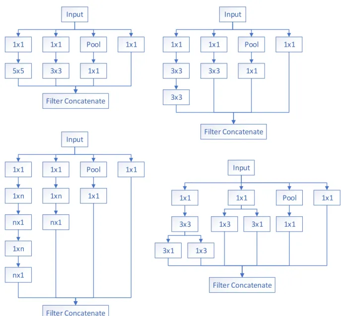
Inception V3 went a step further and reduced the larger 5x5 kernel convolutions to two 3x3 kernel convolutions in series. This saved significant processing resources and still allowed the network to capture some of the advanced dependencies that a 5x5 convolution would capture. The new modifications also established a methodol-ogy to reduce grid size, while expanding the filter banks. This allows for additional complexity while reducing computation time. Further developments reducing convo-lution computations in the inception layers included those which alternated between 1xnlayers andnx1. [67] selectedn= 7 for these layers, and in later layers the second 3x3 convolutions were replaced with parallel 1x3 and 3x1 kernel convolution layers, as seen in Figure 5. Inception V3 utilized batch normalization as a regularizer for con-volution layers, and had a customized regularization scheme through label smoothing on the classifier level.

2.7.4 ResNet

ResNet, presented in [37], addressed the issues of vanishing gradients. In deep CNNs the weight updates can be disproportionately updated in the latter layers, leaving the early layers untrained. Deeper networks begin to degrade as the depth increase which causes accuracy to saturate[37]. A sweet spot appears, where the depth and training are both optimized, yet this limits network complexity. The solution presented by [37] includes residual connections as shown in Figure 6.

The hypotheses of [37] is that it is easier to optimize the residual mapping than the original non mapped network. This mapping proved to be successful as the

(43)

perfor-mance of the network derrived from this theory received first place in the ImageNet competition in 2015. Another benefit to this design is that it can still be trained through standard optimization techniques and implemented with standard CNN li-braries without modification. The authors in [37] used Batch Normalization (BN) in between the convolutional layer and the activation, along with the weight initializa-tion techniques described in [21].

2.7.5 InceptionResNet

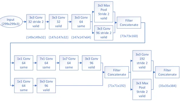
The excellent performance of ResNet and Inception gave the authors in [30] the idea of putting the two technologies together. In many classification networks the earlier layers focus on shrinking the image filter size, and this network begins with the same intent. As seen in Figure 7, the input width and height is halved in the first convolution, but the depth is increased from three colors to 32 filters. To aid the network in retaining information in size reductions, the InceptionResNet v2 utilizes a methodology of concatenating a max pool and convolution, as seen in Figure 7. This was done to aid the network in retaining information that might be useful in classification by including additional convolution and max pooling filters, yet reduce the filter shape to allow quicker processing.

The InceptionResNet pulls a lot of tricks learned from earlier architecture devel-opers. It includes the Inception and ResNet architecture traits discussed earlier, but it also brings aspects used in mobileNet V2, namely linear activation layers as seen in Figure 8. Figure 9 relates the various blocks explained inf Figures 7 and 8. Inception-ResNet V2 utilizes the same padding on each of the block layers, thus allowing the network to be easily adjustable for different image sizes, which allows concatenation and adding residuals without layer scaling. The total filters increases from Blocks

(44)

and the linear activated convolution layer also works as an expansion layer after the concatenation of the earlier layers with 384 filters. This layer runs five times with the addition of residuals for each layer. Blocks B and C work similarly to A with an increase in filters where B runs 128 to 192 filters with a linear expansion layer of 1154, and Block C has 192 to 256 with a linear expansion of 2048 filters.

The authors in [30] found that deep networks can be trained without residual connections, but residual connections improved the training speed greatly. To reduce network over-fitting a 0.2 dropout was used after the global average pooling layer. To allow the network to be trained on a single GPU, batch-normalization was not used on the summation layers. Removing summations’ batch-normalization allowed an increase of inception blocks with the saved processing capabilities. The authors in [30] found that over 1000 filters in residual layers began to develop instabilities in the network, and these results were similar to what was noted in [37]. The authors in [30] developed three networks: InceptionResNet V1, V2, and Inception V4. Inception V4 and InceptionResNet V2 both acheived best-ever performance on the Imagenet classification dataset. Finally an ensemble network (where multiple networks inde-pendently run and results are connected) was performed with one Inception V4 and three InceptionResNet V2 which achieved 3.08% top-5 error.

2.7.6 Xception

The basis of the Xception design is inspired by the Inception architecture[76]. The authors of [76] argues that an Inception module performs similar to a traditional con-volution and depth-wise separable concon-volution hybrid. With the success of depth-wise separable convolution in the mobileNet[28] architectures and the relative lightness compared to traditional convolution, the authors of [76] replaced all convolution layers with depth-wise separable convolutions. As seen in Figure 10, the Xception network

(45)

appears to more closely resemble the ResNet[37] network than the Inception[67], but because of the depth-wise separable layers the actual functionality is more of a hybrid between the two. Xception is much smaller than the behemoth InceptionResNet[30] and is approximately the size of Inception V3[67] and ResNet50[37]. Benchmark per-formance on the ImageNet dataset Xception achieved a .945 accuracy compared to .941, and .933 to Inception V3 and ResNet-152 respectively[76]. While the Xception advancement seems only incremental, it does portray the understanding that different linear modules with residuals can operate similar to directed acyclic ones.

2.7.7 DenseNet

What if every convolutional layer in your network had access to the outputs from every previous layer? The authors in [31] decided to do just that. Since the network did not need to relearn redundant feature maps, the authors in [31] argues that the network requires fewer parameters than traditional convolutional networks. A primary difference from DenseNet architecture and ResNet[37], is DenseNet utilizes a concatenation of the previous input with the output of the current layer as opposed to adding the various layers. DenseNet utilizes what the authors in [31] calls a composite function containing batch normalization and ReLU after a 3×3 convolution layer. The output of the composite function is concatenated with the input then passed to the next composite function as seen in Figure 11. The composite function begins with a bottleneck 1×1 convolution layer with 128 filters. This is done to reduce the input feature-maps and make the larger convolution more efficient[31]. This is again followed by a batch normalization and a ReLU activation with the 3×3 convolution layer containing only 32 filters. because of the filter concatenation across the network as seen in Figure 11, each composite function needs to only perform a small piece[31]. The Network performs a specific amount of composite functions in a dense block

(46)

then uses a transition layer to compress the network. This compression begins with a 1×1 convolution to reduce the filter dimensionality, then a 2×2 average pool with a stride of two to halve the output size. The performance of DenseNet on the ImageNet dataset was competitive with the other leading networks with a top-5 accuracy of .947 with a multi-crop testing and .939 without[31]. The DenseNet architecture provides an effective way to make each layer in a CNN more efficient and applicable to later convolutional layers and the dense classification layer.

(47)

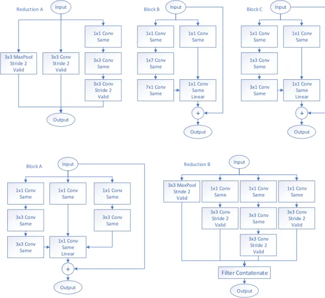
Input 1x1 1x1 Pool 1x1 5x5 3x3 1x1 Filter Concatenate Input 1x1 1x1 Pool 1x1 3x3 3x3 1x1 Filter Concatenate 3x3 Input 1x1 1x1 Pool 1x1 1xn 1xn 1x1 Filter Concatenate nx1 1xn nx1 nx1 Input 1x1 1x1 Pool 1x1 3x3 1x1 Filter Concatenate 3x1 1x3 1x3 3x1

Figure 5. Inception Modules. Top left is the original Inception module. Top right has the 5x5 convolution replaced with two 3x3 convolutions. Bottom left is a middle layer where n= 7, used to reduce computational complexity. Bottom right is a lower layer used to reduce computations of 3x3 convolution.

(48)

Weight Layer Weight Layer

+

Input Output ReLU ReLU

Figure 6. An example of a residual connection. Earlier layers are added to the results of latter layers. Filter Concatenate Input (299x299x3) (149x149x32) 3x3 Conv 32 stride 2 valid 3x3 Conv 32 valid (147x147x32) 3x3 Conv 64 same (147x147x64) 3x3 Max Pool Stride 2 valid 3x3 Conv 96 stride 2 valid (73x73x160) 1x1 Conv 64 same 1x1 Conv 64 same 3x3 Conv 96 valid 7x1 Conv 64 same 1x7 Conv 64 same 3x3 Conv 96 valid (71x71x192) 3x3 Max _Pool Stride 2 valid 3x3 Conv 192 stride 2 valid (35x35x384) Filter Concatenate Filter Concatenate

Figure 7. The introduction layers to the Inception ResNet v2. Each convolutional and pooling layer states the kernel size on the top row, the filters and stride on the second, and the padding, either same padding (which retains original shape), or valid padding, which reduces it according to the convolution/pooling output. The text underneath each box is the output size based with relation to the input.

(49)

3x3 MaxPool Stride 2 Valid + Input Output Block A 3x3 Conv Stride 2 Valid 3x3 Conv Same 1x1 Conv Same 3x3 Conv Stride 2 Valid 3x3 Conv Same Input Output 1x1 Conv Same 3x3 Conv Same 1x1 Conv Same 1x1 Conv Same Linear Reduction A Block B Reduction B Block C 1x1 Conv Same 3x3 Conv Same + 7x1 Conv Same Input Output 1x7 Conv Same 1x1 Conv Same 1x1 Conv Same 1x1 Conv Same Linear Input Output 3x3 Conv Stride 2 Valid 1x1 Conv Same 1x1 Conv Same 3x3 Conv Stride 2 Valid 3x3 MaxPool Stride 2 Valid 1x1 Conv Same 3x3 Conv Same 3x3 Conv Stride 2 Valid Filter Contatenate + 3x1 Conv Same Input Output 1x3 Conv Same 1x1 Conv Same 1x1 Conv Same 1x1 Conv Same Linear

Figure 8. Modules used in InceptionResNet V2. Reduction A and B are used after blocks A and B respectively, and are used to reduce network dimensionality. Each block is tailored for its location in the network.

Input Stem 5x Block A Reduction A 10x Block B Reduction B 5x Block C Average

Pooling Dropout (0.2) Output

Figure 9. Architecture diagram for Inception-ResNet V2. Blocks based on figure 8 and figure 7

(50)

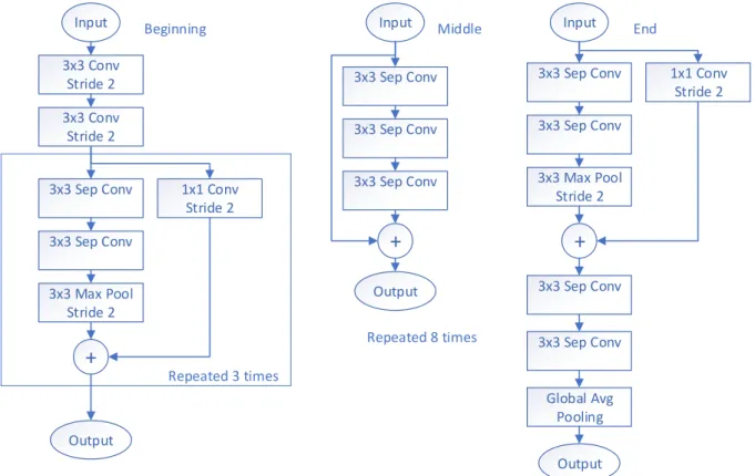
Input Output Beginning Middle

+

Input Output Input Output 3x3 Conv Stride 2 3x3 Conv Stride 2 3x3 Sep Conv 3x3 Sep Conv 3x3 Max Pool Stride 2 1x1 Conv Stride 2

+

Repeated 3 times 3x3 Sep Conv 3x3 Sep Conv 3x3 Sep Conv Repeated 8 times End 3x3 Sep Conv 3x3 Sep Conv 3x3 Max Pool Stride 2 1x1 Conv Stride 2

+

3x3 Sep Conv 3x3 Sep Conv Global Avg Pooling

Figure 10. An overview of the Xception architecture. The begining section reduces dimensionality, the middle increases abstraction, and the end prepares the output.

1x1 3x3 Filter Contatenate 1x1 3x3 Filter Contatenate 1x1 3x3 Filter Contatenate 1x1 3x3 1x1 3x3 1x1 3x3 Input Input Output Output

Figure 11. An example of a three composite function dense block from DenseNet. Top is the implementation, and the bottom displays the composite function’s connectivity.

(51)

III. Methodology

This chapter discusses the techniques and methods used for the experiments in this study. It is composed of five sections: Dataset 3.1, System Architecture 3.2, Hyper-parameter Comparison 3.3, Convolutional Neural Network (CNN) Model Architecture Comparison 3.4, and Custom Loss Development 1.2. The dataset section covers the in-depth origin and formatting of the satellite images to represent an appropriate aerial dataset. Section 3.1 also discusses dataset formatting techniques for the various convolutional neural networks (CNNs). System Architecture details the programming structures, the machine learning architectures, and CNN designs specific to this thesis. The Hyper-parameter Comparison provides the procedure for comparing nine hyper-parameters. CNN Model Architecture Comparison in section 3.4 describes the process for comparing seven innovative CNN models. Finally, Custom Loss Development, section 1.2, discusses a loss specifically designed to integrate the results of a network into an algorithm with Inertial Measurement Unit (IMU) data to provide a more accurate location.

3.1 Dataset

The dataset for this project is built from satellite imagery from multiple seasons and viewing angles. The dataset covers the Dayton, OH area, and is composed of 676 very high resolution satellite images for the training set and 112 for the test set. The images are processed into smaller sizes designed to represent aerial photographs and to be small enough to process adequately in a deep CNN. Each sample image is created using satellite imagery by modeling the view as seen from an aircraft at a specific altitude and orientation. The location coordinates for the center-point of each sample image are localized in a navigation North East Down (NED) coordinate system.

(52)

Altitude ranges are based off the image size and area. The following subsections describe the process that was created to take large, raw satellite images and create small sample images that appear similar to how an aircraft would view the scene.

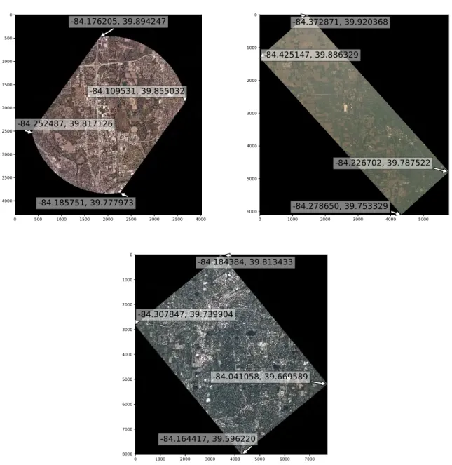
3.1.1 Satellite Images 0 500 1000 1500 2000 2500 3000 3500 4000 0 500 1000 1500 2000 2500 3000 3500 4000 -84.252487, 39.817126 -84.176205, 39.894247 -84.185751, 39.777973 -84.109531, 39.855032 0 1000 2000 3000 4000 5000 0 1000 2000 3000 4000 5000 6000 -84.425147, 39.886329 -84.372871, 39.920368 -84.278650, 39.753329 -84.226702, 39.787522 0 1000 2000 3000 4000 5000 6000 7000 0 1000 2000 3000 4000 5000 6000 7000 8000 -84.307847, 39.739904 -84.184384, 39.813433 -84.164417, 39.596220 -84.041058, 39.669589

Figure 12. Imagery from the training dataset. Each selected image is from a different satellite. Image 1 is the smallest image in the training dataset and was taken April 2016, image 2 was taken July 2016. Image 3 is the largest image in the dataset and was taken October 2016. The coordinates of the corners are indicated in WGS84.

(53)

The dataset used for this project contains spatially-organized raw satellite images that cover 57 total square miles of the area surrounding Dayton, Ohio; 8.08 miles east to west and 7.04 miles north to south. The data was received through a partnership with Air Force Research Laboratory (AFRL), and is sourced from satellite images through AFRL’s relationship with Planet Labs Inc. The average raw image size is 139 million pixels, with the largest at 185 million and the smallest at 39 million pixels. The raw images are original footage from various satellites managed by Planet Labs Inc. over the focus area. A sample of the raw images is displayed in Figure 12. Each image has the WGS84 coordinates of its corners stored in a corresponding .json file. Most of Planet Labs Inc’s satellites have a low earth, polar or nearly polar, sun synchronous orbit[39] which means that the satellite always has sunlight. On the other hand this causes a major shortcoming, a lack of night images. Since test flights designed to accompany this dataset were intended for day time, the data shortcomings were accepted, but additional work is needed for real world viability. Due to the nearly polar orbits, the satellite images have a rotation with respect to North, as seen in Figure 12.

3.1.2 Location Formatting

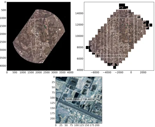
The area of interest has a boundary that is a nearly square polygon of Dayton, Ohio. The first step in the processing chain to create sample images is to pass each satellite’s boundary coordinates through a geometry based identifier to determine if any portion of the raw image’s footprint is within the Dayton bounding box. Only satellite images that contain areas inside the Dayton bounding box are included in the dataset for further processing.

A local navigation coordinate system is established based on the Dayton bounding box boundaries. The center of the bounding box is used for the reference point for the