A combined SMOTE and PSO based RBF classifier for two-class imbalanced problems

(1)

A combined SMOTE and PSO based RBF classiﬁer for two-class

imbalanced problems

Ming Gao

a

, Xia Hong

a,

, Sheng Chen

b

, Chris J. Harris

b a

School of Systems Engineering, University of Reading, Reading RG6 6AY, UK

b_{School of Electronics and Computer Science, University of Southampton, Southampton SO17 1BJ, UK}

a r t i c l e

i n f o

Article history: Received 7 March 2011 Received in revised form 26 May 2011

Accepted 5 June 2011 Communicated by K. Li Available online 28 June 2011 Keywords:

Imbalanced classiﬁcation Synthetic minority over-sampling technique

Radial basis function classiﬁer Orthogonal forward selection Particle swarm optimisation

a b s t r a c t

This contribution proposes a powerful technique for two-class imbalanced classification problems by combining the synthetic minority over-sampling technique (SMOTE) and the particle swarm optimisa-tion (PSO) aided radial basis funcoptimisa-tion (RBF) classifier. In order to enhance the significance of the small and specific region belonging to the positive class in the decision region, the SMOTE is applied to generate synthetic instances for the positive class to balance the training data set. Based on the over-sampled training data, the RBF classifier is constructed by applying the orthogonal forward selection procedure, in which the classifier’s structure and the parameters of RBF kernels are determined using a PSO algorithm based on the criterion of minimising the leave-one-out misclassification rate. The experimental results obtained on a simulated imbalanced data set and three real imbalanced data sets are presented to demonstrate the effectiveness of our proposed algorithm.

1. Introduction

A classiﬁcation problem is referred to as imbalanced when the instances in one or several classes, known as the majority classes, outnumber the instances of the other classes, called the minority classes. Such an imbalance in the data represents the so-called between-class imbalance [1], in contrast to the related issue of within-class imbalance [2,3]. Imbalanced problems widely exist in the ﬁelds of medical diagnosis, science and engineering, and some examples includes surveillance of nosocomial infection[4], cardiac care[5]and elucidating protein–protein interactions[6] as well as fraud detection[7,8], network intrusion detection[9] and telecommunication management [10]. Note that, in an imbalance problem, the minority classes are usually the more important classes. For instance, 11% of patients suffer from one or more nosocomial infections[4]. In the study of two-class imbal-anced problems, the instances in the majority class are referred to as negative, while in its counterpart, the minority class, the instances are referred to as positive. Since in practice the minority class is more important, one should be more concerned with the positive instances. Imbalanced data learning has been widely

researched [11–16]. Typically, the approaches for solving the imbalanced problem can be divided into two categories: re-sampling methods and imbalanced learning algorithms.

The re-sampling approach is actually a re-balancing process to balance the given imbalanced data set. The studies[17,18] on class distribution have shown that balanced data sets provide better classification performance than imbalanced ones, though some other studies [1,19] have argued that imbalanced data sets are not necessarily responsible for the poor performance of some classifiers. Re-sampling techniques are attractive under most imbal-anced circumstances. This is because re-sampling adjusts only the original training data set, instead of modifying the learning algo-rithm. Thus, this approach is external and transportable[18,20], and it provides a convenient and effective way to deal with imbal-anced learning problems using standard classifiers. Specifically, the re-sampling methods include the random over-sampling, which randomly appends replicated instances to the positive class, and the random under-sampling, which randomly removes instances from the majority class. Alternatively, there exist the guided over-sampling and under-over-sampling, respectively, of which the choices to replicate or to eliminate are informed rather than random. In addition, the synthetic minority over-sampling technique (SMOTE) [21]is a well acknowledged over-sampling method. In the SMOTE, instead of mere data oriented duplicating, the positive class is over-sampled by creating synthetic instances in the feature space formed by the positive instances and theirK-nearest neighbours.

Contents lists available atScienceDirect

journal homepage:www.elsevier.com/locate/neucom

Neurocomputing

Corresponding author.

E-mail addresses:[email protected] (M. Gao), [email protected] (X. Hong), [email protected] (S. Chen), [email protected] (C.J. Harris).

(2)

The second category, consisting of imbalanced learning algo-rithms, can be regarded as a process to modify or re-balance the existing learning algorithms so that they can deal with imbal-anced problems effectively. The imbalimbal-anced learning algorithms include the cost-sensitive method [22–25], the discrimination-based and recognition-discrimination-based approaches[3]. An alternative is to adapt standard kernel-based or radial basis function (RBF) classi-ﬁers, which use a ﬁxed common variance for every RBF kernel and choose RBF centres from input data, to imbalanced data sets by modifying the kernel construction and model selection procedure. A representative work[26]of this imbalanced learning proposes a regularised weighted least square estimator (LSE) using the orthogonal forward selection (OFS) based on the model selection criterion of maximising the leave-one-out (LOO) area under the curve (AUC) of receiver operating characteristics (ROC). In this LOO-AUCþOFS algorithm [26], the cost function of the LSE is made sensitive to the class labels, such that the errors due to minority class data samples are given a higher weight

r

Z1, and

this weighted LSE (WLSE) reduces to the standard LSE with the weight

r

¼1. A well-known RBF modelling is the two staged procedure [27], in which the RBF centres are ﬁrst determined using the

k

-means clustering[28]and the RBF weights are then obtained using the LSE. To cope with imbalanced data sets, a natural extension of[27]is to modify the latter stage as the WLSE, where the same weighted cost function of [26] is used. This

k

-means þWLSE algorithm provides a viable alternative within this imbalanced learning category.

Kernel-based learning, such as support vector machine (SVM) and RBF, is widely used for solving balanced learning problems. In particular, a powerful approach for constructing the RBF and other sparse kernel classifiers is to assign a fixed common variance for every kernel and to select input data as the candidate centres for RBF kernels by minimising the leave-one-out (LOO) misclassification rate in the efficient OFS procedure [29]. This approach has its root in regression application [30–33]. Two limitations may be associated with this ‘‘fixed’’ RBF kernel approach. Firstly, RBF kernels cannot be flexibly tuned, as the position of each kernel is restricted to the input data and the shape of each kernel is fixed rather than determined by the learning procedure. Secondly, the common kernel variance has to be determined via cross validation, which inevitably increases the computational cost. The previous studies[34–36] have proposed to construct the tunable RBF classifier based on the OFS procedure using a global search optimisation algorithm[37]to optimise the RBF kernels one by one. This tunable RBF kernel approach is observed to produce sparser classifiers with better performance but higher computational complexity in classifier construction, in comparison with the standard fixed kernel approach. Recently, the particle swarm optimisation (PSO) algorithm[38]is adopted to minimise the LOO misclassification rate in the OFS construction of tunable RBF classifier[39,40]. PSO[38]is an efficient popula-tion-based stochastic optimisation technique inspired by social behaviour of bird flocks or fish schools, and it has been success-fully applied to wide-ranging optimisation applications[41–46]. Owing to the efficiency of PSO, the tunable RBF modelling approach advocated in [39,40] offers significant advantages in terms of better generalisation performance and smaller classifier size as well as lower complexity in learning process, compared with the standard fixed kernel approach. This PSO aided tunable RBF classifier offers the state-of-the-art for balanced data sets.

Although the study[1]has shown that kernel-based methods provide a relatively robust classification to imbalanced problems, the detrimental effects of a highly imbalanced data set can seriously degrade the generalisation performance of kernel-based classifiers. In order to achieve better classification performance for highly imbalanced data, an effective approach is to integrate

kernel-based classifiers with re-sampling methods. The previous studies[47–49] mainly focused on SVMs. Specifically, the method [47]combined the SMOTE with different costs to bias SVMs by assigning different classes with different costs so as to shift the decision boundary away from the positive instances and to define a better boundary. The work[48]proposed ensemble systems by re-sampling data sets to form the input to the standard SVM classifier, while the method[49]introduced asymmetric misclas-sification costs in SVMs so as to improve clasmisclas-sification perfor-mance. Another integration of SVM with under-sampling method used the combination of the granular support vector machine (GSVM) [50] and repetitive under-sampling (RU) to form the GSVM–RU algorithm[51].

Against this background, this contribution proposes an effec-tive alternaeffec-tive to deal with two-class imbalanced classification problems by combining the SMOTE algorithm [21]and the PSO aided RBF classifier[39,40]. Specifically, the SMOTE is first applied to generate synthetic instances in the positive class to balance the training data set. Using the resulting balanced data set, the tunable RBF classifier is then constructed by applying the PSO to minimise the LOO misclassification rate in the computationally efficient OFS procedure. In the experimental study involving a simulated imbalanced data set and three real imbalanced data sets, three benchmarks are used to compare with the proposed SMOTEþPSO-OFS method. The first benchmark combines the SMOTE[21]and theK nearest neighbourðK-NNÞclassifier[52], which will be denoted as the SMOTEþK-NN. TheK-NN classifier is a widely used classification method, and this combined SMOTE and K-NN represents a typical method of the re-sampling approach for imbalanced problems. The second benchmark is the algorithm advocated in[26], denoted by the LOO-AUCþOFS, which is a state-of-the-art representative of the second approach for dealing with imbalanced problems. The third benchmark, the

k

-meansþWLSE algorithm, as discussed previously, is also a typical method of the imbalanced learning approach. The experi-mental results obtained demonstrate that the proposed method is competitive to these existing state-of-the-arts methods for two-class imbalanced problems.

The rest of the paper is organised as follows. Section 2 introduces the tunable RBF model for two-class classification and the OFS procedure based on the LOO misclassification rate, while Section 3 presents the PSO algorithm for tuning the RBF kernels by minimising the LOO misclassification rate. Section 4 introduces the SMOTE method and presents the proposed com-bined SMOTE and PSO based RBF algorithm. The effectiveness of our approach is demonstrated by numerical examples in Section 5, and our conclusions are given in Section 6.

2. RBF classiﬁer for two-class problems

Consider the two-class data setDN¼ fxk,ykgNk¼1that containsN

data instances, where yk¼ f71gdenotes the class label for the

feature vectorxkARm, while there areN_þ positive instances and Nnegative instances, withN¼NþþN. We use the data setDN

to construct the RBF classiﬁer of the form: ^ yðMÞk ¼ XM i¼1 wigiðxkÞ ¼gTMðkÞwM ~ yðMÞ_k ¼sgnðy^ðMÞ_k Þ ð1Þ

whereMis the number of RBF kernels,y^ðMÞ_k is the output of the M-term classiﬁer with the M kernels,giðÞ for 1rirM, wM¼

½w1w2 wMT is the weight vector and gTMðkÞ ¼ ½g1ðxkÞ

(3)

class label forxk, and

sgnðyÞ ¼ 1, yr0 1, y40

(

ð2Þ In this study, we use the Gaussian kernel function

giðxÞ ¼expððxciÞT

R

1i ðxciÞÞ ð3Þ

where ciARm is the centre vector of the ith RBF kernel and

Ri

¼diagf

s

2

i,1,

s

2 i,2, ,

s

2

i,mgis the diagonal covariance matrix of the ith kernel. Hence, the position of each kernel,ci, and the coverage

of each kernel,

Ri

, are both considered as the tunable parameters to be determined in modelling.

From (1), the RBF classiﬁer over DN can be written in the

matrix form as y¼GMwMþeðMÞ _ð4Þ whereeðMÞ_{¼ ½}_eðMÞ 1 e ðMÞ 2 e ðMÞ N T

is the error vector with theM-term modelling error eðMÞ_k ¼yky^

ðMÞ

k , y¼ ½y1y2 yNT is the desired

class label vector, and the kernel matrixGM¼ ½g1g2 gM with

gl¼ ½glðx1Þglðx2Þ glðxNÞT for 1rlrM. Note that gl is the lth

column ofGMwhilegT

MðkÞis thekth row ofGM.

Now consider the orthogonal decomposition GM¼PMAM, where AM¼ 1 a1,2 a1,M 0 1 & ^ ^ _{& &} _a_M1_,_M 0 0 1 2 6 6 6 4 3 7 7 7 5 ð5Þ PM¼ ½p1p2 pM ð6Þ

and the columns in (6) satisfypT

ipj¼0 foriaj. The RBF classiﬁer

(4) can alternatively be represented as

y¼PMhMþeðMÞ _ð7Þ

where

hM

¼ ½y1

y

2

y

MTsatisﬁes

hM

¼AMwM. The space spanned

by the original model bases gi, 1rirM, is identical to that

spanned bypi, 1rirM.

The OFS procedure constructs the RBF kernels one by one by minimising the LOO misclassiﬁcation rate[39,40]. Speciﬁcally, at thenth stage, the nth RBF kernel, namely, pn and

y

n, is

deter-mined. Deﬁne the LOO-model output of the n-term RBF model constructed from the LOO data setDN\ðxk,ykÞ, calculated atxk, as

^

yðn_k,kÞ. Further deﬁne the associated LOO decision variable as sðn_k,kÞ¼sgnðykÞy^

ðn,kÞ k ¼yky^

ðn,kÞ

k ð8Þ

Then the LOO misclassiﬁcation rate is deﬁned by[29] JðnÞ_LOO¼1

N XN k¼1

Idðsðnk,kÞÞ ð9Þ

in which the indicator functionIdðsÞis deﬁned as

IdðsÞ ¼

1, sr0 0, s40

(

ð10Þ The LOO misclassification rate is a measure of the classifier’s generalisation capability [29,35,36,53]. By making use of Sherman–Morrison–Woodbury theorem[53]as well as the ortho-gonal property, the LOO decision variable can be efficiently calculated according to[29,39,40] sðn_k,kÞ¼

c

ðnÞ k

Z

ðnÞ k ð11Þ

in which

c

ðnÞ_k and

Z

ðnÞk can be computed recursively by

c

ðnÞ_k ¼

c

ðn1Þ_k þyk

y

npnðkÞ p 2 nðkÞ pT npnþl ð12Þ

Z

ðnÞ k ¼

Z

ðn1Þ k p2 nðkÞ pT npnþl ð13Þ where pn(k) is the kth element of pn, and

l

Z0 is a small

regularisation parameter if the regularisation is employed. At the nth stage of the OFS procedure, the nth RBF kernel, namely, its centre vectorcn and diagonal covariance matrix

Rn

, are determined by minimisingJ_LOOðnÞ . The construction terminates at the size ofMwhenJ_LOOðMþ1ÞZJðMÞ

LOO[29,39,40].

3. PSO for optimising RBF parameters

Denote

l

¼ ½

m

ð1Þ

m

ð2Þ

m

ð2mÞT as the 2m-dimensional para-meter vector that contains cn and

Rn

. Then, as deﬁned in the previous section, the problem of determining thenth RBF kernel’s parameters at the nth OFS stage is to solve the following optimisation problem ^

l

¼arg min lACJ ðnÞ LOOð

l

Þ ð14Þ

where the 2m-dimensional search space

C

is deﬁned by

C

9Y 2m

i¼1

½Gi,min,

G

i,max ð15Þ

Speciﬁcally, the search space forcn¼ ½cn,1cn,2 cn,mTis speciﬁed

by the distribution of the training datafxk¼ ½xk,1xk,2 xk,mTgNk¼1,

namely,

cn,iA½x_min_,_i,x_max_,_i9½G_i_,_min,

G

_i_,_max ð16Þ

for 1rirm, with xmin,i¼ min 1rkrNxk,i xmax,i¼ max 1rkrNxk,i 8 < : ð17Þ

while each element of

Rn

is limited in the range

s

2

n,iA½

s

2_min,

s

2_max9½G_ði_þmÞ_,_min,

G

_ði_þmÞ_,_max ð18Þ

for 1rirm. When applying a PSO[38]to solve the optimisation (14), a swarm of the candidate particlesf

l

½l

i g S

i¼1 are ‘‘ﬂying’’ in

the search space

C

in order to ﬁnd a solution

l

^, whereSis the size of the swarm andlAf0,1, ,Lgdenotes thelth movement of the swarm. Each particle

l

has a 2m-dimensional velocity

m

¼ ½

n

ð1Þ

n

ð2Þ

n

ð2mÞT to direct its search, and

m

AV with the

velocity space deﬁned by

V9Y 2m

i¼1

½Vi,max,Vi,max ð19Þ

whereVi,max¼12ðGi,maxGi,minÞ.

To start the PSO, the candidate particlesf

l

½0_i gS_i_¼₁are initialised randomly within

C

, and the velocity for each candidate particle is initialised to zero, namely,f

m

½0i ¼0g

S

i¼1. The cognitive information pb½l_i and the social information gb½l record the best position visited by the particleiand the best position visited by the entire swarm, respectively, during the l movements. The LOO costs associated with pb½li and gb

½l

are denoted by JLOOðnÞ ðpb ½l iÞ and

J_LOOðnÞ ðgb½lÞ, respectively. The cognitive information pb½l_i and the

(4)

positions according to

m

½lþ1 i ¼a

m

½l i þrandðÞ b ðpb ½l i

l

½l iÞ þrandðÞ c ðgb ½l

l

½l i Þ ð20Þ

l

½liþ1¼

l

½l i þ

m

½lþ1 i ð21Þ

whereadenotes the inertia weight,randðÞis the random number uniformly distributed in [0, 1],bandcare the two acceleration coefﬁcients. Experimental results given in[40]show that a better performance can be achieved by using a¼randðÞ instead of a constant inertia weight. Adopting the time varying acceleration coefﬁcients (TVAC)[41], in which

b¼2:5ð2:50:5Þ l=L

c¼0:5þ ð2:50:5Þ l=L ð22Þ

can often enhance the performance of PSO. The search space

C

and the velocity space V are used to conﬁne

l

½lþ1 i and

m

½lþ1 i

derived from (20) and (21), respectively. If

m

½lþ1

i becomes too

close to0, a random re-initialisation is needed, which may take the form

m

½liþ1¼70:1randðÞ Vmax, where Vmax¼ ½V1,maxV2,max

V2m,maxT. The detailed PSO aided OFS algorithm can be found

in[40], also see the next section.

4. Combined SMOTE and PSO optimised RBF for imbalanced classiﬁcation

The SMOTE [21]over-samples the positive class by creating synthetic instances by a speciﬁed over-sampling ratio of the original minority data size,

b

%. Based on each minority data sample, denoted byxo,

b

%synthetic data points are generated by randomly selecting data points on the lines linkingxowith some of itsKnearest neighbours, whereKis predetermined. Depending on the required SMOTE amount

b

%, one out of the K nearest positive-class data samples are randomly selected several times. For example, if

b

%¼600%andK¼5, then one out of ﬁve nearest neighbours of xo is randomly chosen repeatedly for six times. Each time a random kth neighbour is selected to create a line linkingxoto this neighbour, and then a single synthetic instance is created by randomly selecting a point on the line. Thus any synthetic instancexsis given by

xs¼xoþd ðxftg

o xoÞ ð23Þ

where xsdenotes one synthetic instance,xftgo is thetth nearest

neighbors of xo in the positive class, and

d

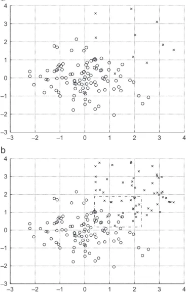
A½0,1 is a random

number. The procedure is repeated for all the positive data points. A major problem caused by imbalanced data sets is that most classifiers tend to attribute the positive-class instances within the decision region to the negative class, due to insuffi-cient positive-class training instances in the decision region. As a result, the trained decision boundary tends to be far away from the negative class and too close to the positive class. The contribution of SMOTE is to enhance the significance of the small and specific region belonging to the positive class in the decision region, which leads to the better generalisation for classifiers. Fig. 1(a) shows a simulated imbalanced data set, the details of which are specified in Section 5. After the SMOTE over-sampling the positive class by 500% of its original size, the instances from the positive class become more significant in the decision region (the area specified by dash–dot line), as shown inFig. 1(b), compared with the original data set. Consequently, the trained decision boundary tends to be further away from the posi-tive class.

We combine this SMOTE with the PSO optimised RBF classiﬁer described in Section 3 to create a powerful algorithm for two-class imbalanced problems. This combined SMOTE and PSO aided RBF is detailed below.

1. Over-sampling the training data set:

(a) SMOTE initialisation: Specify the balanced degree

b

%and the value ofK.

(b) Create the new training data set D~N by appending the

generated positive training data points to the original training data set via the SMOTE.

2. PSO aided OFS initialisation:

(a) Specify the search space

C

and the velocity space V. Specify the values ofLandS.

(b) SetJ_LOOð0Þ ¼1,

c

ð0Þ_k ¼0, and

Z

ð0Þk ¼1.

(c) Set regularisation parameter

l

¼106_.

3. Construct thenth RBF kernel:

(a) PSO initialisation: Randomly initialisef

l

½0i g S i¼1in

C

, and setf

m

½0i ¼0g S i¼1. (b) For 0rloL: –3 –2 –1 0 1 2 3 4 –3 –2 –1 0 1 2 3 4 –3 –2 –1 0 1 2 3 4 –3 –2 –1 0 1 2 3 4

Fig. 1.Simulated 2-dimensional example: (a) original training data space, and (b) training data space after SMOTE over-sampling the positive class by 500% of its original size, where x denotes a positive-class instance whileJdenotes a negative class instance.

(5)

(b.i) Construct the candidatesgfign from

l

½li , for 1rirS. Then,

for 1rirSand 1rjon, compute:

afig j,n¼ 1, n¼1 pT jg fig n pT jpj , n41 8 > > < > > : pfig n ¼ gfign, n¼1 gfign X n1 j¼1 afig_j_,_npj, n41 8 > > < > > :

y

fig_n ¼ ðp fig nÞTy ðpfignÞTpfign þl

(b.ii) For 1rirSand 1rkrN, compute:

c

ðnÞ_k fig ¼

c

ðn1Þ_k þyðkÞyfignpfignðkÞ

ðpfignðkÞÞ2 ðpfig nÞTpfign þl

Z

ðnÞk fig ¼

Z

ðn1Þ k ðpfignðkÞÞ2 ðpfignÞTpfign þl

Then, for 1rirS, calculate the LOO costs: J_LOOðnÞ fig ¼1 N XN k¼1 Id

c

ðnÞ_k fig

Z

ðnÞ k fig ! (b.iii) For 1rirS: IfJðnÞ_LOOfigoJ_LOOðnÞ ðpb½l_iÞ: pb½l_i ¼

l

½l i andJ ðnÞ LOOðpb ½l i Þ ¼J ðnÞ LOOfig Then ﬁnd in¼arg min 1rirSJ ðnÞ LOOðpb ½l i Þ IfJðnÞ_LOOðpb½l_i nÞoJ ðnÞ LOOðgb ½l Þ: gb½l¼pb½l_i n andJ ðnÞ LOOðgb ½l Þ ¼JðnÞ_LOOðpb½l_i nÞ (b.iv) For 1rirS:

m

½lþ1 i ¼a

m

½l i þrandðÞ b ðpb ½l i

l

½l iÞ þrandðÞ c ðgb½l

l

½li Þ If

n

½lþ1 i ðjÞ ¼0:

n

½liþ1ðjÞ ¼70:1randðÞ Vj,max If

n

½lþ1 i ðjÞ4Vj,max:

n

½liþ1ðjÞ ¼Vj,max If

n

½lþ1 i ðjÞoVj,max:

n

½lþ1i ðjÞ ¼ Vj,max Then for 1rirS:

l

½liþ1¼

l

½l i þ

m

½lþ1 i If

m

½lþ1 i ðjÞ4

G

j,max:

m

½liþ1ðjÞ ¼

G

j,max If

m

½lþ1 i ðjÞo

G

j,min:

m

½liþ1ðjÞ ¼

G

j,min

(c) Termination of PSO: gb½L providescn and

Rn

with the associated LOO costJLOOðnÞ ¼J

ðnÞ LOOðgb

½L

Þ.

The algorithm also generatesaj,nfor 1rjon,pnand

y

n

as well as

c

ðnÞ_k and

Z

ðnÞk for 1rkrN.

4. OFS termination condition checking:

IfJðnÞ_LOOoJðn1Þ_LOO :n¼nþ1, go to step 3.

Otherwise,M¼n1, terminate the OFS procedure.

5. Experimental results

The effectiveness of the proposed SMOTEþPSO-OFS algorithm was investigated using a simulated imbalanced date set and three real imbalanced data sets. The ﬁrst two real data sets were taken from[54], while the third real data set was from[55]. These three real data sets were chosen in the order of increasing imbalance. For each data set, the positive class was over-sampled at different rates

b

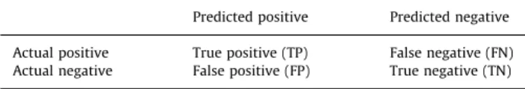
% of its original size using the SMOTE. For the synthetic data set, a separate test data set was used, while for the three real data sets,P-fold cross validation was used, to indicate the classifier generalisation capability based on multiple specifica-tions, including the true positive rate (TP%) and the false positive rate (FP%) [56], as well as the precision (Pr), the F-measure (F-meas) and the G-mean [57]. These criteria are commonly adopted as the performance metrics for evaluating imbalanced learning classifiers. They were calculated according to the confu-sion matrix inTable 1as follows:

TP%¼ TP TPþFN ð24Þ FP%¼ FP FPþTN ð25Þ Pr¼ TP TPþFP ð26Þ G-mean¼pffiffiffiffiffiffiffiffiffiffiffiffiffiffiffiffiffiffiffiffiffiffiffiffiffiffiffiffiffiffiffiffiffiffiffiTP% ð1FP%Þ ð27Þ F-meas¼2PrTP% PrþTP% ð28Þ

As discussed in the introduction section, the three typical methods that represent the two different approaches for dealing with imbalanced problems, respectively, were used as the bench-marks for comparison, and they were the SMOTEþK-NN with K¼1 and 3, as well as the LOO-AUCþOFS with different weight

r

and the

k

-meansþWLSE with different weight

r

. Note that in the SMOTEþK-NN classiﬁers if there is any data sample in the test data set that duplicates a data sample in the training data set, this was not counted in the statistics in order to obtain honest cross validation. This is necessary in particular for ADI data sets which are produced by randomly sampling the original data set, causing repetitive data samples. For the

k

-means þWLSE algorithm a ﬁxed common variance for every kernel was predetermined empirically (similar to [26]), and in addition the number of centres were also predetermined empirically.

Simulated imbalanced data set: The simulated data set was generated with the m¼2 features. The mean vector of the negative class was [0 0]T_{, while the mean vector of the positive} class was [2 2]T_{. The covariance matrices of both the} negative-class and positive-negative-class instances were the same 2-dimensional identity matrix. The training data set contained 100 instances from the negative class and 10 instances from the positive class, as depicted inFig. 1(a). The test data set contained 1000 instances from the negative class, and 100 instances from the positive class. The 5-nearest neighbour method was applied to generate syn-thetic training data in the SMOTE, with the over-sampling rate

b

% set to 0%, 100%, 500%, 1000%, 1500% and 2000%, respectively. For the SMOTEþPSO-OFS, the swarm size and the number of Table 1

Confusion matrix.

Predicted positive Predicted negative Actual positive True positive (TP) False negative (FN) Actual negative False positive (FP) True negative (TN)

(6)

movements were set toS¼10 andL¼20. The test results obtained by the various classiﬁers are shown inTable 2.

It can be seen from the results for the SMOTEþPSO-OFS listed inTable 2that, as the over-sampling rate

b

%increases, typically TP% increases but FP% inevitably increases as well. A better tradeoff between TP% and FP% was achieved, however, at the over-sampling rate where the betterG-mean andF-measure were obtained. Since the imbalance degree of the negative class to the positive class was 10:1, the over-sampled positive instances made_D~_N _{fully balanced at}

_b

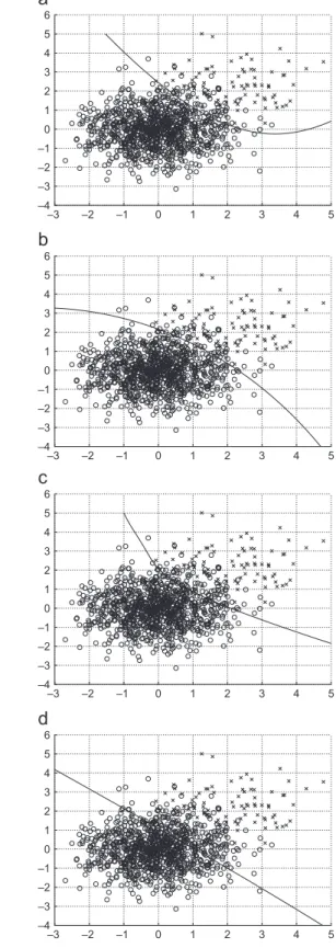
_%_¼₁₀₀₀_%_{. From}_{Table 2, it can be} seen that the best test performance tradeoff occurred at the over-sampling rate around 500–1000%. Compared with the other

benchmark methods, the proposed SMOTEþPSO-OFS showed a competitive test performance. The effect of the SMOTE on the decision boundary is shown in Fig. 2, where it can be seen that the decision boundary trained by the more balanced data set was pushed further away from the positive class.

–3 –2 –1 0 1 2 3 4 5 –4 –3 –2 –1 0 1 2 3 4 5 6 –3 –2 –1 0 1 2 3 4 5 –4 –3 –2 –1 0 1 2 3 4 5 6 –3 –2 –1 0 1 2 3 4 5 –4 –3 –2 –1 0 1 2 3 4 5 6 –3 –2 –1 0 1 2 3 4 5 –4 –3 –2 –1 0 1 2 3 4 5 6

Fig. 2.Decision boundaries obtained by the SMOTEþPSO-OFS with different over-sampling rates for the simulated 2-dimensional example: (a) b%¼0%, (b)

b%¼100%, (c)b%¼1000%, and (d)b%¼2000%, where x denotes a positive-class test instance whileJdenotes a negative-class test instance.

Table 2

Test classiﬁcation performance comparison for the synthetic data set.

Method TP% FP% Pr G-mean F-meas

SMOTEþ1-NN 0.830 0.047 0.638 0.899 0.722 ðb%¼0%Þ SMOTEþ1-NN 0.880 0.094 0.484 0.893 0.624 ðb%¼100%Þ SMOTEþ1-NN 0.920 0.113 0.449 0.903 0.603 ðb%¼500%Þ SMOTEþ1-NN 0.930 0.156 0.373 0.886 0.533 ðb%¼1000%Þ SMOTEþ1-NN 0.940 0.158 0.373 0.890 0.534 ðb%¼1500%Þ SMOTEþ1-NN 0.930 0.150 0.383 0.889 0.542 ðb%¼2000%Þ SMOTEþ3-NN 0.780 0.022 0.780 0.873 0.780 ðb%¼0%Þ SMOTEþ3-NN 0.900 0.092 0.495 0.904 0.638 ðb%¼100%Þ SMOTEþ3-NN 0.940 0.134 0.412 0.902 0.573 ðb%¼500%Þ SMOTEþ3-NN 0.950 0.156 0.378 0.895 0.541 ðb%¼1000%Þ SMOTEþ3-NN 0.950 0.151 0.386 0.898 0.549 ðb%¼1500%Þ SMOTEþ3-NN 0.950 0.174 0.353 0.886 0.515 ðb%¼2000%Þ LOO-AUCþOFS 0.860 0.049 0.637 0.904 0.732 ðr¼1Þ LOO-AUCþOFS 0.840 0.028 0.750 0.903 0.792 ðr¼5Þ LOO-AUCþOFS 0.900 0.063 0.588 0.918 0.712 ðr¼10Þ LOO-AUCþOFS 0.870 0.046 0.654 0.911 0.747 ðr¼15Þ LOO-AUCþOFS 0.870 0.049 0.640 0.909 0.737 ðr¼20Þ k-meansþWLSE 0.810 0.030 0.730 0.886 0.768 ðr¼1Þ k-meansþWLSE 0.840 0.041 0.672 0.898 0.747 ðr¼5Þ k-meansþWLSE 0.860 0.078 0.524 0.890 0.652 ðr¼10Þ k-meansþWLSE 0.940 0.131 0.418 0.904 0.578 ðr¼15Þ k-meansþWLSE 0.950 0.185 0.339 0.880 0.500 ðr¼20Þ SMOTEþPSO-OFS 0.860 0.044 0.662 0.907 0.748 ðb%¼0%Þ SMOTEþPSO-OFS 0.880 0.055 0.615 0.912 0.724 ðb%¼100%Þ SMOTEþPSO-OFS 0.810 0.023 0.780 0.890 0.794 ðb%¼500%Þ SMOTEþPSO-OFS 0.890 0.053 0.627 0.918 0.736 ðb%¼1000%Þ SMOTEþPSO-OFS 0.930 0.102 0.476 0.914 0.631 ðb%¼1500%Þ SMOTEþPSO-OFS 0.940 0.110 0.461 0.915 0.618 ðb%¼2000%Þ

(7)

Pima Indians diabetes data set: The data set was obtained from the UCI repository[54], and it contained 768 instances from the two classes with 500 negative instances and 268 positive instances. This data set was used to identify the positive diabetes cases in a population near Phoenix, Arizona. The feature space dimension wasm¼8. All the eight input features were normalised

to the range [0, 1] using the operation xk,i¼

xk,ixmin,i xmax,ixmin,i

, 1rkrN, 1rirm ð29Þ The 5-nearest neighbour scheme was applied to generate syn-thetic training data in the SMOTE. The over-sampling rate

b

%was

Table 3

Eight-fold cross validation classiﬁcation performance and standard deviations for Pima Indians diabetes data set.

SMOTEþ1-NN 0.5470.04 0.2170.04 0.5870.06 0.6570.02 0.5670.04 ðb%¼0%Þ SMOTEþ1-NN 0.5870.06 0.2470.04 0.5670.07 0.6670.03 0.5770.05 ðb%¼50%Þ SMOTEþ1-NN 0.5970.06 0.2570.04 0.5670.07 0.6670.02 0.5770.06 ðb%¼75%Þ SMOTEþ1-NN 0.6370.06 0.2770.05 0.5570.08 0.6770.02 0.5870.05 ðb%¼100%Þ SMOTEþ1-NN 0.6670.05 0.2770.05 0.5770.07 0.7070.03 0.6170.05 ðb%¼150%Þ SMOTEþ1-NN 0.6870.07 0.2870.04 0.5670.07 0.7070.04 0.6170.06 ðb%¼200%Þ SMOTEþ1-NN 0.7070.04 0.3070.04 0.5570.07 0.7070.03 0.6170.04 ðb%¼250%Þ SMOTEþ1-NN 0.7270.04 0.3670.07 0.5270.09 0.6870.04 0.6070.05 ðb%¼500%Þ SMOTEþ3-NN 0.5870.06 0.1770.06 0.6570.07 0.6970.04 0.6170.04 ðb%¼0%Þ SMOTEþ3-NN 0.6270.07 0.1970.05 0.6370.05 0.7070.04 0.6270.04 ðb%¼50%Þ SMOTEþ3-NN 0.6770.07 0.2570.05 0.5970.06 0.7170.04 0.6370.06 ðb%¼75%Þ SMOTEþ3-NN 0.7070.08 0.2970.05 0.5670.05 0.7170.05 0.6270.04 ðb%¼100%Þ SMOTEþ3-NN 0.7470.08 0.3070.04 0.5670.05 0.7270.04 0.6470.04 ðb%¼150%Þ SMOTEþ3-NN 0.7670.09 0.3370.06 0.5570.06 0.7170.05 0.6470.06 ðb%¼200%Þ SMOTEþ3-NN 0.7870.07 0.3470.05 0.5570.07 0.7270.03 0.6470.06 ðb%¼250%Þ SMOTEþ3-NN 0.8270.06 0.4170.05 0.5270.07 0.7070.03 0.6370.06 ðb%¼500%Þ LOO-AUCþOFS 0.5870.03 0.1370.05 0.7070.09 0.7170.03 0.6370.05 ðr¼1:0Þ LOO-AUCþOFS 0.6870.06 0.2070.07 0.6570.08 0.7370.04 0.6670.05 ðr¼1:5Þ LOO-AUCþOFS 0.7370.05 0.2470.07 0.6270.07 0.7470.04 0.6770.05 ðr¼2:0Þ LOO-AUCþOFS 0.7770.05 0.3170.06 0.5770.05 0.7370.03 0.6670.07 ðr¼2:5Þ k-meansþWLSE 0.6070.06 0.1370.05 0.7270.07 0.7270.04 0.6570.03 ðr¼1:0Þ k-meansþWLSE 0.7070.08 0.2070.07 0.6570.07 0.7470.06 0.6770.05 ðr¼1:5Þ k-meansþWLSE 0.7770.07 0.2970.07 0.5970.07 0.7470.06 0.6670.06 ðr¼2:0Þ k-meansþWLSE 0.8470.05 0.3470.07 0.5770.06 0.7570.06 0.6870.06 ðr¼2:5Þ SMOTEþPSO-OFS 0.5770.04 0.1170.04 0.7370.10 0.7170.03 0.6470.06 ðb%¼0%Þ SMOTEþPSO-OFS 0.7070:07 0.1970.09 0.6770.07 0.7570.03 0.6870.04 ðb%¼50%Þ SMOTEþPSO-OFS 0.7370.12 0.2370.19 0.6870.14 0.7370.06 0.6970.04 ðb%¼75%Þ SMOTEþPSO-OFS 0.7970.07 0.2570.10 0.6470.06 0.7670.05 0.7070.04 ðb%¼100%Þ SMOTEþPSO-OFS 0.8170.07 0.2970.09 0.6070.06 0.7670.04 0.6970.05 ðb%¼150%Þ SMOTEþPSO-OFS 0.8370.04 0.3370.07 0.5870.06 0.7570.04 0.6870.05 ðb%¼200%Þ SMOTEþPSO-OFS 0.8570.07 0.3570.07 0.5770.07 0.7470.06 0.6870.06 ðb%¼250%Þ SMOTEþPSO-OFS 0.9170.05 0.4470.06 0.5270.05 0.7170.04 0.6770.05 ðb%¼500%Þ

(8)

set to 0%, 50%, 75%, 100%, 150%, 200%, 250% and 500%, respec-tively. The swarm size and the number of movements were set to

S¼10 andL¼20 for the PSO. The 8-fold cross validation was used

to investigate the test performance of a classiﬁer. The 8-fold cross validation results for the various classiﬁers are shown inTable 3. For the SMOTEþPSO-OFS, it can be seen that the best TP%, that is, the best detection capability for diabetes, occurred at

b

%¼500%, while the best FP% occurred at

b

%¼0%. But the best TP% was obtained at the expense of the worst FP%, and the best FP% was obtained at the expense of the worst TP%, as indicated by the poor values of theG-mean andF-measure. The best tradeoff between TP% and FP% occurred around

b

%¼1002150%, which enabled to detect as many positive diabetes patients as possible while ensuring the minimum incorrect diagnose of healthy people. As expected, this best over-sampling rate made the enlarged data set fully balanced. The results ofTable 3also show that the test performance of the proposed SMOTEþPSO-OFS compare favourably with the other classiﬁers.

Haberman survival data set: This data set in the UCI repository [54] contained 306 instances from the two classes with 225 negative instances and 81 positive instances. It came from a study on the survival of patients after surgery for breast cancer.

The feature space dimension was m¼3. All the three input features were normalised to the range [0, 1] using the operation (29). The 5-nearest neighbour method was adopted to generate synthetic training data in the SMOTE. The over-sampling rate

b

% was set to 0%, 100%, 200%, 300% and 400%, respectively. The swarm size and the number of movements were chosen to be

S¼10 andL¼20. The 3-fold cross validation was used to calculate

test performance, and the results obtained for the various classi-ﬁers are shown inTable 4. Compared with the other benchmark classiﬁers, the SMOTEþPSO-OFS demonstrated its competitive performance. For the SMOTEþPSO-OFS, the best tradeoff between TP% and FP% occurred around

b

%¼150%, which was again close to the imbalanced degree of the original data set.

ADI data set: The austempered ductile iron (ADI) material data set was obtained from a study on fatigue cracks from the graphite nodules within the microstructure in an automotive camshaft application [55]. This two-class data set contained 2923 instances in the feature space of dimension m¼9, with 2807 negative instances and 116 positive instances. As in[55,26], 700 negative-class instances and 90 positive-class instances were randomly selected from the original data set to form the 8-fold cross validation set. Initially, all the nine input features were Table 4

Three-fold cross validation classiﬁcation performance and standard deviations for Haberman survival data set.

SMOTEþ1-NN 0.2870.06 0.2070.13 0.3870.12 0.4770.02 0.3170.02 ðb%¼0%Þ SMOTEþ1-NN 0.3670.11 0.2270.16 0.4170.12 0.5270.03 0.3670.01 ðb%¼100%Þ SMOTEþ1-NN 0.4170.13 0.2870.14 0.3670.05 0.5370.04 0.3770.04 ðb%¼200%Þ SMOTEþ1-NN 0.4470.29 0.2770.21 0.4070.09 0.5370.08 0.3870.09 ðb%¼300%Þ SMOTEþ1-NN 0.4770.20 0.2970.22 0.4070.11 0.5570.02 0.4070.04 ðb%¼400%Þ SMOTEþ3-NN 0.3070.10 0.1570.10 0.4570.14 0.4970.08 0.3570.09 ðb%¼0%Þ SMOTEþ3-NN 0.4170.07 0.2170.14 0.4570.13 0.5670.04 0.4170.06 ðb%¼100%Þ SMOTEþ3-NN 0.4970.15 0.2470.18 0.4670.10 0.6070.03 0.4570.04 ðb%¼200%Þ SMOTEþ3-NN 0.5370.19 0.2870.20 0.4470.09 0.6070.04 0.4670.05 ðb%¼300%Þ SMOTEþ3-NN 0.5670.16 0.3170.21 0.4370.09 0.6070.02 0.4670.01 ðb%¼400%Þ LOO-AUCþOFS 0.2170.02 0.0570.01 0.6170.05 0.4570.02 0.3170.03 ðr¼1Þ LOO-AUCþOFS 0.3870.08 0.1370.02 0.5170.02 0.5770.05 0.4470.06 ðr¼2Þ LOO-AUCþOFS 0.6270.08 0.2770.03 0.4570.05 0.6770.05 0.5270.06 ðr¼3Þ LOO-AUCþOFS 0.6770.02 0.4270.08 0.3670.03 0.6270.03 0.4770.02 ðr¼4Þ k-meansþWLSE 0.2070.02 0.0270.00 0.6370.05 0.4470.02 0.3070.03 ðr¼1Þ k-meansþWLSE 0.3670.06 0.0570.01 0.4670.03 0.5870.04 0.4070.04 ðr¼2Þ k-meansþWLSE 0.4970.03 0.1070.01 0.3970.02 0.6770.02 0.4470.01 ðr¼3Þ k-meansþWLSE 0.5670.04 0.1470.01 0.3470.01 0.6970.02 0.4270.01 ðr¼4Þ SMOTEþPSO-OFS 0.2370.04 0.0770.06 0.5770.01 0.4470.05 0.3170.05 ðb%¼0%Þ SMOTEþPSO-OFS 0.4470.09 0.1570.06 0.5270.09 0.6170.07 0.4870.09 ðb%¼100%Þ SMOTEþPSO-OFS 0.6370.06 0.2370.06 0.5070.07 0.6970.08 0.5570.09 ðb%¼200%Þ SMOTEþPSO-OFS 0.8070.09 0.5870.07 0.3470.05 0.5770.09 0.4770.05 ðb%¼300%Þ SMOTEþPSO-OFS 0.8470.08 0.6970.08 0.3170.04 0.5170.08 0.4570.05 ðb%¼400%Þ

(9)

normalised to within the range [0, 1] using the operation (29). The SMOTE adopted the 5-nearest neighbour scheme to generate synthetic training data. The over-sampling rate

b

%was set to 0%, 100%, 300%, 500%, 800%, 1000%, 1500% and 2000%, respectively.

The swarm size and the number of movements were set toS¼10

andL¼20 for the PSO. The 8-fold cross validation results obtained

by the various classiﬁers are shown in Table 5. For the SMO-TEþPSO-OFS, the best overall test performance was achieved at Table 5

Eight-fold cross validation classiﬁcation performance and standard deviations for ADI data set.

SMOTEþ1-NN 0.3270.07 0.0870.01 0.1370.03 0.5470.06 0.1970.04 ðb%¼0%Þ SMOTEþ1-NN 0.4470.10 0.1270.02 0.1170.03 0.6270.07 0.1870.04 ðb%¼100%Þ SMOTEþ1-NN 0.5170.13 0.1970.02 0.0970.02 0.6470.09 0.1570.04 ðb%¼300%Þ SMOTEþ1-NN 0.5870.14 0.2270.02 0.0970.02 0.6770.08 0.1570.04 ðb%¼500%Þ SMOTEþ1-NN 0.6270.12 0.2670.02 0.0870.02 0.6770.07 0.1470.03 ðb%¼800%Þ SMOTEþ1-NN 0.6670.13 0.2770.02 0.0870.02 0.6970.07 0.1470.03 ðb%¼1000%Þ SMOTEþ1-NN 0.6970.14 0.3170.02 0.0770.02 0.6970.07 0.1370.03 ðb%¼1500%Þ SMOTEþ1-NN 0.7370.14 0.3470.02 0.0770.01 0.6970.07 0.1370.02 ðb%¼2000%Þ SMOTEþ3-NN 0.2370.08 0.0470.01 0.1870.06 0.4670.08 0.2070.07 ðb%¼0%Þ SMOTEþ3-NN 0.3970.14 0.1170.01 0.1270.03 0.5970.10 0.1870.06 ðb%¼100%Þ SMOTEþ3-NN 0.5770.02 0.1770.01 0.1170.03 0.6870.10 0.1870.05 ðb%¼300%Þ SMOTEþ3-NN 0.6570.15 0.2270.02 0.1070.03 0.7170.08 0.1770.04 ðb%¼500%Þ SMOTEþ3-NN 0.6970.16 0.2870.02 0.0870.02 0.7070.09 0.1570.04 ðb%¼800%Þ SMOTEþ3-NN 0.7370.17 0.3070.02 0.0870.02 0.7170.09 0.1570.03 ðb%¼1000%Þ SMOTEþ3-NN 0.7670.16 0.3470.02 0.0770.01 0.7070.08 0.1470.03 ðb%¼1500%Þ SMOTEþ3-NN 0.7770.13 0.3870.03 0.0770.01 0.6970.06 0.1370.02 ðb%¼2000%Þ LOO-AUCþOFS 0.2170.03 0.0170.01 0.6770.08 0.4670.03 0.3270.04 ðr¼1Þ LOO-AUCþOFS 0.5570.09 0.1470.02 0.3370.02 0.6870.05 0.4170.04 ðr¼5Þ LOO-AUCþOFS 0.7170.05 0.2270.03 0.3070.01 0.7470.02 0.4270.01 ðr¼10Þ LOO-AUCþOFS 0.7770.02 0.2570.02 0.2870.01 0.7670.01 0.4170.02 ðr¼15Þ LOO-AUCþOFS 0.8870.03 0.3670.04 0.2470.02 0.7570.02 0.3770.02 ðr¼20Þ k-meansþWLSE 0.1970.03 0.0270.00 0.6170.05 0.4370.03 0.2970.03 ðr¼1Þ k-meansþWLSE 0.6270.03 0.1770.02 0.3270.02 0.7270.01 0.4270.02 ðr¼5Þ k-meansþWLSE 0.8070.03 0.2770.02 0.2870.02 0.7770.02 0.4270.02 ðr¼10Þ k-meansþWLSE 0.8770.02 0.3470.03 0.2570.02 0.7570.02 0.3870.02 ðr¼15Þ k-meansþWLSE 0.9170.02 0.4470.03 0.2170.01 0.7170.02 0.3470.02 ðr¼20Þ SMOTEþPSO-OFS 0.2070.04 0.0170.01 0.7070.09 0.4470.04 0.3070.03 ðb%¼0%Þ SMOTEþPSO-OFS 0.3070.07 0.0470.02 0.5370.09 0.5570.05 0.3970.03 ðb%¼100%Þ SMOTEþPSO-OFS 0.5170.07 0.1170.03 0.3870.04 0.6770.02 0.4370.02 ðb%¼300%Þ SMOTEþPSO-OFS 0.7270.09 0.2370.06 0.2970.03 0.7470.02 0.4170.03 ðb%¼500%Þ SMOTEþPSO-OFS 0.7770.07 0.2870.08 0.2770.03 0.7470.02 0.4070.03 ðb%¼800%Þ SMOTEþPSO-OFS 0.8270.04 0.2970.04 0.2770.02 0.7670.01 0.4170.01 ðb%¼1000%Þ SMOTEþPSO-OFS 0.8970.04 0.3570.04 0.2570.02 0.7670.02 0.3970.02 ðb%¼1500%Þ SMOTEþPSO-OFS 0.8870.02 0.3570.03 0.2470.02 0.7570.02 0.3870.02 ðb%¼2000%Þ

(10)

the over-sampling rate around

b

%¼1000% to 1500%, and the SMOTEþPSO-OFS showed a competitive performance to the other methods.

6. Conclusions

The RBF classifier performs well on balanced or slightly imbalanced data sets, and our previous work has provided an efficient and tunable RBF classifier optimised by the PSO based on the OFS procedure. For highly imbalanced data sets, however, the performance of the tunable RBF classifier may no longer be satisfactory. In order to combat challenging imbalanced classifi-cation problems, many approaches have been proposed, which aim to reduce the influence from the underlying imbalanced distribution. In particular, the SMOTE is effective to increase the significance of the positive class in the decision region. In this contribution, we have proposed a powerful and efficient algo-rithm for solving two-class imbalanced problems, referred to as the SMOTEþPSO-RBF, by combining the SMOTE and the PSO optimised RBF classifier. The experimental results presented in this study have demonstrated that the proposed SMOTEþPSO-RBF offers a very competitive solution to other existing state-of-the-arts methods for combating imbalanced classification problems.

Acknowledgements

This work was supported by UK EPSRC. The authors would like to thank Dr. P.A.S. Reed and Dr. K.K. Lee for their help with ADI data set.

References

[1] N. Japkowicz, S. Stephen, The class imbalance problem: a systematic study, Intell. Data Anal. 6 (5) (2002) 429–449.

[2] G.M. Weiss, Mining with rarity: a unifying framework, ACM SIGKDD Explor. Newsl. 6 (1) (2004) 7–19.

[3] N. Japkowicz, Concept-learning in the presence of between-class and within-class imbalances, in: E. Stroulia, S. Matwin (Eds.), Advances in Artiﬁcial Intelligence, vol. 2056, Springer-Verlag, Berlin, 2001, pp. 67–77.

[4] G. Cohen, M. Hilario, H. Sax, S. Hugonnet, A. Geissbuhler, Learning from imbalanced data in surveillance of nosocomial infection, Artif. Intell. Med. 37 (2006) 7–18.

[5] R.B. Rao, S. Krishnan, R.S. Niculescu, Data mining for improved cardiac care, ACM SIGKDD Explor. Newsl. 8 (1) (2006) 3–10.

[6] C. Yu, L. Chou, D. Chang, Predicting protein–protein interactions in unba-lanced data using the primary structure of proteins, BMC Bioinformatics 11 (1) (2010) 167–177.

[7] F. Provost, T. Fawcett, R. Kohavi, The case against accuracy estimation for comparing induction algorithms, in: Proceedings of the 15th International Conference on Machine Learning, Madison, USA, July 24–27, 1998, pp. 445–453.

[8] T. Fawcett, F. Provost, Adaptive fraud detection, Data Min. Knowl. Discovery 1 (1997) 291–316.

[9] D.A. Cieslak, N.V. Chawla, A. Striegel, Combating imbalance in network intrusion datasets, in: Proceedings of the 2006 IEEE International Conference on Granular Computing, Atlanta, USA, May 10–12, 2006, pp. 732–737. [10] G.M. Weiss, H. Hirsh, Learning to predict rare events in event sequences, in:

Proceedings of the Fourth IEEE International Conference on Knowledge Discovery and Data Mining, New York, USA, August 27–31, 1998, pp. 359–363.

[11] F. Provost, Machine Learning from Imbalanced Data Sets 101, AAAI Workshop on Learning from Imbalanced Data Sets, 2000.

[12] H. He, A. Garcia, Learning from imbalanced data, IEEE Trans. Knowl. Data Eng. 21 (9) (2009) 1263–1284.

[13] R. Barandela, J.S. Sa´nchez, V. Garcı´a, E. Rangel, Strategies for learning in class imbalance problems, Pattern Recognition 36 (2003) 849–851.

[14] V. Garcıá, J.S. Sańchez, R.A. Mollineda, R. Alejo, J.M. Sotoca, The Class Imbalance Problem in Pattern Classification and Learning, in: II Congreso Espan˜ ol de Informa´tica, 2007, pp. 283–291.

[15] N.V. Chawla, D.A. Cieslak, L.O. Hall, A. Joshi, Automatically countering imbalance and its empirical relationship to cost, Data Min. Knowl. Discovery 17 (2) (2008) 225–252.

[16] G.M. Weiss, K. McCarthy, B. Zabar, Cost-sensitive learning vs. sampling: which is best for handling unbalanced classes with unequal error costs?, in: Proceedings of the 2007 IEEE International Conference on Data Mining, 2007, pp. 35–41. [17] G.M. Weiss, F. Provost, Learning when training data are costly: the effect of

class distribution on tree induction, Artif. Intell. Res. 19 (2003) 315–354. [18] A. Estabrooks, T. Jo, N. Japkowicz, A multiple resampling method for learning

from imbalanced data sets, J. Chem. Inf. Modeling 20 (1) (2004) 18–36. [19] G.E.A.P.A. Batista, R.C. Prati, M.C. Monard, A study of the behavior of several

methods for balancing machine learning training data, SIGKDD Explor. Newsl. 6 (1) (2004) 20–29.

[20] C. Drummond, R.C. Holte, C4.5, class imbalance, and cost sensitivity: Why under-sampling beats over-sampling, in: 2003 International Conference on Machine Learning—Workshop Learning from Imbalanced Datasets II, Washington DC, USA, August 21, 2003, pp. 1–8.

[21] N.V. Chawla, K.W. Bowyer, L.O. Hall, Smote: synthetic minority over-sam-pling technique, J. Artif. Intell. Res. 16 (2002) 321–357.

[22] C. Elkan, The foundations of cost-sensitive learning, in: Proceedings of the 17th International Joint Conference on Artiﬁcial Intelligence, Seattle, USA, August 4–10, 2001, pp. 973–978.

[23] K.M. Ting, An instance-weighting method to induce cost-sensitive trees, IEEE Trans. Knowl. Data Eng. 14 (3) (2002) 659–665.

[24] M.A. Maloof, Learning when data sets are imbalanced and when costs are unequal and unknown, in: 2003 International Conference on Machine Learning—Workshop Learning from Imbalanced Datasets II, Washington DC, USA, August 21, 2003, pp. 1–8.

[25] K. McCarthy, B. Zabar, G. Weiss, Does cost-sensitive learning beat sampling for classifying rare classes? in: Proceedings of the First International Work-shop on Utility-Based Data Mining, Chicago, USA, August 21, 2005, pp. 69–77. [26] X. Hong, S. Chen, C.J. Harris, A kernel-based two-class classiﬁer for

imbal-anced data sets, IEEE Trans. Neural Networks 18 (1) (2007) 28–41. [27] J. Moody, C.J. Darken, Fast learning in networks of locally-tuned processing

units, Neural Comput. 1 (1989) 281–294.

[28] S. Haykin, Neural Networks: A Comprehensive Foundation, second ed., Prentice Hall, Upper Saddle River, NJ, 1999.

[29] X. Hong, S. Chen, C.J. Harris, A fast linear-in-the-parameters classiﬁer construction algorithm using orthogonal forward selection to minimize leave-one-out misclassiﬁcation rate, Int. J. Syst. Sci. 39 (2) (2008) 119–125. [30] S. Chen, C.F.N. Cowan, P.M. Grant, Orthogonal least squares learning

algo-rithm for radial basis function networks, IEEE Trans. Neural Networks 2 (2) (1991) 302–309.

[31] X. Hong, P.M. Sharkey, K. Warwick, Automatic nonlinear predictive model construction using forward regression and the press statistic, IEE Proc. Control Theory Appl. 150 (3) (2003) 245–254.

[32] X. Hong, P.M. Sharkey, K. Warwick, A robust nonlinear identiﬁcation algo-rithm using press statistic and forward regression, IEEE Trans. Neural Net-works 14 (2) (2003) 454–458.

[33] S. Chen, X. Hong, C.J. Harris, P.M. Sharkey, Sparse modelling using orthogonal forward regression with PRESS statistic and regularization, IEEE Trans. Syst. Man Cybern. 34 (2) (2004) 898–911.

[34] S. Chen, X.X. Wang, X. Hong, C.J. Harris, Kernel classiﬁer construction using orthogonal forward selection and boosting with Fisher ratio class separability measure, IEEE Trans. Neural Networks 17 (6) (2006) 1652–1656.

[35] S. Chen, X. Hong, C.J. Harris, Construction of RBF classiﬁers with tunable units using orthogonal forward selection based on leave-one-out misclassiﬁcation rate, in: Proceedings of the 2006 International Joint Conference on Neural Networks, Vancouver, Canada, July 16–21, 2006, pp. 6390–6394.

[36] S. Chen, X. Hong, B.L. Luk, C.J. Harris, Construction of tunable radial basis function networks using orthogonal forward selection, IEEE Trans. Syst. Man, Cybern. Part B 39 (2) (2009) 457–466.

[37] S. Chen, X.X. Wang, C.J. Harris, Experiments with repeating weighted boosting search for optimization in signal processing applications, IEEE Trans. Syst. Man Cybern. Part B 35 (4) (2005) 682–693.

[38] J. Kennedy, R.C. Eberhart, Swarm Intelligence, Morgan Kaufmann, 2001. [39] S. Chen, X. Hong, C.J. Harris, Radial basis function classiﬁer construction using

particle swarm optimisation aided orthogonal forward regression, in: Pro-ceedings of the 2010 International Joint Conference on Neural Networks, Barcelona, Spain, July 18–23, 2010, pp. 3418–3423.

[40] S. Chen, X. Hong, C.J. Harris, Particle swarm optimization aided orthogonal forward regression for uniﬁed data modelling, IEEE Trans. Evol. Comput. 14 (4) (2010) 477–499.

[41] A. Ratnaweera, S.K. Halgamuge, Self-organizing hierarchical particle swarm optimizer with time-varying acceleration coefﬁcients, IEEE Trans. Evol. Comput. 8 (3) (2004) 240–255.

[42] W.-F. Leong, G.G. Yen, PSO-based multiobjective optimization with dynamic population size and adaptive local archives, IEEE Trans. Syst. Man Cybern. Part B 38 (5) (2008) 1270–1293.

[43] S. Chen, X. Hong, B.L. Luk, C.J. Harris, Non-linear system identiﬁcation using particle swarm optimisation tuned radial basis function models, Int. J. Bio-Inspired Comput. 1 (4) (2009) 246–258.

[44] M. Ramezani, M.-R. Haghifam, C. Singh, H. Seiﬁ, M.P. Moghaddam, Determi-nation of capacity beneﬁt margin in multiarea power systems using particle swarm optimization, IEEE Trans. Power Syst. 24 (2) (2009) 631–641. [45] S. Chen, W. Yao, H.R. Palally, L. Hanzo, Particle swarm optimisation aided

MIMO transceiver designs, in: Y. Tenne, C.-K. Goh (Eds.), Computational Intelligence in Expensive Optimization Problems, Springer-Verlag, Berlin, 2010, pp. 487–511.

(11)

[46] H.L. Wei, S.A. Billings, Y. Zhao, L.Z. Gu, Lattice dynamical wavelet neural networks implemented using particle swarm optimization for spatio-tem-poral system identiﬁcation, IEEE Trans. Neural Networks 20 (1) (2009) 181–185.

[47] R. Akbani, S. Kwek, N. Japkowicz, Applying support vector machines to imbalanced datasets, in: Proceedings of the 15th European Conference on Machine Learning, Pisa, Italy, September 20–24, 2004, pp. 39–50. [48] P. Kang, S. Cho, Eus svms: ensemble of under-sampled svms for data

imbalance problems, in: Proceedings of the 13th International Conference on Neural Information Processing, Hong Kong, China, October 3–6, 2006, pp. 837–846.

[49] B.X. Wang, N. Japkowicz, Boosting support vector machines for imbalanced data sets, in: Proceedings of the 17th International Conference on Founda-tions of Intelligent Systems, Toronto, Canada, May 20–23, 2008, pp. 38–47. [50] Y. Tang, Y.-Q. Zhang, Z. Huang, X. Hu, Granular svm-rfe gene selection

algorithm for reliable prostate cancer classiﬁcation on microarray expression data, in: Proceedings of the 5th IEEE Symposium on Bioinformatics and Bioengineering, Minneapolis, USA, October 19–21, 2005, pp. 290–293. [51] Y. Tang, Y.-Q. Zhang, Granular svm with repetitive undersampling for highly

imbalanced protein homology prediction, in: Proceedings of the 2006 IEEE International Conference on Granular Computing, Atlanta, USA, May 10–12, 2006, pp. 457–460.

[52] T. Cover, P. Hart, Nearest neighbor pattern classiﬁcation, IEEE Trans. Inf. Theory 13 (1) (1967) 21–27.

[53] R.H. Myers, Classical and Modern Regression with Applications, second ed., PWS-KENT, Boston, 1990.

[54] C.L. Blake, C.J. Merz, UCI Repository of Machine Learning Databases, Depart-ment of Computer Science, University of California, Irvine, CA, 1998/_http://

archive.ics.uci.edu/ml/datasets.htmlS_.

[55] K.K. Lee, C.J. Harris, S.R. Gunn, P.A.S. Reed, Classiﬁcation of imbalanced data with transparent kernel, in: Proceedings of the 2001 International Joint Conference on Neural Networks, Washington DC, USA, July 15–19, 2001, pp. 2410–2415.

[56] A.P. Bradley, The use of the area under the roc curve in the evaluation of machine learning algorithms, Pattern Recognition 30 (1997) 1145–1159. [57] C. van Rijsbergen, Information Retrieval, Butterworths, London, UK, 1979.

Ming Gaoreceived the MEng degree from Northwes-tern Polytechnical University (NPU), Shaan’xi, P.R. China, in 2006, and the MEng degree from the Beihang University, Beijing, P.R. China, in 2009. He is now working towards the PhD degree in the Systems Engineering School, the University of Reading (UoR), Reading, UK. His research interests are machine learn-ing, pattern recognition, and their applications in imbalanced problems.

Xia Hong received her university education at National University of Defense Technology, P.R. China (BSc, 1984; MSc, 1987), and University of Shefﬁeld, UK (PhD, 1998), all in automatic control. She worked as a Research Assistant in Beijing Institute of Systems Engineering, Beijing, China from 1987 to 1993. She worked as a Research Fellow in the Department of Electronics and Computer Science at University of Southampton from 1997 to 2001. She is currently a Reader at School of Systems Engineering, University of Reading. She is actively engaged in research into non-linear systems identiﬁcation, data modelling, estima-tion and intelligent control, neural networks, pattern recognition, learning theory and their applications. She has published over 100 research papers, and coauthored a research book. She was awarded a Donald Julius Groen Prize by IMechE in 1999.

Sheng Chenreceived his PhD degree in control engi-neering from the City University, London, UK, in September 1986. He was awarded the Doctor of Sciences (DSc) degree by the University of Southamp-ton, SouthampSouthamp-ton, UK, in 2005. From October 1986 to August 1999, he conducted research and academic appointments at the University of Shefﬁeld, the Uni-versity of Edinburgh and the UniUni-versity of Ports-mouth, all in UK. Since September 1999, he has been with the School of Electronics and Computer Science, University of Southampton, UK. Professor Chen’s research interests include wireless communications, adaptive signal processing for communications, machine learning, and evolutionary computation methods. He has published over 400 research papers. Dr. Chen is a Fellow of IET and a Fellow of IEEE. In the database of the world’s most highly cited researchers, compiled by Institute for Scientiﬁc Information (ISI) of the USA, Dr. Chen is on the list of the highly cited researchers (2004) in the engineering category.

Chris Harrisreceived university education at Leicester (BSc), Oxford (MA) and Southampton (PhD). He pre-viously conducted appointments at the Universities of Hull, UMIST, Oxford and Cranﬁeld, as well as being employed by the UK Ministry of Defence. His research interests are in the area of intelligent and adaptive systems theory and its application to intelligent auton-omous systems, management infrastructures, intelli-gent control and estimation of dynamic processes, multi-sensor data fusion and systems integration. He has authored or coauthored 12 books and over 400 research papers, and he was the associate editor of numerous international journals including Automa-tica, Engineering Applications of AI, International Journal of General Systems Engineering, International Journal of System Science and the International Journal on Mathematical Control and Information Theory. He was elected to the Royal Academy of Engineering in 1996, was awarded the IEE Senior Achievement medal in 1998 for his work on autonomous systems, and the highest international award in IEE, the IEE Faraday medal in 2001 for his work in Intelligent Control and Neurofuzzy System.