How To Understand And Understand The Power Of A Powerline Microscope

(1)

DOCSIS

®

Best Practices and Guidelines

Proactive Network Maintenance Using

Pre-equalization

CM-GL-PNMP-V02-110623

RELEASED

Notice

This DOCSIS® guidelines document is the result of a cooperative effort undertaken at the direction of Cable Television Laboratories, Inc. for the benefit of the cable industry and its customers. This document may contain references to other documents not owned or controlled by CableLabs®. Use and understanding of this document may require access to such other documents. Designing, manufacturing, distributing, using, selling, or servicing products, or providing services, based on this document may require intellectual property licenses from third parties for technology referenced in this document.

Neither CableLabs nor any member company is responsible to any party for any liability of any nature whatsoever resulting from or arising out of use or reliance upon this document, or any document referenced herein. This document is furnished on an “AS IS“ basis and neither CableLabs nor its members provides any representation or warranty, express or implied, regarding the accuracy, completeness, noninfringement, or fitness for a particular purpose of this document, or any document referenced herein.

(2)

Document Status Sheet

Document Control Number: CM-GL-PNMP-V02-110623

Document Title: Proactive Network Maintenance Using Pre-equalization Revision History: V01 – Released 4/15/10

V02 – Released 6/23/11 Date: June 23, 2011

Status: Work in Progress

Draft Released Closed

Distribution Restrictions: Author

Only CL/Member CL/ VendorMember/ Public

Key to Document Status Codes

Work in Progress An incomplete document, designed to guide discussion and generate feedback that may include several alternative requirements for consideration.

Draft A document in specification format considered largely complete, but lacking review by Members and vendors. Drafts are susceptible to substantial change during the review process.

Issued A stable document, which has undergone rigorous member and vendor review and is suitable for product design and development, cross-vendor interoperability, and certification testing. Changes to Issued test plans are made through

engineering change (EC) requests.

Closed A static document, reviewed, tested, validated, and closed to further engineering changes to the specification through CableLabs.

Trademarks

CableCARD™, CableHome®, CableLabs®, CableNET®, CableOffice™, CablePC™, DCAS™, DOCSIS®, DPoE™, EBIF™, eDOCSIS™, EuroDOCSIS™, EuroPacketCable™, Go2BroadbandSM, M-Card™, M-CMTS™, OCAP™, OpenCable™, PacketCable™, PCMM™, and tru2way® are marks of Cable Television Laboratories, Inc. All other marks are the property of their respective owners.

(3)

Figures

Figure 1 - Micro-reflection with multiple-transit echoes...13

Figure 2 - Micro-reflection with single impedance mismatch interface...14

Figure 3 - Composite Micro-reflection resulting from Type 1 and Type 2 Micro-reflections ...15

Figure 4 - Upstream Equalizer Structure...16

Figure 5 - CM-CMTS Ranging Interaction Enabling Pre-equalization Process...17

Figure 6 - Range Response Message Format ...18

Figure 7 - Range Request Message Format...19

Figure 8 - CM Pre-eq Coefficients Values and Frequency Response Scenarios...20

Figure 9 - CMTS CM Pre-equalization Coefficients Values and Frequency Response Scenarios ...21

Figure 10 - Pre-equalization Compensation Capabilities under Short and Long Delay Micro-reflection Scenarios ..23

Figure 11 - MIB Format for docsIfCmStatusEqualizationdata ...24

Figure 12 - Proactive Network Maintenance Processes based on Pre-equalization ...25

Figure 13 - Equalizer Structure HEXDECIMAL-to-DECIMAL Conversion...26

Figure 14 - Group Delay increase with increasing cascade depth...31

Figure 15 - Pre Main Tap Energy Increase with Cascade Depth (Fc=40.4 MHz, Ch. W=3.2 MHz, No Micro-reflections, first 12 taps shown )...32

Figure 16 - Pre Main Tap Energy Increase with Cascade Depth (Fc=40.4 MHz, Ch. W=3.2 MHz, with 0.5 μs Micro-reflection, first 12 taps shown ) ...34

Figure 17 - Tap Energy for Different Cascade Depth Scenarios (Fc=14 MHz, Ch. W=3.2 MHz, with 0.5 μs Micro-reflection, first 12 taps shown ) ...35

Figure 18 - Short reference plant block diagram...40

Figure 19 - CM & CMTS Elements Contributing To US Distortion (In Orange)...41

Figure 20 - Pre-equalizer frequency response with (0.5μs, -10 dBc) and without micro-reflection ...43

Figure 21 - Calibrated pre-equalizer frequency response obtained from micro-reflection on (0.5μs, -10 dBc) and off scenarios ...43

Figure 22 - Correlation of Topology with Distortion to Provide Fault Localization...45

Figure 23 - Observation of multiple CMs frequency response...46

Figure 24 - Identified Micro-reflection Patterns...47

Figure 25 - Clustering of Common Micro-reflection Signatures ...47

Figure 26 - Common Micro-reflection Signature - Case A ...48

Figure 27 - Common Micro-reflection Signature - Case B ...49

Figure 28 - Severity Classification Mechanisms ...50

Figure 29 - Micro-reflection amplitude data of same two CMs to highlight trending over time ...51

Figure 30 - CM micro-reflection amplitude over time highlighting intermittent issues...53

Figure 31 - Amplitude vs. Frequency peak/valley of 10.55 dB with echo present in impulse response...57

Figure 32 - Entire upstream scan shows no similar signatures shared by other modems...57

Figure 33 - Distance calculation applied with customer address and mapping...57

Figure 34 - Single customer modem demonstrates the effects of ingress...60

Figure 35 - Multiple modems on the same upstream demonstrate the effects of ingress ...60

Figure 36 - Effects of ingress when mapped ...61

Figure 37 - Time domain representation of typical impulse...69

(6)

Figure 39 - Impulse duration characteristics ...71

Figure 40 - Impulse power level distribution characteristics...71

Figure 41 - Burst/impulse noise lasting N symbol periods requires burst protection of N+1 symbols if the burst crosses symbol boundaries ...72

Figure 42 - Byte Interleaver Operation...73

Figure 43 - Burst robustness (in red) and added latency (in blue) for a 64 byte packet using different FEC and interleaver block size settings...74

Figure 46 - Burst impact on S-CDMA subframe...75

Figure 47 - Burst robustness in microseconds for 16-QAM, 3.2 MHz bandwidth channel with TCM off and diverse FEC and subframe settings (packet occupies at least one subframe) ...76

Figure 48 - Burst robustness in microseconds for 64-QAM, 6.4 MHz bandwidth channel with TCM off and diverse FEC and subframe settings (packet occupies at least one subframe) ...76

Figure I-1 - A filter's time delay-versus-frequency curve often has a bathtub shape ...79

Figure I-2 - Phase-versus-frequency for 100 feet of coax ...81

Figure I-3 - Time delay-versus-frequency for 100 feet of coax ...82

Figure I-4 - Complex frequency response in the return path...83

Figure I-5 - Ideal transmission line model...84

Figure I-6 - Real-world transmission line model...85

Figure I-7 - Creation of reflections in a cable network's feeder plant ...86

Figure I-8 - Graphic representation of incident signal and second reflection ...86

Figure I-9 - Reflection example that will be used to illustrate the formation of amplitude ripple ...87

Figure I-10 - Phasor view of incident signal vector (long arrow) and reflection vector (short arrow) ...88

Figure I-11 - Reflection vector rotated 45 degrees from original position...88

Figure I-18 - Reflection vector back at original position after rotating 360 degrees...90

Figure I-19 - Amplitude-versus-phase plot of phasor view vector sum vectors...90

Figure I-20 - Example of flat amplitude-versus-frequency response ...91

Figure I-21 - Example of tilted or sloped amplitude-versus-frequency response...91

Figure I-22 - Example of upstream 64-QAM signal with substantial in-channel tilt ...91

Figure I-23 - Example of 64-QAM signal after adaptive pre-equalization eliminated most of the in-channel tilt...92

Figure I-24 - A signal carried in the sloped portion of the widely spaced amplitude ripple will exhibit in-channel tilt ...92

Figure I-25 - 64-QAM signal with good (36.3 dB) MER ...92

Figure I-26 - 64-QAM signal with poor (23.2 dB) MER ...93

Figure I-27 - 16-QAM constellation showing target symbol, transmitted (or received ) symbol, and modulation error vectors...94

(7)

Figure I-28 - MER is the ratio of average symbol power to average error power...94

Figure I-29 - QAM receiver block diagram...96

Figure I-30 - Each vector has a real (in-phase or I) and imaginary (quadrature or Q) component ...97

Figure I-31 - Unequalized 64-QAM constellation ...99

Figure I-32 - Equalized 64-QAM constellation...100

Figure I-33 - Generic 4-tap adaptive equalizer...102

Figure I-34 - Amplitude-versus-time plot of an incident signal and micro-reflection...103

Figure I-35 - Amplitude-versus-frequency response...103

Figure I-36 - Phase-versus-frequency response...104

Figure I-37 - Required magnitude- and phase-versus-frequency response to cancel echo...104

Figure I-38 - Adaptive equalizer that will be used in the example in the text...105

Figure I-39 - Operation of the adaptive equalizer's first tap...106

Figure I-40 - Operation of the adaptive equalizer's second tap ...106

Figure I-41 - Summing the outputs of the adaptive equalizer's first and second taps ...107

Figure I-42 - Operation of the adaptive equalizer's third tap...107

Figure I-43 - Summing the output of the adaptive equalizer's third tap with the previously summed first and second taps...108

Figure I-44 - Operation of the adaptive equalizer's fourth tap...108

Figure I-45 - Final summing process provides an equalized output...109

Figure I-46 - Final amplitude and phase-versus-frequency response after adaptive equalization...109

Figure I-47 - Upstream pre-equalization is able to compensate for in-channel tilt ...110

Figure IV-1 - Equivalent Reflection Coefficient ΓE ...115

Figure V-1 - A Multiple Recursion Echo ...117

Figure V-2 - Wring Diagrams To Make Echoes In a Lab ...118

Figure V-3 - A Single Recursion Echo Example...119

Figure V-4 - How A Multiple Recursion Echo Can be Canceled with Pre-distortion ...120

Figure V-5 - Comparison of Signal Path Impulse Responses and Programming for Adaptive Equalizers...121

Figure VI-1 - Software Sequence Diagram SD-PNM200 ...123

(8)

Tables

Table 1 - Maximum Delays Generated by Pre-equalization Filter Structures in DOCSIS 1.1 and 2.0...22

Table 2 - DOCSIS 2.0 and 3.0 Transmit Pre-equalization MIBs ...24

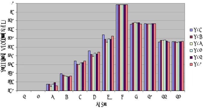
Table 3 - Maximum amplitude and encoding formats for the 16 most popular 2.0 CMs in US ...26

Table 4 - Band-Edge Operation Impact on Tap Energy (no Micro-reflections)...32

Table 5 - Pre-equalization Metrics at Band-Edge (No Micro-reflections) ...33

Table 6 - Band-Edge Operation Impact on Tap Energy (with 0.5 μs Micro-reflection) ...33

Table 7 - Pre-equalization Metrics at Band-Edge (with 0.5 μs Micro-reflection)...34

Table 8 - Micro-reflection Impairment on Pre and Post Main Tap Energy...35

Table 9 - Pre-equalization Metrics at Middle of Upstream Band (with 0.5 μs Micro-reflection) ...36

Table 10 - Low Rate – Once Daily – Rotating Eight Hour Time Shifts - Three day cycle...38

Table 11 - Low Rate for Three CM groups ...38

Table 12 - Medium Rate – Once Every Four Hours - One day cycle...38

Table 13 - Medium Rate – Once Every Four Hours - One day cycle - Four Groups (All Times in EST) ...38

Table 14 - Tested parts for Short Reference Plant...39

Table 15 - Pre-equalization Coefficients of upstream path with and without micro-reflection...42

Table 16 - Two CMs showing micro- reflection amplitude over 2 days ...51

Table 17 - Micro-reflection amplitude of two CMs showing intermittent issue ...52

Table I-1 - Frequency, wavelength, and phase relationships in 100 feet of coax...81

(9)

1 SCOPE

1.1 Introduction and Purpose

As cable networks evolve, and many diverse services such as telephony, data, video, business and advanced

services (e.g., tele-medicine, remote education, home monitoring) are carried over them, the demand for maintaining a high level of reliability for services increases. To achieve such high reliability, operators have to fix problems before they have any impact on service.

Increasingly, intelligent end devices are deployed in cable networks, and termination devices and monitoring instruments are installed in headends (HEs) and hubs. The new devices being deployed by operators such as digital set-top boxes (STBs), multimedia terminal adapters (MTAs) and embedded MTAs, hybrid monitoring systems and even high end television sets are DOCSIS capable, resulting in DOCSIS ubiquity. A conservative scenario in a serving area assuming 60% penetration of STBs, 35% of cable modems (CMs) and 15% of eMTAs all enabled with DOCSIS clearly highlights the trend towards DOCSIS ubiquity.

As DOCSIS devices evolve and are equipped with elaborate monitoring tools, it becomes practical to use them for plant monitoring purposes. By using these devices as network probes, cable operators can collect device and network parameters. Combining the analysis of the data along with network topology and device location, it is possible to isolate the source of a problem. A proactive maintenance plan can be developed using this information. This document describes guidelines and best practices for proactive network maintenance mechanisms that rely on DOCSIS upstream pre-equalization coefficients. The processes described here will help cable operators and industry vendors implement smart monitoring tools, improve maintenance practices, gain better insight in network problems, and enhance network reliability, among other things.

Even though the focus for the development of a proactive network maintenance strategy is through the use of pre-equalization coefficients, the intent is for this effort to expand in the future to include other plant metrics that could help identify and resolve plant issues.

The key outcome of this effort is the reduction of troubleshooting and problem resolution time thereby reducing operational costs. In addition, improvements in network reliability enable the introduction of business and advanced services that require SLAs (service level agreements) thereby generating new revenue. This mechanism adds the capability to detect and resolve problems before they impact customer service, which helps with churn reduction.

(10)

2 REFERENCES

2.1 Informative References

[DOCSIS OSSIv2.0] Operations Support System Interface Specification, CM-SP-OSSIv2.0-C01-081104, November 4, 2008, Cable Television Laboratories, Inc.

[DOCSIS OSSIv3.0] Operations Support System Interface Specification, CM-SP-OSSIv3.0-I14-110210, February 10, 2011, Cable Television Laboratories, Inc.

[DOCSIS PHYv3.0] Physical Layer Specification, CM-SP-PHYv3.0-I09-101008, October 8, 2010, Cable Television Laboratories, Inc.

[DOCSIS RFIv2.0] Radio Frequency Interface Specification, CM-SP-RFIv2.0-C02-090422, April 22, 2009, Cable Television Laboratories, Inc.

2.2 Reference Acquisition

 Cable Television Laboratories, Inc., 858 Coal Creek Circle, Louisville, CO 80027; Phone +1-303-661-9100; Fax +1-303-661-9199;

(11)

3 TERMS

AND

DEFINITIONS

This document uses the following terms:

adaptive equalizer A circuit in a QAM receiver that compensates for channel response impairments. In

effect, the circuit creates a digital filter that has approximately the opposite complex frequency response of the channel through which the desired signal was transmitted.

adaptive equalizer tap See tap.

adaptive pre-equalizer A circuit in a DOCSIS 1.1 or newer cable modem that pre-equalizes or pre-distorts

the transmitted upstream signal to compensate for channel response impairments. In effect, the circuit creates a digital filter that has approximately the opposite complex frequency response of the channel through which the desired signal is to be transmitted.

additive impairment Noise which is added to the desired signal, and which is generally independent of

the signal.Includes thermal noise, narrowband ingress, and impulse/burst noise.

amplitude ripple Nonflat frequency response in which the amplitude-versus-frequency characteristic

of the channel or operating spectrum has a sinusoidal or scalloped sinusoidal shape across a specified frequency range.

amplitude tilt Nonflat frequency response in which the amplitude-versus-frequency characteristic

of the channel or operating spectrum is sloped or tilted across a specified frequency range.

cable modem (CM) A modulator-demodulator at subscriber locations intended for use in conveying

data communications on a cable television system.

cable modem termination system (CMTS)

A device located at the cable television system headend or distribution hub, which provides complementary functionality to the cable modems to enable data

connectivity to a wide-area network.

channel A portion of the electromagnetic spectrum used to convey one or more RF signals

between a transmitter and receiver.

characteristic impedance In a transmission line such as coaxial cable, a constant that is the ratio of voltage E

to current I in a traveling wave, expressed in ohms, and defined mathematically as Zc = (E/I)traveling wave. Coaxial cable characteristic impedance is further related to the diameters of the center conductor and inside surface of the shield, and the dielectric material’s dielectric constant (see the tutorial in Appendix I.5, Impedance

Mismatch).

coefficient Complex number that establishes the gain of each tap in an adaptive equalizer. common path distortion

(CPD)

Clusters of second and third order distortion beats generated in a diode-like nonlinearity such as a corroded connector in the signal path common to downstream and upstream. The beats tend to be prevalent in the upstream spectrum. When the primary RF signals are digitally modulated signals instead of analog TV channels, the distortions are noise-like rather than clusters of discrete beats.

composite second order (CSO)

Clusters of second order distortion beats generated in cable network active devices that carry multiple RF signals. When the primary RF signals are digitally

modulated signals instead of analog TV channels, the distortions are noise-like rather than clusters of discrete beats.

(12)

composite triple beat (CTB)

Clusters of third order distortion beats generated in cable network active devices that carry multiple RF signals. When the primary RF signals are digitally modulated signals instead of analog TV channels, the distortions are noise-like rather than clusters of discrete beats.

convolution A process of combining two signals in which one of the signals is time-reversed

and correlated with the second signal. The output of a filter is the convolution of its impulse response with the input signal.

correlation A process of combining two signals in which the signals are multiplied

sample-by-sample and summed; the process is repeated at each sample-by-sample as one signal is slid in time past the other.

cross modulation (XMOD)

A form of television signal distortion where modulation from one or more television channels is imposed on another channel or channels.

decibel (dB) Ratio of two power levels expressed mathematically as dB = 10log10(P1/P2). decibel millivolt (dBmV) Unit of RF power expressed in terms of voltage, defined as decibels relative to 1

millivolt, where 1 millivolt equals 13.33 nanowatts in a 75 ohm impedance. Mathematically, dBmV = 20log10(value in mV/1 mV).

decision feedback equalizer (DFE)

An adaptive equalizer, usually comprising a combination of feedforward and feedback filters, that uses previously detected symbols to suppress inter-symbol interference in the current symbol being detected.

discrete Fourier transform (DFT)

Part of the family of mathematical methods known as Fourier analysis, which defines the “decomposition” of signals into sinusoids. Forward DFT transforms from the time to the frequency domain, and inverse DFT transforms from the frequency to the time domain.

downstream The direction of RF signal transmission from headend to subscriber. In North

American cable networks, the downstream or forward spectrum occupies frequencies from 54 MHz to as high as 1002 MHz.

drop Coaxial cable and related hardware that connects a residence or service location to

a tap in the nearest coaxial feeder cable. Also called drop cable or subscriber drop.

embedded multimedia terminal adapter (eMTA)

A multimedia terminal adapter that has been combined with a cable modem (see

multimedia terminal adapter).

equalizer tap See tap. fast Fourier transform

(FFT)

An algorithm to compute the discrete Fourier transform (DFT), typically far more efficiently than methods such as correlation or solving simultaneous linear equations.

feeder Outside plant “hardline” coaxial cables that are part of the coaxial distribution

network. These coaxial cables are installed on utility poles or buried underground, are routed near the homes in the service area, and have taps installed that are used to provide connections to the subscribers’ premises.

feeder tap See tap. feedforward equalizer

(FFE)

An adaptive equalizer that corrects the received waveform using samples of the waveform itself at successive time delays, not using information about the logical decisions made on the waveform.

(13)

finite impulse response (FIR)

A type of filter or system in which the impulse response is finite in duration–that is, the impulse response settles to zero in a finite number of sample intervals. A FIR filter is usually implemented as a tapped delay line, with the tap outputs weighted and summed to produce each output sample.

forward See downstream. forward error correction

(FEC)

A method of error detection and correction in which redundant information is sent with a data payload in order to allow the receiver to reconstruct the original data if an error occurs during transmission.

frequency response A complex quantity describing the flatness of a channel or specified frequency

range, and that has two components: amplitude (magnitude)-versus-frequency, and phase-versus-frequency.

group delay The negative derivative of phase with respect to frequency, expressed

mathematically as GD = -(dφ/dω) and expressed in units of time such as nanoseconds.

group delay variation (GDV) or group delay distortion

The difference in propagation time between one frequency and another. That is, some frequency components of the signal may arrive at the output before others, causing distortion of the received signal.

group delay ripple Group delay variation which has a sinusoidal or scalloped sinusoidal shape across a

specified frequency range.

headend A central facility that is used for receiving, processing, and combining broadcast,

narrowcast and other signals to be carried on a cable network. Somewhat analogous to a telephone company’s central office. Location from which the DOCSIS cable plant fans out to subscribers.

hybrid fiber/coax (HFC) A broadband bidirectional shared-media transmission system or network

architecture using optical fibers between the headend and fiber nodes, and coaxial cable distribution from the fiber nodes to the subscriber locations.

impedance The combined opposition to current in a circuit that contains both resistance and

reactance, represented by the symbol Z and expressed in ohms. See also

characteristic impedance.

impedance mismatch Any variation in the uniformity of the nominal impedance of a transmission line or

device connected to a transmission line, and which generates a reflected wave.

impulse noise Noise that is bursty in nature, characterized by non-overlapping transient

disturbances. May be repetitive. Generally of short duration–from about 1

microsecond to a few tens of microseconds–with a fast risetime and moderately fast falltime.

impulse response The output of a filter when its input is excited by an impulse function.

impulse function A sequence of samples consisting of a single 1, surrounded by all 0s. Also called

Kronecker delta function.

incident wave A traveling wave in a transmission line that is propagating from the source toward

the load.

index of refraction The ratio of the velocity of an electromagnetic wave–specifically what is known as

a transverse electromagnetic (TEM) mode wave–in a vacuum to its velocity in a dielectric material, νTEM(vacuum)/νTEM(dielectric).

(14)

infinite impulse response (IIR)

A type of filter or system in which the impulse response is infinite in duration–that is, the impulse response keeps going on forever. A IIR filter is usually implemented as a feedback mechanism, where both the input and the previous output are used to produce the next output.

least mean squares (LMS) Search or adaptive algorithm used in adaptive transversal (tapped delay line) filters.

The algorithm attempts to minimize the error energy that occurs between the output and the detected or desired signal.

linear distortion Distortion that occurs when the overall response of the system (including

transmitter, cable plant, and receiver) differs from the ideal or desired response. This class of distortions maintains a linear, or 1:1, signal-to-distortion relationship (increasing signal by 1 dB causes distortion to increase by 1 dB), and often occurs when amplitude-versus-frequency and/or phase-versus-frequency depart from ideal. Linear distortions include impairments such as micro-reflections, amplitude ripple/tilt, and group delay variation, and can be corrected by an adaptive equalizer.

media access control (MAC)

A sublayer of the OSI Model’s data link layer (Layer 2), which manages access to shared media such as the OSI Model’s physical layer (Layer 1).

media access control (MAC) address

The “built-in” hardware address of a device connected to a shared medium.

micro-reflection A short time delay echo or reflection caused by an impedance mismatch. A

micro-reflection’s time delay is typically in the range from less than a symbol period to several symbol periods.

modulation error ratio (MER)

The ratio of average symbol power to average error power. The higher the MER, the cleaner the received signal.

multimedia terminal adapter (MTA)

A device that provides an interface between analog telephones and an IP network.

node An optical-to-electrical (RF) interface between a fiber optic cable and the coaxial

cable distribution network. Also called fiber node.

noise See thermal noise.

nonlinear distortion A class of distortions caused by a combination of small signal nonlinearities in

active devices and by signal compression that occurs as RF output levels reach the active device’s saturation point. Nonlinear distortions generally have a nonlinear signal-to-distortion amplitude relationship–for instance, 1:2, 1:3 or worse (increasing signal level by 1 dB causes distortion to increase by 2 dB, 3 dB, or more). The most common nonlinear distortions are even order distortions such as composite second order (CSO), and odd order distortions such as composite triple beat (CTB). Passive components can generate nonlinear distortions under certain circumstances.

pre-equalizer See adaptive pre-equalizer.

QAM receiver A circuit that receives, processes, and demodulates a QAM signal. QAM signal Analog RF signal that uses quadrature amplitude modulation to convey

information.

quadrature amplitude modulation (QAM)

A modulation technique in which an analog signal’s amplitude and phase vary to convey information, such as digital data. The name “quadrature” indicates that amplitude and phase can be represented in rectangular coordinates as in-phase (I) and quadrature (Q) components of a signal.

quadrature Two sine waves are in quadrature if their phases differ by 90 degrees, such as sine

(15)

radio frequency (RF) That portion of the electromagnetic spectrum from a few kilohertz to just below the

frequency of infrared light.

reflected wave A traveling wave in a transmission line, caused by an impedance mismatch, that is

propagating from the point where the impedance mismatch exists back toward the incident wave’s source.

reflection coefficient Ratio of reflected voltage E- to incident voltage E+, expressed mathematically as Γ

= E-_/E+ _where_Γ_{(uppercase Greek letter gamma) is the reflection coefficient.}

return See upstream.

return loss (R) The ratio of incident power PI to reflected power PR, expressed mathematically as

R = 10log10(PI/PR), where R is return loss in decibels.

reverse See upstream.

root mean square (RMS) A statistical measure of the magnitude of a varying quantity such as current or

voltage, where the RMS value of a set of instantaneous values over, say, one cycle of alternating current is equal to the square root of the mean value of the squares of the original values.

receive MER (RxMER) The modulation error ratio at the receiver, at the point at which symbol decisions

are made. A high RxMER results in a clean constellation plot, where each symbol point exhibits a tight cluster separated from the neighboring symbols.(See Appendix I.)

standing wave A distribution of fields along a transmission line caused by the interaction of an

incident and reflected wave, such that the peaks and troughs of the wave are stationary in location.

subscriber drop See drop.

tap (1) In the feeder portion of a coaxial cable distribution network, a passive device

that comprises a combination of a directional coupler and splitter to “tap” off some of the feeder cable RF signal for connection to the subscriber drop. So-called self-terminating taps used at feeder ends-of-line are splitters only and do not usually contain a directional coupler. Also called a multitap. (2) The part of an adaptive equalizer where some of the main signal is “tapped” off, and which includes a delay element and multiplier. The gain of the multipliers are set by the equalizer’s coefficients. (3) One term of the difference equation in a finite impulse response or a infinite impulse response filter. The difference equation of a FIR follows: y(n) =

b0x(n) + b1x(n-1) + b2x(n-2) + … + bNx(n-N).

thermal noise The fluctuating voltage across a resistance due to the random motion of free charge

caused by thermal agitation. When the probability distribution of the voltage is Gaussian, the noise is called additive white Gaussian noise (AWGN).

upstream The direction of RF signal transmission from subscriber to headend. Also called

return or reverse. In most North American cable networks, the upstream spectrum occupies frequencies from 5 MHz to as high as 42 MHz.

vector A quantity that expresses magnitude and direction (or phase), and is represented

graphically using an arrow.

velocity factor (V) The reciprocal of index of refraction, expressed in decimal format. velocity of propagation

(VP or VoP)

The speed at which an electromagnetic wave travels through a medium such as coaxial cable, expressed as a percentage of the free space value of the speed of light. For example, VP in a typical coaxial cable is about 85% to 87% of the speed of light. VP in a typical single mode optical fiber is about 67% to 69%.

(16)

voltage standing wave ratio (VSWR)

Ratio of a standing wave’s maximum voltage Emax to its minimum voltage Emin along a transmission line, expressed mathematically as VSWR = Emax/Emin, or VSWR = (1+|Γ|)/(1-|Γ|).

(17)

4 ABBREVIATIONS AND ACRONYMS

This document uses the following abbreviations:

AC alternating current AWG American Wire Gauge CATV cable television

CM cable modem

CMTS cable modem termination system CNR carrier-to-noise ratio

CPD common path distortion CSO composite second order CTB composite triple beat

dB decibel

dBc decibels relative to carrier dBmV decibelmillivolt

DOCSIS® Data-Over-Cable Service Interface Specification ES/N0 energy per symbol-to-noise density ratio FEC forward error correction

FSE fractionally spaced equalizer

GD group delay

GDV group delay variation (also called group delay distortion)

HEX hexadecimal

HFC hybrid/fiber coax

Hz hertz

IEEE Institute of Electrical and Electronics Engineers ISI inter-symbol interference

IP Internet protocol

kHz kilohertz

km kilometer

LMS least-mean-square MAC media access control MTC main tap compression MTNE main tap nominal energy MER modulation error ratio

MHz megahertz

(18)

ML maximum likelihood

MPEG Moving Picture Experts Group

ms millisecond

MSE mean square error Msym/sec megasymbols per second

mV millivolt

NMTER non-main tap to total energy ratio

ns nanosecond

NTSC National Television System Committee OID object identifier

PostMTE post-main tap energy PPTSR pre-post tap symmetry ratio PreMTE pre-main tap energy

QAM quadrature amplitude modulation

R return loss

RF radio frequency

RNG-REQ ranging request RNG-RSP ranging response

RxMER receive modulation error ratio SAW surface acoustic wave

S-CDMA synchronous code division multiple access SID service identifier

SNMP simple network management protocol SNR signal-to-noise ratio

TDMA time division multiple access TEM transverse electromagnetic TLV type length value

TV television

VSWR voltage standing wave ratio XMOD cross modulation

UDP/IP user datagram protocol/Internet protocol

µs microsecond

16-QAM 16-state quadrature amplitude modulation 64-QAM 64-state quadrature amplitude modulation 256-QAM 256-state quadrature amplitude modulation

(19)

5 BACKGROUND

5.1 Reactive versus Proactive Network Maintenance

In this document the definition of reactive network maintenance is a stringent one and in the era of multimedia, business and advanced services is perhaps one that the cable industry should follow. Reactive network maintenance consists of network maintenance practices that are initiated by metrics which show service performance has been impacted. Under this definition, it is not assumed the need of customer feedback/calls for network maintenance to be reactive. As long as conditions such as FEC statistics, power starvation, CPD, narrowband interferers, laser clipping, impulse noise and other service impacting symptoms are detected, the response to such is reactive. In the case of distortion that is completely corrected by pre-equalization there is no performance impact, therefore maintenance actions that arise from these impairment discoveries are considered to be proactive. If there are symptoms that combine performance impacting conditions with distortion detected through equalization, the maintenance that arises from it is still considered reactive.

Impairments that result in network maintenance classified as reactive would likely be given higher priority for resolution because they are already impacting performance.

In most scenarios, upstream pre-equalization mechanisms can completely compensate for certain problems in the network and no symptoms are detected in FEC statistics or through other metrics. The fact that equalization can fully compensate for network linear distortion can buy the operator time in resolving the issue before there is service impact, thus enabling a proactive network maintenance strategy.

5.2 Linear Impairments

In the upstream portion of the CATV network there are different types of impairments. These can be classified based on the impact these impairments have on the signal as linear as well as nonlinear impairments. In the case of a “linear” impairment, the impact on the signal will be given by a change in amplitude and phase of the original signal. In the case of a “nonlinear impairment“, the signal generates distortion components, including harmonics of the original signal or multiplies the original signal with other energy present in the return band. For example, in the linear distortion case, transmitting information across the upstream channel will result in an amplitude and phase deviation for a given frequency point. A micro-reflection, which is analogous to a wireless multipath signal, could result from the bouncing back and forth of a signal between two interfaces that have impedance mismatches, generating an amplitude and phase distortion of the signal as summation of a time-delayed signal copy–the reflection or echo–combined with the desired signal. A second example of a linear distortion occurs at the diplex filter rolloff that marks the upper edge of the upstream frequency spectrum around 42 MHz. At this rolloff frequency,the amplitude and the phase suffer considerable distortion. In particular, the phase distortion is noticeable prior to reaching the band-edge. This phase distortion is more easily shown when expressed as group delay which is defined as:





d

GroupDelay





where



is the phase in radians,



is the frequency in radians per second, and group delay is in seconds. Group delay is ideally constant across the band of interest.Group delay variation across the band is known as group delay distortion. Additional discussion about linear impairments can be found in the tutorial material in Appendix I. One thing to keep in mind is that even impairments that are considered “nonlinear” such as common path distortion (CPD) may have associated linear distortion elements. For instance, the corrosion of a center conductor that generates a mixer effect also results in an impedance mismatch that can generate a noticeable micro-reflection.

(20)

Examples of impairments that are nonlinear include the previously mentioned CPD, as well as composite second order (CSO) and composite triple beat (CTB) distortions, cross-modulation, and laser clipping. Ingress and impulse noise are considered additive impairments, although if an impairment such as impulse noise is high enough to cause laser clipping, it can be considered nonlinear in nature too.

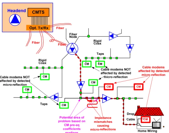
5.2.1 Micro-reflection Types

The following sections describe multiple scenarios in which micro-reflections may be generated within the HFC network.Micro-reflection Example 1 describes a case where there are HFC components whose low return loss (R) values are contributing to the micro-reflection source.Micro-reflection Example 2 describes a case where an HFC component whose isolation performance and an impedance mismatch are contributing to the micro-reflection source.Lastly, micro-reflection Example 3 describes a case where the micro-reflection impairments represent a combination of the two previous cases.Micro-reflection sources are not limited to the examples presented here. For more information about micro-reflections, refer to the tutorial section of this document.

5.2.1.1 Micro-reflection Example 1

This type of commonly experienced micro-reflection is exhibited when the upstream signal encounters impedance mismatches somewhere in its upstream path to the CMTS, causing redirection of a fraction of the signal’s energy back towards the CM. Once the redirected signal becomes incident on another impedance mismatch, it is then directed back toward the CMTS. Figure 1 illustrates an upstream signal, labeled Upstream Signal #2, on the cable originating between two reflection points, Γ1, and Γ2. However, the upstream signal may originate anywhere downstream from the first reflection point, Γ1, illustrated in the figure as Upstream Signal #1. The majority of the upstream signal passes through the impedance mismatch and continues toward the CMTS and is labeled Main Signal in the figure. A fraction of the upstream signal is reflected back towards the signal source at Γ1. This reflected signal encounters a second reflection point, Γ2 which reflects a fraction of the reflected signal energy back into the direction of the original signal, represented as Reflected Signal in Figure 1.

This general case describes the signal passing through two reflectors, neither of which is the CM itself. One technique to determine whether the CM is one of the reflectors is to add a 3 dB inline attenuator at the CM port (upstream output). If the micro-reflection magnitude is lessened by 6 dB or more, because of the reflected signal passing through the attenuator twice, then the CM is indeed one of the reflectors. If there is no significant change in micro-reflection magnitude, then the pair of reflectors lies remote to the CM location. This technique of adding attenuation would work equally well to isolate reflections elsewhere in the network, but it is much more difficult to install attenuation between line passives.

The reflected signal from Γ2 proceeds upstream and again encounters the reflection point Γ1. This causes yet another reflection back downstream, and the process repeats endlessly. (It is analogous to looking at one’s reflection in a mirror, when there is another mirror behind. There will be an endless sequence of images, each one progressively smaller.) Each passage between Γ1 and Γ2 is called a transit. The main micro-reflection echo results from the triple transit, up/down/up. The next echo is from the 5th-order transit up/down/up/down/up, and so on. This type of response, which goes on forever, is called infinite impulse response (IIR). It consists of a geometric series of echoes, separated by equal delays (equal to twice the propagation delay between the points Γ1 and Γ2), with each echo value smaller than the last (by the same ratio Γ1 Γ2 or, dB difference 10 log Γ1 + 10 log Γ2). The decaying micro-reflections may quickly be lost in the noise floor after two or three trips through the micro-reflection source. Conversely, the adaptive equalizer response, which is approximately the inverse of the channel response, will have only a single tap after the main tap for this case.

Though the reflector examples in Figure 1 are feeder taps, it should be noted that many devices can produce similar results, including damaged cables or corroded splices, which are often causes of micro-reflections as well.

Note that the delay between echoes equals twice the propagation delay between the two reflection points Γ1 and Γ2, so the distance between the two reflectors is known. However it does not relate how far along the plant these two

(21)

reflectors are, that is, the location of the impairment in the plant. To determine the location of the fault, additional information is necessary as described in Section 6.6, Fault Localization.

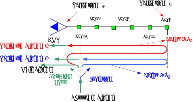
TAP23 AMP TAP17 TAP20 Reflected Signals Main Signal First Reflection Γ1 Second Reflection Γ2

Reflected Signal Attenuation Factor

ΓE = A Γ1Γ2e-jωt

TAP14

TAP11 TAP8

Roundtrip Attenuation & Delay A*e-jωT’ Upstream Signal # 1

Upstream Signal #2

Channel Impulse Response Representation

1 2 3 4 5 6 7 8 9 10 11 12 13 14 15 16 17 18 19 20 21 22 23 24 0 -10 -20 -30 -40 -50 Time Ma gni tu de (d B) MR = -10 dBc, 2T Main Tap

Figure 1 - Micro-reflection with multiple-transit echoes

5.2.1.2 Micro-reflection Example 2

The second type of micro-reflection may occur anywhere in the network, but its magnitude is most noticeable in CMs located off the highest value feeder taps. Figure 2 describes the upstream signal flow from a CM sending its upstream signal into the port of the 23 dB feeder tap. The intent of the plant design is that the primary path of upstream signal flow is toward the left of the page, toward the CMTS. Some signal energy may be reflected from the amplifier to the left of the 23 dB feeder tap, but this energy is usually insignificant because of good impedance matching of the amplifier.

The 23 dB feeder tap is a combination directional coupler and splitter meaning it directs the upstream signal in the upstream direction. The directivity of the feeder tap is not perfect. Some of the energy from the CM may be leaked towards the output connector. This is a function of the isolation of the feeder tap. Isolation is specified with all ports terminated, and cable industry field practice has often not adhered to terminating unused feeder tap ports. In addition, corrosion of the feeder tap can degrade its isolation performance.

If a 23 dB feeder tap has a tap-port-to-output-port isolation of only 38 dB, there would be two signal paths created, one with 23 dB attenuation, and one additional signal going the other direction with only 38 dB attenuation. If this additional signal meets a reflector downstream from the 23 feeder tap, the additional signal will be reflected back in the direction of the upstream signal and will be combined with the main signal at the 23 dB feeder tap where it originated. This micro-reflection is easily observed in cases where there is long un-tapped span of cable between the first feeder tap, the 23 dB feeder tap in this case, and low-value feeder taps with open terminations. All of these unterminated feeder tap ports create their own reflections. This condition usually creates multiple micro-reflections, and since there was an open port at the 11 dB feeder tap and another at the 8 dB feeder tap, there would be two different cable lengths resulting in two different micro-reflection delay characteristics.

This case is important to mention since the reflector, Γ1, is not in the tree of the devices between the CM and the CMTS, but includes devices that are downstream from the CM feeder tap location. This phenomenon, as mentioned earlier, is more noticeable at the high value feeder tap, because as the feeder tap value decreases, the amplitude difference between the desired signal and the micro-reflection increases. If both the 23 dB feeder tap and the 11 dB feeder tap had 35 dB tap-port-to-output-port isolation, there would be 12 dB greater separation between desired and the micro-reflection signal. Additionally, the 23 dB feeder tap location is near the amplifier followed by a long

(22)

length of cable, where the 11 dB feeder tap is found near the end of the cable so the cable length for the 11 dB feeder tap is shorter and the micro-reflection delay characteristic is correspondingly less.

This type of micro-reflection does not exhibit an unending IIR response, since the reflected energy from Tap 8 passes through Tap 23 relatively unimpeded and continues upstream. This type of response, which stops after a single echo, is called finite impulse response (FIR). The signature will show a single main echo without trailing echoes.

Conversely, the adaptive equalizer response, which is approximately the inverse of the channel response, will have a sequence of smaller and smaller taps for this case. This is because the equalizer internally generates additional echoes as it cancels the original echo in the signal. As it generates an echo, it must use another tap to cancel the new echo. This process goes on until the end of the equalizer tapped delay line is reached. Any remaining echo energy is uncompensated after this point, and results in reduced RxMER.

To summarize, a multiple-transit echo scenario (Example 1) has an unending sequence of decaying echoes in the channel response, and the corresponding adaptive equalizer response has a single echo. A single-reflection scenario (Example 2) has a single echo in its channel response, and the corresponding adaptive equalizer response has a decaying sequence of echoes continuing to the end of the equalizer tapped delay line.

Roundtrip Attenuation & Delay A*e-jωT’ TAP23

AMP

Reflected Signal Main Signal

First Reflection Γ1

Reflected Signal Attenuation Factor

ΓE = L*A Γ1e-jωt TAP11 TAP8 Upstream Signal Isolation Coupling Loss L = Isolation-Coupling Loss Other Possible Reflection Point

Channel Impulse Response Representation

1 2 3 4 5 6 7 8 9 10 11 12 13 14 15 16 17 18 19 20 21 22 23 24 0 -10 -20 -30 -40 -50 Time M agn itu de (dB) MR = -15 dBc, 4T Main Tap

Figure 2 - Micro-reflection with single impedance mismatch interface

5.2.1.3 Micro-reflection Example 3

Figure 3 represents a case that is a superposition of the previous cases described in Micro-reflection Example 1 and Micro-reflection Example 2. A reflective point exists if the amplifier has poor return loss. A fraction of the desired signal is reflected off the output of the amplifier, Γ1, and propagates downstream to the open connection at the end-of-line or an open feeder tap port, Γ2, where it reverses direction back towards the amplifier and rejoins the original signal at the feeder tap location.

If the amplifier and feeder tap are co-located or are very close together, there will little difference in micro-reflection delay characteristic between the previously described Micro-micro-reflection Example 1 and Micro-micro-reflection Example 2. In fact, they may add or cancel each other out.

However, if the amplifier is a pole span or more away from the feeder tap, there may be two different distinct micro-reflections created for the single unterminated feeder tap. These micro-micro-reflections are usually low in magnitude, 30 dB or more lower than the incident signal, but they can be numerous in a single amplifier-to-termination span.

(23)

It is conceivable that multiple micro-reflections may emanate from successive multiple passes through HFC components comprising the micro-reflection source. Cases in which only a single micro-reflection exists may be limited to laboratory simulation of the micro-reflection impairment and may not be practically encountered within the HFC network.

The cable industry has favored “capping” unused feeder tap ports rather than terminating the ports. Some operators will defend that position because it is claimed to reduce potential ingress sources. Indeed it is a tradeoff between craft integrity and good impedance matching practices, which causes more stress on the upstream adaptive equalizer.

**Delay 2*T**

1 TAP23

AMP

TAP17 TAP20

Reflected Signal #2

Main Signal

Reflection

Γ

1 TAP11 TAP8

Upstream Signal

Isolation

Coupling

Loss

Reflected Signal #1

Reflection

Γ

2

**Delay 2*T**

2

Figure 3 - Composite Micro-reflection resulting from Type 1 and Type 2 Micro-reflections

5.3 Pre-equalization Mechanism Enabled through DOCSIS Ranging

The upstream pre-equalization mechanism relies on the interactions of the DOCSIS ranging process in order to determine and adjust the CM equalization coefficients. The intent is for the CM to use its coefficients to pre-distort the upstream signal such that the pre-pre-distortion equals the approximate inverse of the upstream path distortion, so that as the pre-distorted upstream signal travels through the network it is corrected and arrives free of distortion at the upstream receiver at the CMTS.

The pre-equalization coefficients of the CM are the complex coefficients (F1 through F24) of the 24-tap linear transversal filter structure shown in Figure 4.

(24)

+

2 3 14 15

Input

z-1 _z-1 _z-1 _z-1 _z-1 _z-1 _z-1

+

. . . . . . F2 F1 F3 F4 F21 F22 F23 F24

Equalizer

Output

Figure 4 - Upstream Equalizer Structure

In this structure the blocks with z-1_{label represents delay elements, each of which in the DOCSIS 2.0 pre-equalizer} is the symbol period T (in DOCSIS 1.1 it can also represent delays equal to T/2 and T/4).

In the ranging process the CM sends a ranging request message (RNG-REQ) to the CMTS. The CMTS may use a known portion of this message, such as the preamble, as well as other known messages to determine the quality of the received signal, as well as to determine the adjustment the CM should make to its pre-equalization coefficients to better compensate the upstream distortion. In response to the RNG-REQ message, the CMTS sends a ranging response (RNG-RSP) message with a set of 24 coefficients and a parameter that indicates whether these coefficients are intended to result in a set or adjust operation by the CM. In the case of a set command, the CM will replace its existing coefficients with the ones sent by the CMTS. In the case of an adjust command, the CM convolves its coefficients with the ones sent by the CMTS to achieve the adjusted coefficients (Figure 5).

(25)

CMTS

CM

RNG-REQ

RNG-RSP

Freq. Adjust

Timing Adjust

Power Adjust

Transmit Eq. Adjust

Ranging Status

Calculates

PreEq.

Coefficients for

CM

Generates new

coefficients

based on the

ones sent by

CMTS

Amp.

Transmit Eq. Set

Figure 5 - CM-CMTS Ranging Interaction Enabling Pre-equalization Process

The CMTS may not be completely satisfied with the quality of the signal the CM is sending after the initial try. This is an iterative process which may take a few interactions before the coefficients are stable.

CMTS implementations use for the most part the transmit-equalization-adjust option to convey information. Only after the initial ranging request, one may see a CMTS send a transmit-equalization-set message to make sure that the CM initializes properly. In principle the CMTS could use this message when it needs to reset the coefficients. A CMTS that is completely satisfied with the values of the pre-equalization coefficients sends an adjust message where all coefficients are zero except for the pre-equalizer’s main tap coefficients, which has maximum or nominal value. This represents a Kronecker delta or impulse function, and any data set convolved with an impulse results in the original data set, which in this case is the CM pre-equalization coefficients, unchanged.

5.3.1 Pre-equalization Enabling Messages

As described previously, the two messages that are key in the ranging process are the range response (RNG-RSP) and range request (RNG-REQ) messages. The RNG-RSP message, which is generated by the CMTS in response to a RNG-REQ message, carries timing, frequency, power level, and equalization adjustment information as well as equalization set or load information and ranging status. This information is encoded following what is known as type-length-value (TLV) format. DOCSIS 1.1 pre-equalization coefficients are identified by type 04 and DOCSIS 2.0 or 3.0 by type 09. The RNG-RSP messages that the RNG-REQ messages correspond to are linked by the service ID or SID. SIDs identify upstream service flows. It may be that a CM has several SIDs. In that case a CM will get ranging information through each of the SIDs it has. For example, if a CM has a SID that is used for telephony service and one that is used for data service, there will be two parallel ranging processes within a single CM. In addition to the SID, the RNG-RSP message payload also carries the upstream channel ID. Figure 6 shows the structure of the RNG-RSP message.

(26)

MAC Header 6 bytes +EHDR MAC mgmt msg 24-1522 bytes Destination 6 bytes Source 6 bytes msgLE N 2 bytes DSAP 1 byte SSAP 1 byte 1 bytectrl Ver. 1 byte type 1 byte 4 bytesCRC RSVD 1 byte management message payload

Ranging Response (RNG-RSP) TLV Encoded _Information

SID from corresp. RNG-REQ

2 bytes

Up. Ch. ID 1 byte Figure 6 - Range Response Message Format

The RNG-REQ message is generated by the CM and sent to the CMTS. The RNG-REQ is used as the reference to determine whether the CM signal needs any adjustment. These adjustments could be in frequency, power level, timing offset, and distortion. Once the CMTS receives the RNG-REQ message it uses a known portion of this message as the reference of what the signal should look like. Typically that known portion of the message is the preamble. If the CM is not finished implementing the changes the CMTS is asking for, the CM includes in the RNG-REQ message a ranging status indicating whether or not the ranging changes are still pending. This is the “pending till complete” field in the RNG-REQ message payload. The RNG-REQ message also carries a downstream channel ID that associates the upstream being used with a downstream channel. Figure 7 shows the structure of the RNG-REQ message.

(27)

PMD Overhead DOCSIS Payload Ramp-Up Next Burst Preamble Preamble 0-1024 bits (0-128 Bytes) FEC Info/Parity Overhead 18-255 bytes (10-25% of user data) PMD Overhead Ramp-Down Guard Time 5-255 symbols 1.25-63.75 bytes QPSK 2.5-127.5 bytes 16QAM Zero-Fill if necessary Integer Number of Minislots Mini-Slot Boundary of previous Burst Destination

6 bytes 6 bytesSource

msgLE N 2 bytes DSAP 1 byte SSAP 1 byte 1 bytectrl Ver. 1 byte type

1 byte RSVD1 byte 4 bytesCRC management

message payload

Ranging Request (RNG-REQ) MAC Header 6 bytes +EHDR MAC mgmt msg 24-1522 bytes DS Ch. ID 1 byte Pending Till Complete 1 byte SID 2 bytes

Figure 7 - Range Request Message Format

5.3.2 CM and CMTS Equalization Information

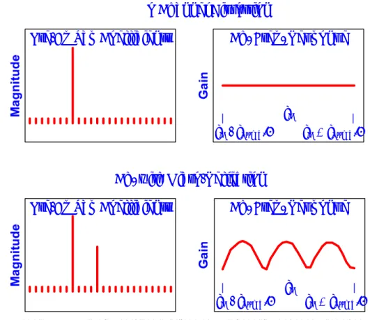
The pre-equalization coefficients are loaded into the adaptive pre-equalizer in the CM, which is used to compensate for upstream linear distortion(s). Hence the CM pre-equalization data indirectly describes the distortion in the plant for which it compensates. The pre-equalizer response is approximately the inverse or opposite response of the plant. The pre-equalization coefficients provide detailed characteristics of the channel distortion, although the coefficients do not directly indicate the level of micro-reflections. Assuming negligible group delay distortion and a single micro-reflection, a quick estimate of micro-reflection level can sometimes be obtained using the energy in the adaptive equalizer’s non-main taps. In general, an elaborate analysis is required to uniquely resolve micro-reflection level/delay signature characteristics. An upstream channel that exhibits no distortion has all the energy concentrated in the adaptive equalizer main tap while one that exhibits distortion also has energy in taps other than the main tap (Figure 8).

(28)

f

C

+ f

Symb

/2

f

C

- f

Symb

/2

f

C

f

C

+ f

Symb

/2

f

C

- f

Symb

/2

f

C

Ch. Freq. Response

Pre-Eq Tap Coefficients

No Channel Distortion

Ch. with Micro-Reflection

Figure 8 - CM Pre-eq Coefficients Values and Frequency Response Scenarios

The pre-equalization data which the CMTS continues to send to the CM indicates how successful a CM has been in compensating for the distortion by showing what is left to compensate to achieve ideal reception. Ideally and typically, the CM starts with no compensation and after a few ranging intervals, achieves a steady state where the CM compensates for all the distortion. At that point the CMTS pre-equalization data exhibits a flat response indicating that further compensation is not required (Figure 9).

(29)

f

C

+ f

Symb

/2

f

C

- f

Symb

/2

f

C

f

C

+ f

Symb

/2

f

C

- f

Symb

/2

f

C

Ch. Compensation

Completed

Ch. Compensation Still

Needed

Pre-Eq Tap Coeff. Settled

Initial Pre-Eq Tap Coeff.

Initial CMTS State

CMTS State after Settling

Figure 9 - CMTS CM Pre-equalization Coefficients Values and Frequency Response Scenarios

The upstream CM equalization data collected by the CMTS is analyzed to verify that any plant distortion has been compensated. There is the possibility of a distortion being so severe (e.g., a micro-reflection having a very long delay) that the pre-equalization process would not be able to fully compensate for it. These scenarios are rare in current HFC architectures, but if this does occur, one must be aware that an impairment identification process using only CM pre-equalization data will not yield accurate results.

5.4 Upstream Pre-equalization in DOCSIS 1.0, DOCSIS 1.1 and DOCSIS 2.0

Upstream pre-equalization in DOCSIS 1.0 was left as optional and the equalization process between CMTS and CM was not defined in sufficient detail. An unexpected result occurred when DOCSIS 1.1 and 2.0 were introduced with a well defined process. A few 1.0 CMs that implemented pre-equalization exhibited erratic behavior in the presence of downstream RNG-RSP messages that were generated by 1.1 or 2.0 CMTSs. For quite some time operators have not been motivated to turn pre-equalization on, in part because the demand for capacity and spectrum availability have not been significant enough to warrant the use of wider channels, higher order modulations, or frequencies near the edges of the upstream spectrum where linear distortion occurs.

Some 1.0 CMs exhibiting the problem have been successfully upgraded with firmware that corrects this issue. Unfortunately it has not been possible to correct this issue on all affected CMs. To support reliable use of upstream pre-equalization, operators have been replacing 1.0 CMs having known issues.

5.4.1 DOCSIS 1.1 Pre-equalization Considerations

The percentage of DOCSIS 1.1 CMs deployed is still significant enough not to take advantage of the

How To Understand And Understand The Power Of A Powerline Microscope

DOCSIS

®

Best Practices and Guidelines

Proactive Network Maintenance Using

Pre-equalization

CM-GL-PNMP-V02-110623

RELEASED

Document Status Sheet

Key to Document Status Codes

Trademarks

Contents

Figures

Tables

1 SCOPE

1.1

Introduction and Purpose

2 REFERENCES

2.1

Informative References

2.2

Reference Acquisition

3 TERMS

AND

DEFINITIONS

4 ABBREVIATIONS AND ACRONYMS

5 BACKGROUND

5.1

Reactive versus Proactive Network Maintenance

5.2

Linear Impairments





d

d

GroupDelay









Delay 2*T

AMP

Reflected Signal #2

Main Signal

Reflection

Γ

Upstream Signal

Isolation

Coupling

Loss

Reflected Signal #1

Reflection

Γ

Delay 2*T

5.3

Pre-equalization Mechanism Enabled through DOCSIS Ranging

+

Input

+

+

+

+

+

+

Equalizer

Output

CMTS

CM

RNG-REQ

RNG-RSP

Freq. Adjust

Timing Adjust

Power Adjust

Transmit Eq. Adjust

Ranging Status

Calculates

PreEq.

Coefficients for

CM

Generates new

**Delay 2*T**

**Delay 2*T**