eigenfunctions
Thomas Willer
To cite this version:
Thomas Willer. Optimal bounds for inverse problems with Jacobi-type eigenfunctions. Statis-tica Sinica, Taipei : Institute of StatisStatis-tical Science, Academia Sinica, 2009, 19 (2), pp.785-800. <hal-00133830v2>
HAL Id: hal-00133830
https://hal.archives-ouvertes.fr/hal-00133830v2
Submitted on 21 Oct 2013HAL is a multi-disciplinary open access archive for the deposit and dissemination of sci-entific research documents, whether they are pub-lished or not. The documents may come from teaching and research institutions in France or abroad, or from public or private research centers.
L’archive ouverte pluridisciplinaire HAL, est destin´ee au d´epˆot et `a la diffusion de documents scientifiques de niveau recherche, publi´es ou non, ´emanant des ´etablissements d’enseignement et de recherche fran¸cais ou ´etrangers, des laboratoires publics ou priv´es.
OPTIMAL BOUNDS FOR INVERSE PROBLEMS WITH JACOBI-TYPE EIGENFUNCTIONS
Thomas Willer
Universit´e de Provence
Abstract: We consider inverse problems where one wishes to recover an unknown function from the observation of a transformation of it by a linear operator, cor-rupted by an additive Gaussian white noise perturbation. We assume that the operator admits a singular value decomposition where the eigenvalues decay in a polynomial way, and where Jacobi polynomials appear as eigenfunctions. This in-cludes, as an application, the well known Wicksell’s problem. We establish asymp-totic lower bounds for the minimax risk in a wide framework (i.e. with(Lp)1<p<∞
losses and Besov-like regularity spaces), which show that the estimator of Kerky-acharian, Picard, Petrushev, and Willer (2007) is quasi-optimal, and thus yield the minimax rates. We also establish some new results on the needlets introduced by Petrushev and Xu (2005) which appear as essential tools in this setting. Lastly we discuss the interest of the results concerning the treatment of inverse problems by wavelet procedures.
Key words and phrases: statistical inverse problems, minimax estimation, second-generation wavelets.
1. Motivation
We consider the problem of recovering a functionffrom a blurred and noisy version Y:
∀v∈V, Y(v) = (Kf, v)V +ξ(v),
where K is a linear operator between two Hilbert spaces: K : U 7→ V, ξ is a Gaussian white noise on V, and forH a Hilbert space andh1, h2 ∈H,(h1, h2)H denotes the scalar product inHbetweenh1 andh2. We assume thatfbelongs to
U=L2([−1, 1], µ(x)dx),with µ(x) = (1−x)α(1+x)β, α, β >−1/2, and that
Kadmits a singular value decomposition (SVD), i.e. there exists an orthonormal basis (called SVD basis) formed by the eigenfunctions of the self-adjoint oper-ator K∗K (where K∗ is the adjoint of K). Moreover we assume that this SVD
basis consists of the classical Jacobi polynomials of type (α, β), and that the corresponding sequence of eigenvalues tend to zero at a polynomial rate. We will name such problems ”Jacobi-type inverse problems”.
The main motivation of this article is to establish asymptotic lower bounds for the minimax risk in a wide framework, consideringLp([−1, 1], µ)losses, for all
1 < p <∞, and a Besov-like regularity space. This combined with the result of Kerkyacharian, Picard, Petrushev, and Willer (2007) (where upper bounds are provided) shows some new rate phenomenom for inverse problems.
1.1 What are the interests of the results?
The most popular technique for the treatment of inverse problems is prob-ably singular value decomposition estimation, where the unknown function is expanded in the SVD basis, and the corresponding coefficients are estimated thanks toY. Such techniques are very attractive theoretically and can be shown to be asymptotically minimax in many situations (see e.g. Mathe and Pereverzev (2003), Cavalier and Tsybakov (2002), Cavalier, Golubev, Picard, and Tsybakov (2002), Tsybakov (2000), Goldenshluger and Pereverzev (2003)). However there are limitations in the minimax framework, in particular such estimators gener-ally cannot estimate functions exhibiting inhomogeneous regularity. To avoid this problem, several wavelet methods have been introduced during the last decade (for example Donoho (1995) and Abramovich and Silverman (1998)), which are minimax over wide sets of target functions, for example Besov spaces. Never-theless such methods apply only to a category of inverse problems where the operator is well adapted to the structure of ”first generation” wavelets, which are built from a Fourier analysis perspective. Thus many wavelet estimators are available whenever the operator displays some convolution structure (see for instance Pensky and Vidakovic (1999), Fan and Koo (2002), Kalifa and Mallat (2003)).
The main interest of our results is to grapple with quite different inverse problems, where the operator displays a polynomial structure. Then classical wavelets cannot be used, and new estimation techniques were given by Kerky-acharian, Picard, Petrushev, and Willer (2007): one uses new wavelets built upon polynomials (termed needlets, and introduced by Petrushev and Xu (2005)) to
develop the ”NEEDD” estimator, and new spaces (which appear as an adapta-tion of the classical Besov spaces) to assess its performances. Here we establish a lower bound for the minimax risk, which matches with the rates of conver-gence of NEEDD (up to log factors). Consequently we obtain the minimax rates in all the Jacobi-type inverse problems, and we prove the quasi optimality of NEEDD. Note also that the results are established for all Lp([−1, 1], µ) losses whereas in most other works cited previously, only the case p = 2 is consid-ered, with one exception: for the deconvolution problem in a periodic setting, Johnstone, Kerkyacharian, Picard, and Raimondo (2004) combined with Willer (2005) established the minimax rates for all Lp([0, 1], dx) losses and over Besov
spaces. We will draw a parallel between those rates and the ones obtained here: we exhibit elbow effects, and we show that the rates in the deconvolution model appear as a critical case of the rates in the Jacobi-type model. Moreover, we also give an application of our results to Wicksell’s problem, which satisfies the required assumptions on the operator. This problem concerns the recovery of the density of the radii of spherical particles, when a sample of planar cuts is given, and has many applications in medecine and in biology.
In this paper, we have only considered standard inverse problems, where the operator is known. Recently, SVD or wavelet estimators have also been devel-oped for noisy operators (see e.g. Efromovich and Koltchinskii (2001), Cavalier and Hentgartner (2005), Cavalier and Raimondo (2007) or Hoffmann and Reiss (2007)), and it may be interesting in the future to expand our results to that setting.
1.2 Which difficulties are met to prove the results?
The main idea behind NEEDD is to decompose the problem by using a family of functions (the needlets) which in some sense ”both quasi-diagonalizes the operatorKand the prior information onf” (to use Donoho’s terms in Donoho (1995)). In the lower bound problem treated here, a similar problem arises, as we need a family of functions {fλ, λ∈Λ}⊂Urepresentative of the difficulties of estimation inside the regularity space considered for the risk. This means that the functions fλ must be chosen such that:
• at the same time the distributions of the associated processesY are close to one another (in a Kullback sense, for example).
A natural way to build such hypotheses is to use functions which enjoy localiza-tion properties, and whose images byKcan be easily studied, and thus here again needlets are an essential tool. The hypotheses are built as linear combinations of such functions, with some parameters left free, which we adjust optimally with respect to the two constraints cited above. Then the minimal Lp(µ) distance between the hypotheses yields the lower bound on the whole regularity space. This approach combining wavelets and lower bound techniques is classical (see Tsybakov 2004), but the main tool used here - the needlets - is quite unusual: their properties are still not thoroughly known, and in several ways they do not behave like classical wavelets. Thus in section 5.4 we give a brief list of needlet properties used to prove our results, some of which are established here. We show that, in particular, the non orthogonality of the needlets and the heterogeneity of theirLp(µ)norms makes the lower bound problem more difficult than in other inverse problems, such as deconvolution for example (for which a proof using the classical Meyer wavelets can be found in Willer (2005)).
The paper is organized as follows. In section 2 we describe the model and state the main result, in section3 we give an application to the Wicksell’s prob-lem, and in section 4we discuss the interests of the results among the literature on inverse problems. Lastly in section 5 we give the proof of the main theo-rem, along with a description of the needlets where some new properties are established.
2. Main result
2.1 Model and assumptions
We are interested in nonparametric inverse problems in white noise, with a polynomial structure of the operator. We define this framework as follows. Letf
be an unknown function belonging to the Hilbert space U=L2([−1, 1], µ(x)dx),
with µ(x) = (1−x)α(1+x)β, α, β >−1/2. The estimation problem consists in recovering a good approximation of the functionffrom the observation of the random variableY corresponding to a blurred and noisy version off:
Blurring effect: Let I = [a, b] or I = [a, b[, with −∞ < a < b ≤ ∞, and
λ:I7→R∗+ a continuous function. We setV=L2(I, λ(x)dx). LetK:U7→V be a linear operator satisfying the two following conditions. First assumeK∗K(where
K∗ denotes the adjoint ofK) is diagonalizable, with a countable set of eigenvalues (denoted(b2k)k∈N) which are strictly positive and decrease at a polynomial rate
for some ill posedness coefficient ν > 0 (for two positive sequences (uk) and (vk), the notation uk vk means that there exist 0 < c1 ≤ c2 < ∞ such that
c1vk ≤uk ≤c2vk):
∀k∈N∗, bkk−ν.
Secondly, assume that the classical Jacobi polynomials normalized inU (we de-note byPkα,βor simplyPk the polynomial of degreek) appear as an orthonormal basis of eigenfunctions of K∗K. So Pk is the polynomial of degree k such that
R1
−1PkPldµ=δk,l, and we have:
∀k∈N, K∗KPk=b2kPk.
Noise effect: > 0is deterministic, andξ is a Gaussian white noise onV, i.e.:
∀v, w∈V, ξ(v)∼N(0,kvk2 V), E[ξ(v)ξ(w)] = (v, w)V. 2.2 Minimax rates
The aim of the paper is to establish the asymptotic minimax rates (when
→ 0) for inverse problems described above, in a wide framework, i.e. for numerous choices of functions f and of measures of estimation errors. For the latter, we consider all Lp(µ) losses (for any 1 < p < +∞) defined by: ∀u∈ U, kukLp(µ) = [
R1
−1|u(x)|
pdµ(x)]p1. Concerning the target functions, we introduce
spaces Bsπ,r(M) below, which appear as an adaptation of the classical Besov spaces. Let(ψj,η)j≥0, η∈Zj denote the tight frame of needlets described in section
5.4. For anyf∈U, we have the following decomposition:
f=X
j≥0
X
η∈Zj
βjηψjη, whereβjη= (f, ψjη)U.
Then for π≥1, s≥1/π,r≥1,M > 0 we define:
Bsπ,r(M) ={f∈U | k(2js(X
η∈Zj
Ifψj,η were a classical wavelet, thenBs
π,r would correpsond to Besov spaces (see
e.g. H¨ardle, Kerkyacharian, Picard, and Tsybakov (1998)), which are very gen-eral regularity spaces including as particular cases Sobolev and Holder spaces, and which can be described very simply, thanks to any regular enough wavelet ba-sis. Such spaces are widely used to study the theoretical performances of wavelet estimators in appropriate inverse problems. However here Bsπ,r correspond to new spaces, characterized by needlets, and appear as a natural alternative to the classical Besov spaces when the inverse problem does no longer possess a convo-lution structure, but a polynomial structure. Details on the space in this case can be found in Narcowich, Petrushev, and Ward (2006) and in the appendix of Kerkyacharian, Picard, Petrushev, and Willer (2007).
We are interested in the minimax risk defined by:
R(Bsπ,r(M),Lp(µ)) :=inf ^ f sup f∈Bs π,r(M) Ef(kf^−fkpLp(µ)),
where the infimum is taken over all σ(Y(t))t≥0−measurable estimators f^. The
results of Kerkyacharian, Picard, Petrushev, and Willer (2007), concerning the rates of convergence of the NEEDD estimator, give immediately an upper bound for the risk. This is Theorem 1, where we recall that ν > 0is a rate of decay of the eigenvalues of the operator (bkk−ν), and thatα, β >−12 are parameters characterizingU.
Theorem 1. For all 1 < p < ∞, π ≥ 1, r ≥1 and s >maxγ∈{α,β}{12 −2(γ+
1)(12 −π1)∨2(γ+1)(π1 − p1)∨0} there exists C > 0 such that:
R(Bsπ,r(M),Lp(µ))≤C[log(1/)]p+1[
p
log(1/)]ζp,
where ζ=min{ζ(s), ζ(s, α), ζ(s, β)} with:
ζ(s) = s
s+ν+ 12, ζ(s, γ) =
s−2(1+γ)(π1 − p1)
s+ν+2(1+γ)(12 − π1).
The main purpose of the paper is to prove that these rates coincide with the rates of the minimax risk up to log factors. We will establish the following theorem:
Theorem 2. For all 1 < p <∞, π≥ 1, r≥ 1 and s ≥1/π there exists C > 0
such that:
where ζ=min{ζ(s), ζ(s, α), ζ(s, β)} with:
ζ(s) = s
s+ν+ 12, ζ(s, γ) =
s−2(1+γ)(π1 − p1)
s+ν+2(1+γ)(12 − π1).
Note that the exact logarithmic factors of the minimax risk are not estab-lished yet. In this paper we have focused only on the main rateζ, so our results
prove that NEEDD is ”quasi optimal” in the Jacobi-type models. 3. Application to the Wicksell’s problem
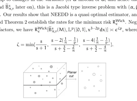
The Jacobi-type inverse models considered in this paper find applications in practice, in particular with the well known Wicksell’s problem (Wicksell (1925)), which corresponds to the following situation. Suppose a population of spheres is embedded in a medium, with radii that may be assumed to be drawn indepen-dently from a densityf. A random plane slice is taken through the medium, and some spheres are intersected by it. They furnish circles, the radii of which yield the points of observation Y1, . . . , Yn, as illustrated in Figure 3.1. The unfolding problem is to determine the density of the spheres radii from the observed circle radii. This problem arises in medicine, where the spheres might be tumors in an animal’s liver (Nychka, Wahba, Goldfarb, and Pugh (1984)), as well as in nu-merous other contexts (biological, engineering, etc.) see for instance Cruz-Orive (1983).
If one uses the Lebesgue measure, then by a conditioning argument (see Wicksell (1925)) and under some assumptions, the density of the circles radii is:
∀y∈[0, 1], K0f(y) =yRy1(x2−y2)−1/2f(x)dx (up to a constant). However few articles use this precise formulation of the problem. In the sequel we adopt the version proposed by Johnstone and Silverman (1991) who replaced the Lebesgue measure by two weighted measures. So we observe Y following model (2.1) with
K:Ue 7→V given by: e U=L2([0, 1],eµ(x)dx), eµ(x) = (4x)−1, V=L2([0, 1[, λ(y)dy), λ(y) =4π−1(1−y2)1/2, Kf(y) = π4y(1−y2)−1/2Ry1(x2−y2)−1/2f(x)dµe(x).
Johnstone and Silverman (1991) show thatK∗Kadmits the following root eigen-values and eigenfunctions: bk= 16π(1+k)−1/2,
e
Pk(x) =4(k+1)1/2x2P0,1 k (2x2−
1). Thus up to changes in the variables (cf Ue instead of U, and hence the nota-tionseP and Besπ,r later on), this is a Jacobi type inverse problem with(α, β, ν) = (0, 1, 1/2). Our results show that NEEDD is a quasi optimal estimator, and The-orem 1 and TheThe-orem 2 establish the rates for the minimax riskRWick . Neglecting log(1/) factors, we haveRWick [Besπ,r(M),Lp([0, 1], x3−2pdx)]ζp,where:
ζ=min{ s s+1, s−2(π1 − p1) s+ 32− π2 , s−4(1π− 1p) s+ 52 − π4 }.
Figure 3.1: Wicksell’s problem: observation of radii of disks after a planar cut of spheres
Thus we find rates which are new in the literature on Wicksell’s problem, but of course several comments need to be done. First we used a transformation, initiated by Johnstone and Silverman (1991), of the original Wicksell problem. Other statistical results are available, but stated in yet another version of the problem, where one considers the squared radii of circles and spheres. Then a thorough minimax study can be found in Golubev and Levit (1998) for the esti-mation of the corresponding distribution function, and in Antoniadis, Fan, and Gijbels (2001) convergence rates are established for a wavelet density estimator, but only in L2([0, 1], dx) norm and over particular Besov spaces. Secondly we
assumed that the random perturbation is a Gaussian white noise on the spaceV
introduced above, and not a density perturbation as in the original problem. So here we add to the variety of theoretical results on Wicksell: we draw a complete picture of the problem in a minimax perspective, but by using a rather unusual representation. Work still needs to be done to extend our results to a more prac-tical setting: research in that direction is initiated in Chapter 5 of Willer (2006), but a more thorough investigation is under study.
4. Discussion
In the literature on statistical inverse problems, there are few results in a minimax framework as general as the one considered in this paper. Usually, only the L2 case is considered, and under the polynomial decay assumption of the eigenvalues, the rate ζ= s+νs+1/2 (named ”regular” rate) appears frequently (see Cavalier and Tsybakov (2002)). For more general Lp losses, only the case of deconvolution in a periodic setting (up to our knowledge) has been studied in Johnstone, Kerkyacharian, Picard, and Raimondo (2004) and Willer (2005), and elbow effects appear, with a second rate named ”sparse”. It is interesting to draw a parallel between such a problem, where classical wavelets are widely used tools, and polynomial type problems, which require needlets.
For the deconvolution problem, minimax rates have been established for all
Lp([0, 1], dx) losses (1 < p < ∞) and over balls of a Besov space characterized by parameters π ≥1, s ≥ 1/π, r ≥ 1 as above. Then the rates are given as in Theorem 1 and 2 (up to the logarithmic factors) with ζ replaced by:
ζ=min{ζregular := s
s+ν+1/2, ζsparse:=
s−1/π+1/p s+ν+1/2−1/π}.
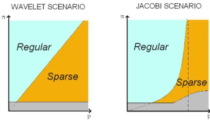
Then the deconvolution setting appears as a critical case of the Jacobi setting, if we set α = β = −12. More generally if we set α = β > −12 we can draw the cartography of the regular and sparse zones with respect to(p, π) (see figure 4.2), as was done in H¨ardle, Kerkyacharian, Picard, and Tsybakov (1998) in the direct observation case. In the deconvolution case (i.e. the ”wavelet scenario”) the separation between the zones is linear, whereas in the ”Jacobi scenario” the critical case is more complicated. So in that scenario we find new rates, and note that this novelty is not an artifact stemming from the weights on the space, since in the Lebesgue case the rates for the Jacobi scenario (i.e. α= β = 0) do not coincide with those of the wavelet scenario. Thus the origin of the differences lies in the polynomial structure of the inverse problems, in opposition to the convolution structure of the problems usually treated by first generation wavelet methods.
These results illustrate the fact that the limitations met by classical wavelets in inverse problem theory, concerning the type of operators involved, can be circumvented by using new wavelet constructions such as needlets. Similarly
other second generation wavelets, meaning wavelets which do not rely on Fourier type constructions, may help to break new ground in statistical inverse problems.
Figure 4.2: Cartography of the regular and sparse zones with respect to(p, π)in the deconvolution case (left) and in the Jacobi case ifα=β=0(right)
5. Proofs
5.1 General scheme of the proof
The proof of Theorem 2 requires well known methods for minimax lower bounds, as available in Tsybakov (2004), combined with new tools (i.e. needlets). We use Theorem 5.2 in Tsybakov (2004), which involves the Kullback-Leibler divergenceK(P, Q) between two probability measuresP and Q, defined by:
K(P, Q) =
R
ln(dQdP)dP, ifP Q; +∞, otherwise.
Changing the notations, and replacing slightly the conditions so as to include the case m =1 (the result remains true using τ =1/√m+1 instead of τ = 1/√m
in the proof), this theorem states that:
Theorem 3. Assume there exist m+1 functions f0, . . . , fm (with m≥1) satis-fying the three following conditions:
• Condition (i): for alli∈{0, 1, . . . , m},fi∈Bsπ,r(M),
• Condition (ii): for all i6=j, kfi−fjkpp≥2δ for some δ > 0,
θlog(M+1), where 0 < θ < 18 and Pf denotes the probability distribution of the process Y under the hypothesis f.
Then inff^supf∈Bs
π,r(M)Pf(k
^
f−fkpp ≥ δ) ≥ π0, where π0 is a positive universal
constant.
Let us precise condition (iii’) in model 2.1. Let I = [a, b] (the case I = [a, b[ is similar). If we define the variables Ye(w) = Y(w(.− a)/
p
λ(.)) and e
ξ(w) = ξ(w(.−a)/pλ(.)) for all w ∈ Ve = L2([0, b−a], dx) then model 2.1 is equivalent to: Ye(w) = (Kf(.+a)
p
λ(.+a), w)
e
V +eξ(w), which is equivalent
to the stochastic equation: ∀t ∈ [0, b−a], dYet = Kf(.+a) p
λ(.+a) +dWt
where (Wt)t≥0 denotes the standard Wiener process. Then using Girsanov’s
formula, for all f, g ∈ U, Pf is absolutely continuous with respect to Pg, and
under the hypothesis g the likelihood ratio Λ(f, g) := dPf
dPg(Y) is distributed as: logΛ(f, g)∼N(−21kK(f−g)k2 V,k K(f−g) kV).Thus K(Pf, Pg) =Efln(Λ(f, g)) = −Eflog(Λ(g, f)) = 1 2k K(f−g) k 2 V.
Then condition (iii’) can be replaced by the sufficient condition (iii):
Condition (iii): f0 = 0 and for all i ∈ {1, . . . , m}, kKfik2
V ≤ θlog(M+1)2
where0 < θ < 14.
We use Theorem 3 by building several sets of hypotheses{fi, i=0, 1, . . . , m}
satisfying the three conditions. Then using Chebychev’s inequality we have: inf ^ f sup f∈Bs π,r(M) Efkf^−fkpp≥π0δ.
With an appropriate choice of three sets {fi, i = 0, 1, . . . , m} depending on the
level of noise ,δ yields the three expected rates. We detail the sparse cases in section 5.2 and then the regular case in 5.3. Throughout these two sections, we use many (old or new) preliminary results on the needlets, all of which are given in section 5.4.
5.2 Sparse cases
The sparse rates µ(α)andµ(β)are obtained respectively by applying Theo-rem 3 to the following sets of functions: {f0=0, f1 =γψj0,η1},and{f0 =0, f1 =
γψj1,η
2j1},for some parametersγ,j0 andj1 chosen so as to satisfy conditions (i)
to (iii). We detail only the proof for µ(α) (the proof forµ(β) is similar).
Condition (i) is satisfied if uj := 2js(
P
η∈Zj|hf1, ψj,ηi|
πkψ
j,ηkππ)1/π belongs to
lr(M), where f1 = γψj0,η1. Using the first part of Lemma 1, uj = 0 whenever
|j−j0|≥2. So in the sequel we assume thatj∈{j0−1, j0, j0+1}, and thelrnorm of(uj) is bounded by a constantM(independent ofγ > 0andj0) if for instance
uj ≤ 3−1rM. We have: uπ j = 2jπsγπ P η∈Zj|hψj0,η1, ψj,ηi| πkψ j,ηkππ ≤ c(I1 +I2),
with, using the bound of Theorem 6:
I1=2j[πs+(π−2)(α+1)]γπ 2Xj−1 k=1 |hψj0,η1, ψj,ηi|πk−(π−2)(α+1/2), I2=2j[πs+(π−2)(β+1)]γπ 2j X k=2j−1+1 |hψj0,η1, ψj,ηi|π(2j−k+1)−(π−2)(β+1/2).
Using the second part of Lemma 1, we have for any ζ: |hψj0,η1, ψj,ηki| ≤ ck1ζ.
Thus choosing any ζ > −(π−2)(απ+1/2)+1, we obtain: I1 ≤ c2j[πs+(π−2)(α+1)]γπ.
Moreover P2kj=−11 (2j−k+1)−(kζππ−2)(β+1/2) ≤ c2−ζπj2j[1−(π−2)(β+1/2)]+, so for a large
enoughζ: I2 ≤c2j(πs+(π−2)(β+1)−ζπ+[1−(π−2)(β+1/2)]+)γπ ≤cI
1.Thus we have for
all j∈{j0−1, j0, j0+1}: uπj ≤c2j0[πs+(π−2)(α+1)]γπ,and condition (i) is satisfied
if, for a small enoughc depending onM:
γ≤c2−j0[s+(1−π2)(α+1)].
Condition (ii), using theorem 6, is fulfilled with: δγp2j0(p−2)(α+1).
Condition (iii) is satisfied if: RI(K(γψj0,η1 )(t))2dλ(t) ≤C. We have ψj0,η(x) =
P2j−1 l=2j−2+1cj,η,lPl(x) andK∗KPl=b2lPl,thus: kK(ψj0,η1)k 2 V = X l [blcj,η,l]2 2−2νj0 X l [cj,η,l]2 =2−2νj0kψj0,η1k 2 U≤C2−2νj0.
In view of the three conditions, we set γ = c2νj0 with a small enough c,
and 2j0
− 1
s+ν+(1−2π)(α+1). Then δ
p[s+2(1p−π1)(α+1)]
s+ν+(1−π2)(α+1) gives the sparse lower
bound.
5.3 Regular case
Letmbe an integer such that2m≥n2, wheren2is the integer from Theorem
7 in the case p= 2. For some parametersγ and j0 ≥m+1 chosen further, we
consider for ε∈{0, 1}2j0−m−1 the22j0−m−1 functions:
fε =γ
2j0X−m−1 k=1
εkkδψj0,η2mk,
for some δ satisfying: δ > max[1, α+1/2,(1− π2)(α+ 12) − 1π]. We only keep some of these functions. By Varshamov-Gilbert theorem (see for instance Tsy-bakov (2004)), there exists a subset Ej0 = {ε0, . . . , εTj0} of {0, 1}2j0−m−1 and two constantsc > 0,ρ > 0such that∀0≤u < v≤Tj0:
2j0−m−1 X k=1 |εuk −εvk|≥c2j0, T j0 ≥exp(ρ2 j0) and f ε0 =0.
In the sequel we consider the set{fε, ε∈Ej0}.
Condition (i): for ε ∈ Ej0, let uj := 2
js(P
η∈Zj|hf, ψj,ηi|
πkψ
j,ηkππ)1/π. Once
again uj =0whenever |j−j0|≥2. Now let j∈{j0−1, j0, j0+1}. Then we have:
uπj ≤c(I1+I2),with: I1 = 2j[πs+(π−2)(α+1)]γπ 2j−1 X k=1 k−(π−2)(α+1/2)( 2j0−1 X l=1 lδ|hψj0,ηl, ψj,ηki|) π, I2 = 2j[πs+(π−2)(β+1)]γπ 2j X k=2j−1+1 (2j−k+1)−(π−2)(β+1/2)( 2Xj0−1 l=1 lδ|hψj0,ηl, ψj,ηki|)π.
Using Lemma 1 with someζgiven later, we have|hψj0,ηl, ψj,ηki|≤c
1
(1+|l−2j0−jk|)ζ.
Then, forx∈R, letbxc denote the largest integer smaller than x. We have:
X l≤b2j0−jkc lδ (1+|l−2j0−jk|)ζ ≤ck δ X l≤b2j0−jkc 1 (1+b2j0−jkc−l)ζ ≤ck δX l≥1 1 lζ ≤ck δ,
for a large enoughζ. Moreover: X l≥b2j0−jkc+1 lδ (1+|l−2j0−jk|)ζ ≤ X l≥b2j0−jkc+1 lδ (l−b2j0−jkc)ζ = X l≥1 (l+b2j0−jKc)δ lζ ≤cX l≥1 lδ+b2j0−jkcδ lζ ≤Ck δ,
for ζ large enough. To obtain the last line, we used the fact that δ ≥ 1. Thus
P2j0−1 l=1 lδ (1+|l−2j0−jk|)ζ ≤ck δ, and: I1 ≤c2j[πs+(π−2)(α+1)]γπ 2j−1 X k=1 k−(π−2)(α+1/2)kδπ =c2j[s+δ+12]γ.
For I2 remark that for any k ∈ {2j−1 +1, . . . , 2j} and any l ∈ {1, . . . , 2j0−1},
we have: |2kj − 2lj0| = 2kj − 2j0l ≥ |2 j−k
2j − 2lj0|. So for such a k, as previously:
P2j0−1 l=1 l δ (1+|l−2j0−jk|)ζ ≤ P2j0−1 l=1 l δ (1+|l−2j0−j(2j−k)|)ζ ≤c(2 j−k)δ, and: I2 ≤c2j[πs+(π−2)(β+1)]γπ 2j X k=2j−1+1 (2j−k+1)−(π−2)(β+1/2)(2j−k+1)δπ =c2j[s+δ+12]γ.
Finally we haveuj≤c2j[s+δ+12]γsofεbelongs toBsπ,r(M)if, with a small enough
cdepending on M:
γ≤c2−j0[s+δ+12].
Condition (ii): for all u, v ∈ Ej0 with u 6= v, fu − fv =
P2j0−m−1
k=1 γ(εuk −
εvk)kδψj0,η2mk. So by Theorem 7 and Theorem 6, we have:
kfu−fvk2 U≥cγ2 2j0−m−1 X k=1 (εuk−εvk)2k2δ=cγ2 X {k|εu k6=εvk} k2δ.
LetNu,v denote the cardinal of the set{k∈{1, . . . , 2j0−m−1} |εuk 6=εvk}, then we
have Nu,v ≥c2j0 and, sinceδ > 0:
kfu−fvk2
U ≥cγ2 NXu,v
k=1
k2δ=γ2Nu,v1+2δ≥cγ22j0(1+2δ). (5.1)
Let us distinguish two cases. Suppose 2 < p < ∞ and let 1/p+1/q = 1. By (5.1) and H¨older’s inequality we have:
c2j0(1+2δ)≤ kf
Using Theorem 5 and the fact that, under our assumptions,qδ−(q−2)(α+1/2)> −1, we have: kfu−fvkLq(µ)≤cγ2j (q−2) q (α+1)( 2j0X−m−1 k=1 kqδ−(q−2)(α+1/2))1/q≤c0γ2j0(12+δ), therefore kfu−fvkp Lp(µ)≥cγ p2j0p(12+δ).
Suppose now 1 < p < 2, we have using (5.1):
c2j0(1+2δ)≤ kf
u−fvk2L2(µ) ≤ kfu−fvkpLp(µ)kfu−fvk2L−∞p(µ). From Theorem 4 we infer for all0≤θ≤π/2:
|ψj0,ηk(cosθ)|≤C 2 j0(1+α) (1+2j0|θ− kπ 2j0|) l 1 (2j0θ+1)α+1/2 ,
so forllarge enough: |ψj0,ηk(cosθ)|≤C2j0(1+α)
kα+1/2 1 (1+2j0|θ−2j0kπ|)2 and, sinceδ− (α+ 1/2)≥0: |fu(cosθ)−fv(cosθ)|≤cγ2j0(α+1) 2j0−m−1 X k=1 kδ−(α+1/2) 1 (1+2j0|θ− kπ 2j0|) 2 ≤c 0γ2j0(12+δ),
where in the last line we used the fact that for anyθ,P2kj0=1−m−1 1
(1+2j0|θ−2j0kπ|)2 ≤
cP+l=∞1 1
l2. Similarly the same bound holds for anyπ/2 ≤θ≤π, thus we have: kfu−fvkL∞(µ)≤c2j0(
1
2+δ),and once again: kfu−fvkp
Lp(µ)≥cγ
p2j0p(12+δ).
Condition (iii): we have p
Tj0 ≥ exp(ρ22j0),so (iii) is satisfied if for allεu ∈
Ej0,
R
I( K(fu)(t)
)2dλ(t) ≤ c2j0 for a small enough constant c. We have: fu =
P2j0−m−1 k=1 βj0,kψj0,η2mk = P2j0−m−1 k=1 P l∈Nβj0,kcj0,ηk,lPl(x), with βj0,k= γε u kkδ. Thus: kK(fu)k2 L2(I,λ)= X l [ 2j0X−m−1 k=1 βj0,kblcj0,ηk,l]2 2−2νj0X l [ 2j0X−m−1 k=1 βj0,kcj0,ηk,l]2 =2−2νj0k 2j0−m−1 X k=1 βj0,kψj0,η 2mkk 2 L2(I,µ)≤c2 −2νj0 2j0−m−1 X k=1 β2j 0,k ≤c2−2νj0γ2 2j0−m−1 X k=1 k2δ=c2−2νj0γ22(2δ+1)j0.
So finally we need: 2−νj0γ2(δ+ 1 2)j0 ≤ C2j0/2, i.e. 2(δ−ν)j0γ ≤ C with a small enough constantC.
In view of the three conditions, we set 2j0
− 1
s+ν+12 and γ s+δ+12 s+ν+12, and
we obtain the lower bound: δ
ps s+ν+12.
5.4 Description of Jacobi needlets
In this section we recall briefly the construction of Jacobi needlets intro-duced by Petrushev and Xu (2005), for more details we refer the reader to that paper. We recall that (Pk) denote the Jacobi polynomials normalized in
U. The first step of the contruction consists of a Littlewood-Paley decom-position by using a family of operators whose kernels are of the form: ∀j ∈ N, Λj(x, y) =
P
k∈Na(k/2
j)P
k(x)Pk(y).Here a(.)is a C∞ function supported in
[−2,−12]∪[12, 2]such that Pj≥0a2(x/2j) = 1, ∀|x| ≥ 1. Moreover we add the condition: a(x) > c > 0 for 3/4≤ x ≤7/4 (so as to use results established in Kerkyacharian, Picard, Petrushev, and Willer (2007)).
The second step is to use a quadrature formula for each resolution j, which involves as knots the zeros of the Jacobi polynomial P2j, denoted by Zj = {ηk :
k = 1, 2, . . . , 2j}, and as coefficients the Christoffel numbers (see Szeg¨o (1975)), denoted by {bj,ηk : k = 1, 2, . . . , 2j}. We assume that ηk = cosθj,k are ordered so that η1 > η2 > · · · > η2j, and hence 0 < θj,1 < θj,2 < · · · < θj,2j < π. It
is well known that θj,k kπ2j and bj,ηk 2
−jω
α,β(2j;ηk) with ωα,β(2j;x) :=
(1−x+2−2j)α+1/2(1+x+2−2j)β+1/2 (cf Szeg¨o (1975)). We finally define the Jacobi needlets as
∀j∈N, k∈{1, . . . , 2j}, ψj,ηk(x) =
p
bj,ηkΛ2j(x, ηk).
In view of the support of a, the needlets depend on the Jacobi polynomials in the following way: ψj,η(x) =
P2j−1
l=2j−2+1cj,η,lPl(x), with coefficients cj,η,l =
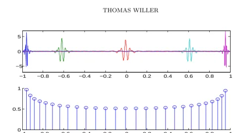
a(l/2j−1)Pl(η)pbj,η. Some examples of needlets are given on top of figure 5.3. Now we give a list of their properties needed to establish Theorem 2.
Wavelet-like properties: First of all, the needlets form a tight frame:
∀f∈H, f= X j∈Nη∈Zj hf, ψj,ηiψj,η and kfk2 = X j∈Nη∈Zj |hf, ψj,ηi|2.
Secondly each needletψj,ηk is concentrated on a small interval centered onη, as established in Petrushev and Xu (2005):
Theorem 4. For any l≥1 there exists a constant Cl> 0 such that
|ψj,ηk(cosθ)|≤Clp 1 ωα,β(2j,cosθ) 2j/2 (1+2j|θ− πk 2j|)l , 0≤θ≤π.
This almost exponential concentration property implies wavelet-like inequalities for the Lp norms of linear combinations of needlets. This is Theorem 5, estab-lished in Kerkyacharian, Picard, Petrushev, and Willer (2007):
Theorem 5. Let 0 < p <∞. Then there exists a constantCp> 0such that for any collection of numbers {λk:k=1, 2, . . . , 2j},j≥0,
k 2j X k=1 λkψj,ηkkp Lp(µ)≤Cp 2j X k=1 |λk|pkψj,ηkkp Lp(µ).
Differences with first generation wavelets: Needlets are not issued from a trans-lation/dilatation scheme, hence major differences with classical wavelets. Let us for example describe the needlets at a given resolution levelj. First they are not distributed uniformly on the interval, but around the ηks. Second they behave quite differently depending on their locationsηin the interval, which is reflected in Theorem 4 by the variations of the functionωα,β(2j, .). This is illustrated in
figure 5.3: for a given resolution j, ”edge” needlets have different shapes than ”middle” needlets, and theLp norms are not constant with respect to η (except arguably forp= 2). More precisely concerningLp norms, the following bounds have been established in Petrushev and Xu (2005) (for the upper bounds) and in Kerkyacharian, Picard, Petrushev, and Willer (2007) (for the lower bounds). They play an important role for the proofs of Theorem 1 and 2.
Theorem 6. ∀0 < p≤∞,∀j∈N,we have up to scalars depending only on p: ∀1≤k≤2j−1, kψj,ηkkp 2j(α+1) kα+1/2 !1−2/p , ∀2j−1 < k≤2j, kψj,ηkkp 2j(β+1) (1+ (2j−k))β+1/2 !1−2/p .
−1 −0.8 −0.6 −0.4 −0.2 0 0.2 0.4 0.6 0.8 1 −5 0 5 −1 −0.8 −0.6 −0.4 −0.2 0 0.2 0.4 0.6 0.8 1 0 0.5 1
Figure 5.3: For a given resolutionj: some of the needletsψj,ηk (above), and the values of all theL
3
norms (below) whenηkvaries
Moreover unlike first generation wavelets, needlets do not form an orthonor-mal basis, but only a redundant frame. This leads to some specific difficulties for the study of the lower bound of the minimax risk. So we needed to prove the two new following results.
First we need an upper bound for the scalar products between needlets. This is given by Lemma 1.
Lemma 1. We have:
1. ∀j, j0, k, l such that|j0−j|≥2, hψj,ηk, ψj0,η
li=0.
2. ∀ζ > 0,∃cζsuch that∀j, j0, k, lwith|j0−j|≤1: |hψj,ηk, ψj0,ηli|≤
cζ
(1+|k−2j−j0l|)ζ.
Secondly we need a lower bound for the Lp norm of linear combinations of needlets. Note that a result as general as the upper bound of Theorem 5 is impossible. Indeed, for instance with the non null coefficientspbj,ηk introduced
in the definition of the needlets, one can check that: P2kj=1pbj,ηkψj,ηk = 0. However we establish the following result for needlets with a large enough distance between the indexes of theη’s, in the case wherepis an even integer:
Theorem 7. Letp∈2N∗. Then there exists a constantcp> 0and an integernp
and k, l∈Ij, k6=l=⇒|k−l|≥np, kX k∈Ij λkψj,ηkk p Lp(µ)≥cp X k∈Ij |λk|pkψj,ηkk p Lp(µ).
Proof of Lemma 1. As indicated previously, the needlets are defined as: ψj,η =
P2j−1 l=2j−2+1cj,η,lPl(x),with coefficientscj,η,l=a(l/2j−1)Pl(η) p bj,η. So if|j0−j|≥ 2 then {2j−2 +1, . . . , 2j−1}∩{2j0−2+1, . . . , 2j0 −1} = ∅, and hψj,ηk, ψj0,η li = 0, ∀(k, l).
For the second part of the lemma we use Theorem 4. For any δthere exists
cδ such that for allj, k:
|ψj,ηk(cosθ)|≤cδp 1 ωα,β(2j,cosθ) 2j/2 (1+2j|θ− πk 2j|)δ , 0≤θ≤π.
We recall thatωα,β(x) = (1−x)α(1+x)β,andωα,β(2j;x) = (1−x+2−2j)α+1/2(1+
x+2−2j)β+1/2. For a given ζ > 0and j, j0, k, lsuch that |j0−j| ≤1, we use this inequality for |ψj,ηk| with δ = ζ+2 and for |ψj0,η
l| with δ = ζ. Noticing that
ωα,β(2j,cosθ)ωα,β(2j0,cosθ) we obtain:
|hψj,ηk, ψj0,η li|≤c2 j Zπ 0 ωα,β(cosθ) ωα,β(2j,cosθ) sinθdθ (1+2j|θ− πk 2j|)ζ+2(1+2j 0 |θ− πl 2j0|) ζ ≤c Ij,k,α,β (min0≤θ≤πfj,j0,k,l(θ))ζ , with fj,j0,k,l(θ) = (1+2j|θ− πk 2j|)(1+2j 0 |θ− πl 2j0|), 0 ≤ θ ≤ π, and Ij,k,α,β = 2jRπ 0 ωα,β(cosθ) ωα,β(2j,cosθ) sinθdθ (1+2j|θ−πk 2j|) 2.
First we have: min0≤θ≤πfj,j0,k,l(θ) = min{fj,j0,k,l(πk
2j), fj,j0,k,l(πl
2j0)} ≥ 1 +
π
2|j−j0||k−2j−j
0
Ij,k,α,β =I1 j,k,α,β+I2j,k,α,β, with: I1j,k,α,β =2j Zπ 2 0 ωα,β(cosθ) ωα,β(2j,cosθ) sinθdθ (1+2j|θ− πk 2j|)2 , I2j,k,α,β =2j Zπ π 2 ωα,β(cosθ) ωα,β(2j,cosθ) sinθdθ (1+2j|θ− πk 2j|)2 =2j Zπ 2 0 ωα,β(−cosθ) ωα,β(2j,−cosθ) sinθdθ (1+2j|π−θ− πk 2j|)2 =2j Zπ 2 0 ωβ,α(cosθ) ωβ,α(2j,cosθ) sinθdθ (1+2j|θ− π(2j−k) 2j |)2 =I1j,2j−k,β,α.
We have: sinθωα,β(cosθ) =sinθ(2sin2(θ/2))α(2cos2(θ/2))β≤c1θ2α+1, for all
0≤θ≤ π2, and:
ωα,β(2j;cosθ) = (2sin2(θ/2) +2−2j)α+1/2(2cos2(θ/2) +2−2j)β+1/2 ≥c2θ2α+1.
Thus I1j,k,α,β ≤ c2jR π 2 0 (1+2j|dθθ−πk 2j|) 2 ≤c Rπ2j 2 0 (1+|θdθ−πk|)2 ≤ C, since R+∞ −∞ dθ (1+θ)2 is
finite, and the same goes forI2 j,k,α,β.
Thus there exists C(α, β) > 0 such that for all (j, k): Ij,k,α,β ≤ C(α, β),
which completes the proof of the lemma.
Proof of Theorem 7. Let p∈ 2N∗ and Ij ⊂ {1, 2, . . . , 2j}. We have the following
decomposition: k(Pk∈I jλkψj,ηk)k p Lp(µ)=A+B, where: A= X k∈Ij λpkkψj,ηkkp Lp(µ), B= X (pk)k∈Ij∈Λ p!Qk∈I jλ pk k Q k∈Ijpk! Z1 −1 (Y k∈Ij ψpk j,ηk(x))µ(x)dx, and Λ = {(pk)k∈Ij | pk ∈ N, P
k∈Ijpk = pand ∃u 6= vsuch that pu >
Let us introduce the functionsϕj,k(x) = √ 1 ωα,β(2j,x) 2j/2 (1+2j|arccosx−πk 2j|) 2 s ,for some
0 < s <min{1,α∨pβ+1}.For (pk)k∈Ij ∈ Λ, we use Theorem 4 with l=
2
s +1 for
everyψj,ηk,k∈Ij. There exists Csuch that:
Y k∈Ij |ψj,ηk(cosθ)|pk ≤CY k∈Ij ϕj,k(cosθ)pk Y k∈Ij 1 (1+2j|θ− πk 2j|)pk .
Letu, v∈Ij, u6=vsuch thatpu> 0andpv > 0, and letninf=mink,l∈Ij,k6=l|k−
l|. We have: Y k∈Ij (1+2j|θ− πk 2j |) pk≥(1+2j|θ− πu 2j |)(1+2 j|θ−πv 2j|)≥c|u−v|≥cninf. Thus we obtain: X (pk)k∈Ij∈Λ p!Qk∈I j|λ pk k | Q k∈Ijpk! Y k∈Ij |ψj,ηk|pk ≤ C ninf X (pk)k∈Ij∈Λ p!Qk∈I j|λk| pk Q k∈Ijpk! Y k∈Ij ϕpk j,ηk ≤C (Pk∈I j|λk|ϕj,ηk) p ninf .
Now let us proceed similarly to the sketch of the proof of theorem 5 available in Kerkyacharian, Picard, Petrushev, and Willer (2007). Let us recall the two main tools.
First, consider the maximal operator(Msf)(x) =supJ3x
1 |J| R J|f(u)|sdu 1/s ,
where the supremum is taken over all intervalsJ⊂[−1, 1]which containx,s > 0, and |J| denotes the length of J. Then one can infer the following bound from the Fefferman-Stein maximal inequality (see Fefferman and Stein (1971)). If
0 < p, r <∞ and 0 < s < min{p, r,α∨pβ+1}, then for any sequence of functions (fk) on [−1, 1] X k (Msfk)r1/r Lp(µ)≤ C X k |fk|r1/r Lp(µ) .
Secondly set η0 = 1 and η2j+1 = −1, denote Ik = [ηk+η2k+1,ηk+η2k−1] and
put Hk = hk1Ik with hk = 2j
ωα,β(2j;ηk)
1/2
, where1Ik is the indicator function of Ik. ThenkHkkLp(µ) kψj,ηkkLp(µ), and one shows in Kerkyacharian, Picard, Petrushev, and Willer (2007) that for anys > 0
We use these two results, with fk = Hk and r= 1. Noticing that the (Hk) have disjoint supports, we obtain:
k 2j X k=1 |λk|ϕj,ηkkp Lp(µ) ≤Ck 2j X k=1 |λk|Hkkp Lp(µ)=C 2j X k=1 |λk|pkHkkp Lp(µ) ≤C0 2j X k=1 |λk|pkψj,ηkkp Lp(µ).
So finally there existsC > 0such that|B|≤CnA
inf,and if we impose the following
condition onIj: ninf≥2C, then we obtain|B|≤ 12A, and thus:
k(X k∈Ij λkψj,ηk)k p Lp(µ)≥ 1 2 X k∈Ij λpkkψj,ηkk p Lp(µ). Acknowledgment
The author would like to thank Professor Dominique Picard and the referees for their insightful comments on the paper.
References
Abramovich, F. and Silverman, B. W. (1998). Wavelet decomposition ap-proaches to statistical inverse problems. Biometrika 85(1):115-129.
Antoniadis, A. Fan, J. and Gijbels, I. (2001). A wavelet method for unfolding sphere size distributions. The Canadian Journal of Statistics 29:265-290. Cavalier, L. and Hengartner, N. W. (2005). Adaptive estimation for inverse
problems with noisy operators. Inverse problems 21, 1345-1361.
Cavalier, L. and Raimondo, M. (2007). Wavelet deconvolution with noisy eigen-values. IEEE Transactions on Signal Processing 55(6) part 1.
Cavalier, L. and Tsybakov, A. B. (2002). Sharp adaptation for inverse problems with random noise. Probab. Theory Related Fields 123(3):323-354.
Cavalier, L. Golubev, G. K. Picard, D. and Tsybakov, A. B. (2002). Oracle inequalities for inverse problems. Ann. Statist. 30(3):843-874.
Cruz-Orive, L. M. (1983) Distribution-free estimation of sphere size distribu-tions from slabs showing overprojecdistribu-tions and truncadistribu-tions, with a review of previous methods. J. Microscopy 131:265-290.
Donoho, D. L. (1995) Nonlinear solution of linear inverse problems by wavelet-vaguelette decomposition. Appl. Comput. Harmon. Anal. 2(2):101-126. Efromovich, S. and Koltchinskii, V. (2002). On inverse problems with unknown
operators. IEEE Trans. Inform. Theory 47(7):2876-2894.
Fan, J. and Koo, J. Y. (2002). Wavelet deconvolution. IEEE Trans. Inform. Theory 48 (3):734-747.
Fefferman, C. and Stein, E. M. (1971). Some maximal inequalities. Amer. J. Math. 93:107-115.
Goldenshluger, A. and Pereverzev, S. V. (2003). On adaptive inverse estimation of linear functionals in Hilbert scales. Bernoulli 9(5):783-807.
Golubev, G. K. and Levit, B. Y. (1998). Asymptotically efficient estimation in the Wicksell problem. Ann. Statist. 26(6):2407-2419.
H¨ardle, W. Kerkyacharian, G. Picard, D. and Tsybakov, A. B. Wavelets, Ap-proximation and Statistical Applications Springer-Verlag.
Hoffmann, M. and Reiss, M. (2007). Nonlinear estimation for linear inverse problems with error in the operator. Annals of Statistics (to appear). Johnstone, I. M. and Silverman, B. W. (1991). Discretization effects in
statis-tical inverse problems. J. Complexity 7(1):1-34.
Johnstone, I. M. Kerkyacharian, G. Picard, D. and Raimondo, M. (2004). Wavelet deconvolution in a periodic setting. Journal of the Royal Statistical Society 66(3):1-27.
Kalifa, J. and Mallat, S. (2003). Thresholding estimators for linear inverse problems and deconvolutions. Ann. Statist. 31(1):58-109.
Kerkyacharian, G. Picard, D. Petrushev, P. and Willer, T. (2007). Needlet algo-rithms for estimation in inverse problems. Electronic Journal of Statistics
Math´e, P. and Pereverzev, S. V. (2003). Geometry of linear ill-posed problems in variable Hilbert scales. Inverse Problems 19(3):789-803.
Narcowich, F. J. Petrushev, P. and Ward, J. M. (2006). Decomposition of besov and triebel-lizorkin spaces on the sphere. J. Funct. Anal. 238:530-564 Nychka, D. Wahba, G. Goldfarb, S. and Pugh, T. (1984). Cross validated spline
methods for the estimation of three-dimensional tumor size distributions from observations on two-dimensional cross sections. J. Amer. Statist. Assoc. 79:832-846.
Pensky, M. and Vidakovic, B. (1999). Adaptive wavelet estimator for nonpara-metric density deconvolution. Annals of Statistics 27:2033-2053.
Petrushev, P. and Xu, Y. (2005). Localized polynomial frames on the interval with Jacobi weights. J. Fourier Anal. Appl. 11(5):557-575.
Szeg¨o, G. (1975). Orthogonal polynomials. American Mathematical Society, Providence, R.I.
Tsybakov, A. B. (2000). On the best rate of adaptive estimation in some inverse problems. C. R. Acad. Sci. Paris S´er. I Math. 330(9):835-840.
Tsybakov, A. B. (2004). Introduction `a l’estimation non-param´etrique. Volume 41 of Math´ematiques and Applications, Springer-Verlag, Berlin.
Wicksell, S. D. (1925). The corpuscle problem: a mathematical study of a biometric problem. Biometrika 17:84-99.
Willer, T. (2005). Deconvolution in white noise with a random blurring effect.
preprint LPMA.
Willer, T. (2006). Non parametric estimation and inverse problems. Ph.D. thesis, Universit´e Paris 7.
Laboratoire d’Analyse, Topologie et Probabilit´es, Universit´e de Provence, Mar-seille, France