Block Bootstrap and Long Memory

Full text

(1)School of Economics and Finance Block Bootstrap and Long Memory. George Kapetanios and Fotis Papailias Working Paper No. 679. June 2011. ISSN 1473-0278.

(2) Block Bootstrap and Long Memory George Kapetanios School of Economics and Finance, Queen Mary University of London Fotis Papailias School of Economics and Finance, Queen Mary University of London June 3, 2011. Abstract We consider the issue of Block Bootstrap methods in processes that exhibit strong dependence. The main di¢ culty is to transform the series in such way that implementation of these techniques can provide an accurate approximation to the true distribution of the test statistic under consideration. The bootstrap algorithm we suggest consists of the following operations: given xt I (d0 ), 1) estimate the long memory b 2) di¤erence the series db times, 3) apply the block bootstrap on the above and parameter and obtain d, …nally, 4) cumulate the bootstrap sample db times. Repetition of steps 3 and 4 for a su¢ cient number. of times, results to a successful estimation of the distribution of the test statistic. Furthermore, we establish the asymptotic validity of this method. Its …nite-sample properties are investigated via Monte. Carlo experiments and the results indicate that it can be used as an alternative, and in most of the cases to be preferred than the Sieve AR bootstrap for fractional processes. JEL Code: C15; C22; C63. Keywords: Block Bootstrap; Long Memory; Resampling; Strong Dependence.. 1. Introduction. Since the seminal paper by Efron (1979), the bootstrap has increased rapidly in popularity. The two major factors that contributed to this are: (i) the decreased computational cost and, (ii) the improved theoretical results that stress that under mild conditions the bootstrap provides empirical approximations that are at least as accurate as the approximations implied by the …rstorder asymptotic distribution theory. In the nonparametric methodology of Efron (1979), the sampling distribution of iid observations is estimated by resampling. Carlstein (1986) and Kunsch (1989) introduced resampling techniques for weakly dependent stationary observations. In these, the data is divided in blocks which are approximately independent and the joint distribution of the variables in di¤erent blocks is about to be the same due to stationarity. In the …rst one, the blocks do not overlap one another (henceforth Corresponding Author. School of Economics and Finance, Queen Mary, University of London, Mile End Road, E1 4NS. E-mail Address: [email protected]. We are grateful to E. Guerre for insightful comments.. 1.

(3) denoted by N BB), whereas in the second method blocks are overlapping (henceforth mentioned as M BB). Politis and Romano (1992) and Politis and Romano (1994) introduced two other closely related methods: the Circular Block Bootstrap (henceforth denoted by CBB) and the Stationary Bootstrap (henceforth mentioned as SB). In both these methods the observed series are extended periodically and due to this common characteristic, their generalization is called the Dependent Bootstrap (see Politis and White (2004)). It is worth noticing here that the CBB and SB share the same asymptotic properties with the M BB, resulting however in better …nite sample estimates. A crucial issue to all the above techniques is the optimal choice of block length. Hall, Horowitz and Jing (1995) suggested that block length varies given speci…cations of di¤erent models. However, they concluded that three potential choices for the block length could be b = n ,. 2. 1 1 1 3; 4; 5. where. n denotes the sample size. Buhlmann and Kunsch (1999) introduced a data-dependent algorithm that results to the optimal block choice based on the equivalence of the block bootstrap variance to a lag weight estimator of the spectral density. Politis and White (2004) and Patton, Politis and White (2009) established a data-dependent method that successfully provides the optimal block length for the CBB and the SB methods. The di¤erence among the two bootstraps is that SB uses blocks of random length. In particular, the distribution of the block lengths in the latter method is the Geometric with mean being the optimal block length of CBB. Despite the fact that signi…cant research has been done concerning the bootstrap and fractionally integrated series, there is little work that addresses the application of bootstrap to long memory processes. Poskitt (2007) introduced the most used bootstrap in I (d0 ) data, the Sieve Bootstrap, which is an extension of previous research by Kreiss (1992). Another approach was done by Hidalgo (2003) who suggested a valid resampling scheme in the frequency domain. More details can be found in Park (2002), Kapetanios (2004), Andrews (2006), Kapetanios and Psaradakis (2006) etc. This paper aims to provide a new block bootstrap procedure that can be applied in long memory processes with consistency. Following Lahiri (2003) and Lahiri (2006), a direct application of any of the block methods described above fails. The general idea of this study is to transform the original data in a weak dependent data, obtain block bootstrap resamples from that data and then re-transform the resamples such that the original dependence is preserved (or "imitated"). At …rst, we semi parametrically estimate the long memory parameter, d0 , denoting the estimator b Hence, from this point of view our method is not non parametric. However, neither our by d.. competitor, the Sieve AR bootstrap, is non parametric. Then, we apply the di¤erence operator, (1. b. L)d , and we obtain a weak dependent data. We resample from this data and we cumulate. the resamples using (1. L). db. . Following Hall, Horowitz and Jing (1995) and Politis and White. (2004) we use the same methods for the calculation of block sizes. Generic asymptotic results, 2.

(4) independent of the exact block method or block size, can be found in the appendix. Furthermore, we conduct a simulation study using di¤erent models and sample sizes and we compare them to the Sieve Bootstrap. The outcome is that the out bootstrap algorithm provides better …nite results than the Sieve Bootstrap and hence, it should be preferred. The rest of the paper is divided as follows: section 2 introduces the long memory topic and the Block Bootstrap methods we use, section 3 presents the bootstrap algorithm we propose, section 4 discusses numerical evidence on the distribution of the Normalized Sample Mean and the Gaussian Semi Parametric Estimator and, section 5 summarizes the conclusions.. 2. Preliminaries. 2.1. Long Memory and Sieve Bootstrap. In general, a fractionally integrated process xt can be represented as, (1. L)d0 xt = ut ; t = 1; :::; n. (1). where L is the lag operator, d0 is the long memory parameter and ut s I (0). For jd0 j. 0:5 the. series is stationary and invertible, whereas for 0:5 < jd0 j < 1 the variance is not …nite but still has a cumulative impulse response function with …nite sum. The fractional di¤erencing operator is de…ned by the binomial expansion as, (1. d0. L). =. 1 X j=0. where. (j d0 ) =1 ( d0 ) (j + 1). d0 L +. d0 (d0 2. 1). L2 :::;. (2). ( ) denotes the gamma function. This expansion can be written as, (1. d0. L). =. 1 X. j. (d0 ) Lj :. (3). j=0. The most well-known, bootstrap procedure for such data is the sieve bootstrap by Kreiss (1992) and Buhlmann (1997). Following Poskitt (2007), the sieve bootstrap algorithm suggests to: 1. …t an AR (h), h < 1, model in the data, obtain the residuals and create the standardized residuals denoted by u bt .. 2. Then, create a new randomly resampled series of the above, denoted by u bt . Apply the desired test statistic on a bootstrap resample xt that is generated by h AR terms and u bt error. 3.

(5) 3. By repeating the above procedure a number of times B we obtain a bootstrap approximation to the distribution of the test statistic. The order autoregressive order h can be derived using any information criterion, such as Akaike’s or Bayesian. Ng and Perron (1995) prove that under similar setup, AIC and BIC are asymptotically consistent.. 2.2. Block Bootstrap. The bootstrap succeeds in the approximation of the underlying distribution due to the assumption that observations are independent. The idea behind block bootstrap is similar. Blocks of observations of stationary processes should be approximately independent and due to stationarity the joint distribution of the variables in di¤erent blocks should be almost the same. The main di¢ culty we confront is the choice of that optimal block size that the above happens. Using data driven methods, like Hall, Horowitz and Jing (1995) and Politis and White (2004), we can …nd these choices. Suppose we have xt. I (0), t = 1; 2; :::; n, a choice of optimal block size, say b, and M =. n b. where. [ ] denotes integer part. Then, 1. xt : (a) (N BB) is divided in M disjoint blocks, the k 1. k. 1)b+1 ; :::; xkb. for. M,. (b) (M BB) is divided in (n for 1. th being xkN BB = x(k. k. (n. b)+1 overlapping blocks, the k th being xkM BB = xk ; :::; x(k+b). 1. b) + 1,. (c) (CBB) is wrapped around the beginning (periodically extended) as x1 ; x2 ; :::; xn ; x1 ; x2 ; :::; xn ; ::: . Then blocks are de…ned as xkCBB = fxk ; :::; xn+k. 1g :. (d) (SB) is wrapped around as before and the blocks de…ned are of random length. The distribution of the blocks, Fb , is the Geometric with mean equal to b. 2. Given our preferred block method described above, we randomly choose M blocks by resampling with replacement and we obtain xt = fx1 ; x2 ; :::; xM g. Then the test statistic is performed on this bootstrap data. 3. We repeat step 3 a number of times B, in order to obtain a bootstrap approximation to the distribution of the test statistic. As B ! 1 accuracy of results is guaranteed.. 4.

(6) 3. A Block Bootstrap Procedure for Long Memory Time Series. The key problem for the application of the Block Bootstrap in long memory time series is the degree of integration. In this part of the paper we propose a methodology that overcomes this di¢ culty. Given that the exact value of the degree of long memory is unknown, the main idea is to di¤erence the data using an estimate db in order to obtain weak dependence. Then, we cumulate. bootstrap resample db times using the estimate. Any method for the estimation of d that satis…es the following general assumption can be used. Assumption 1 db. d0 = Op n. ,. > 0.. d0 denotes the true degree of integration and n is the sample size The above is a rather general assumption that does not specify any particular method for. estimating d0 . It assumes consistency and some rate of convergence for the estimator. Note that there is complete literature regarding estimators with desirable asymptotic properties even when jd0 j > 0:5 (see Velasco (1999) etc.). However, this assumption does not allow for estimators whose rate of convergence depends on d0 . The algorithm we suggest consists of the following operations: 1. Given xt. I (d0 ), t = 1; 2; :::; n, we estimate the fractional exponent and we obtain db ; for. more details see Robinson (1995), Baillie and Kapetanios (2008) etc. 2. We di¤erence xt db times denoting the new series by zt , zt. I db. d0 .. 3. Using any of the block bootstrap methods described in the previous section, we create a b We denote the resulting series by bootstrap resample of zt and we cumulate it using d. zt. (d0 ). Then, the desired test statistic is applied.. 4. We repeat step 3 B times and we obtain a bootstrap approximation to the distribution of the test statistic. Theorem 1 Let distributions FX. (FX ; FY ) denote the Mallow’s measure of the distance between two probability n o1 2 and FY , de…ned as inf E kX Y k2 , where the in…mum is taken over all square. integrable random variables X and Y in R with marginal distributions FX and FY . Then, F. b db) ; FSn (d; Sn. = 0 as n ! 1,. where Sn denotes the test statistic, FSn denotes its true distribution and F bootstrap approximation. 5. b db) (d; Sn. denotes the.

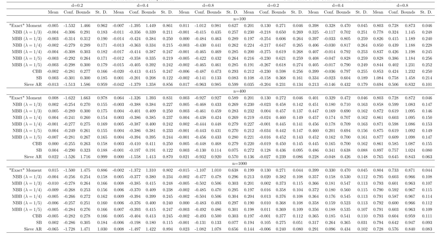
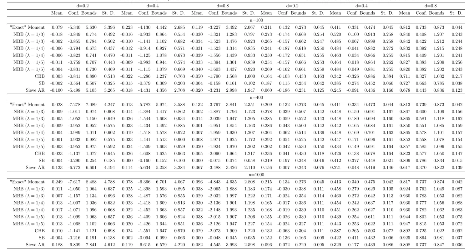
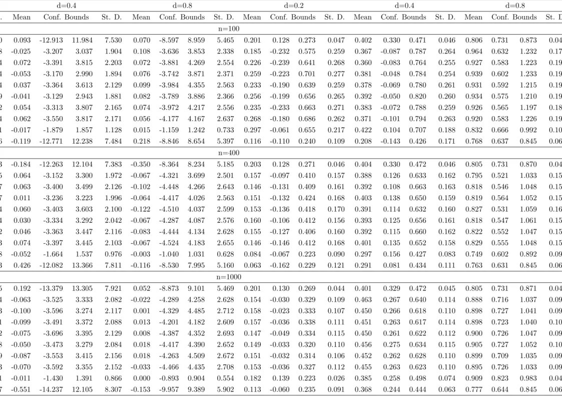
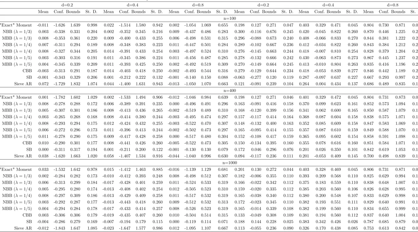
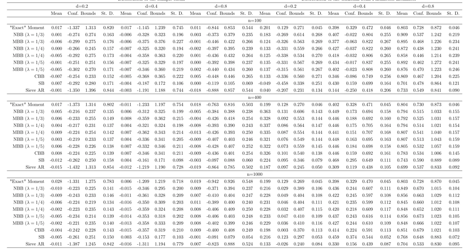
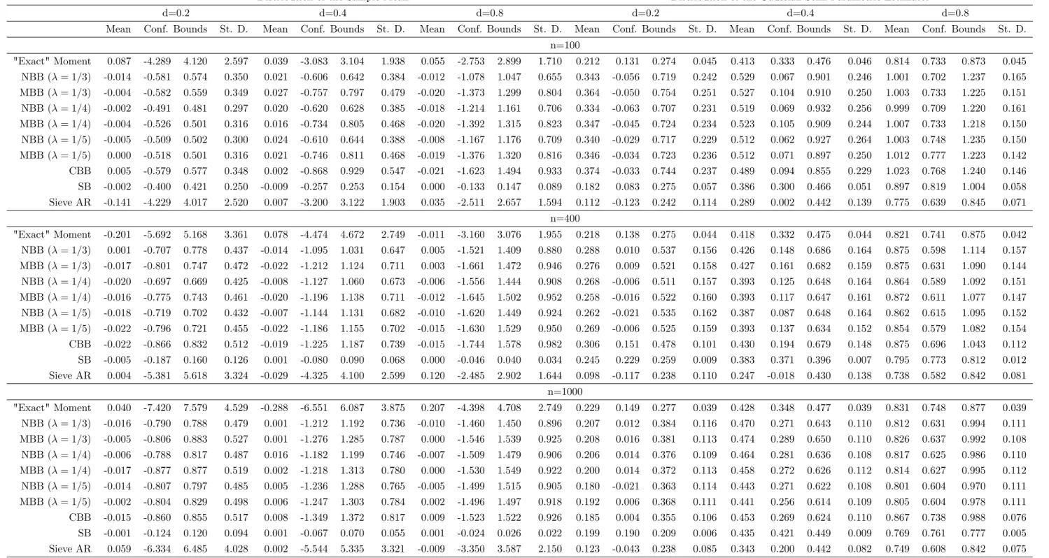
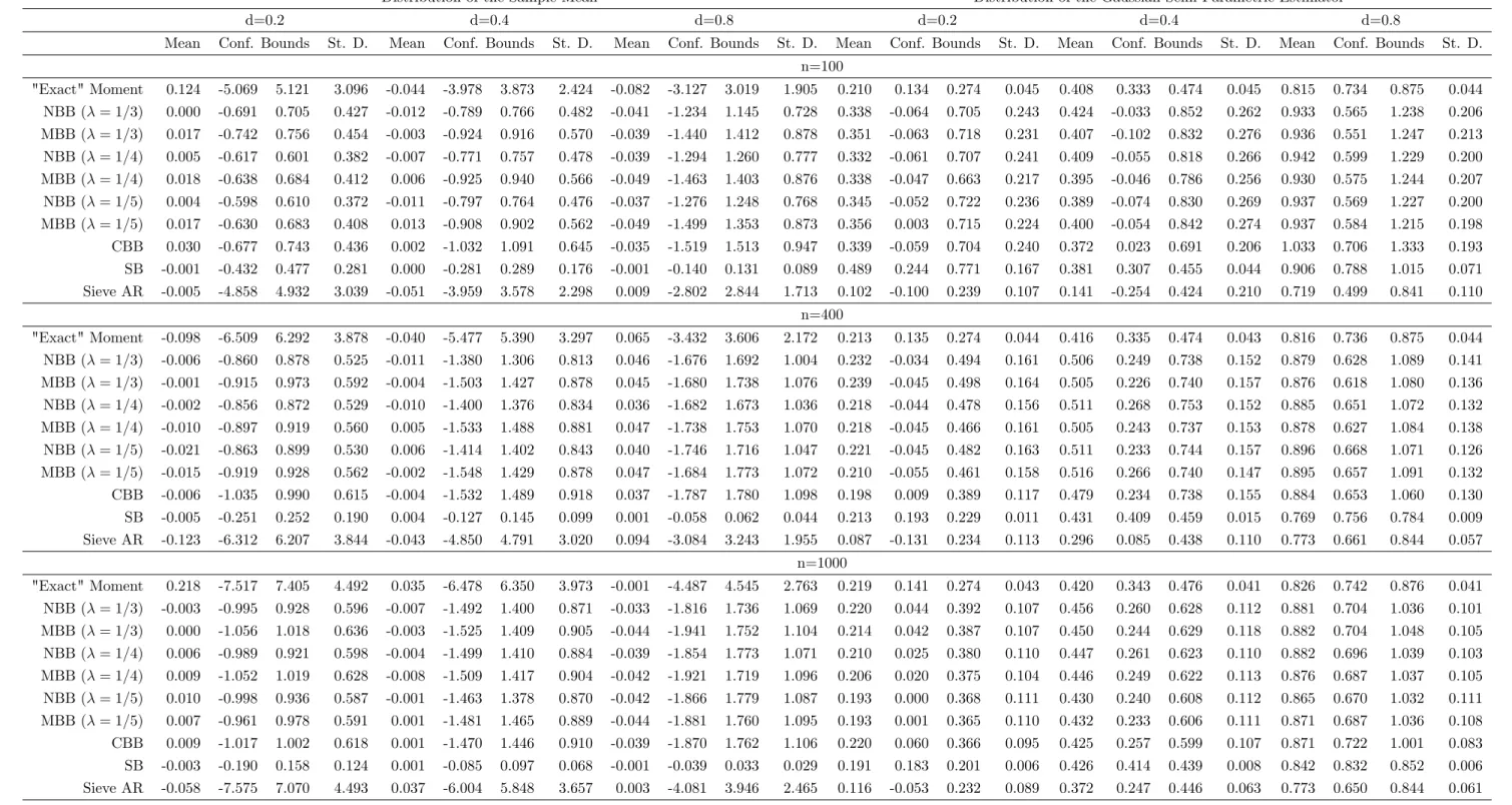
(7) The above theorem is closely related to Theorem 2 in Poskitt (2007) and states that the bootstrap estimate to the true distribution of the test statistic obtained using the previously described algorithm is consistent with the true distribution.. 4. Simulation Experiments. This section is concerned with numerical evidence that illustrates the …nite-sample performance of the block bootstrap for long range dependent processes. We discuss two sets of experiments, one for the case of the approximation to the distribution of the sample mean and one for the approximation to the distribution of the Gaussian Semi Parametric Estimator, commonly referred to as the Local Whittle. In all experiments we use ARF IM A (p; d; q) models to generate the data. Speci…cally, we present the following designs: ('1 ; #1 ) = (0; 0), ('1 ; #1 ) = (0:8; 0), ('1 ; #1 ) = (0; 0:8), ('1 ; #1 ) = ( 0:3; 0:4), ('1 ; #1 ) = (0:3; 0:4), ('1 ; '2 ; #1 ) = (0:2; 0:7; 0) and ('1 ; '2 ; #1 ) = (0:7; 0:2; 0). For each case the error term is standard normal, d 2 f0:2; 0:4; 0:8g and the sample size is n 2 f100; 400; 1000g. Tables 1 - 7 present the mean and variance of the estimate of the true distribution of the sample mean and Gaussian Semi Parametric Estimator along with the 95% con…dence intervals for the mean. The db used in step 1 of the algorithm is obtained using the Gaussian Semi Parametric Estimator and. h = (ln n)2 for the sieve. The block sizes we use are those suggested by Hall, Horowitz and Jing (1995) and for the CBB and SB those introduced by Politis and White (2004).. 4.1. Normalized Sample Mean. The Exact Moments of the distribution of the sample mean are computed from 1000 Monte Carlo 1. values of n 2. d0. (xn. ), where. = 0. Similarly, the bootstrap estimates are computed as averages 1. of 1000 Monte Carlo trials of 199 bootstrap resamples of n 2 of the bootstrap algorithm in section 3.. db. zn. xn , in respect to the notation. The simulation results suggest that the block bootstrap approximates very well the distribution of the sample mean. Especially when the block method is the CBB or SB; in most of the experiments in large samples (n > 400), the results are better than those provided by the Sieve AR. This is a very promising result given that it argues and questions why we have to favor the Sieve AR bootstrap in practice, especially when it provides highest mean square error of the moment estimates than any of block bootstrap methods.. 6.

(8) 4.2. Gaussian Semi Parametric Estimator. It has been a great debate in the literature about the estimation methods of long range dependent time series. A common argument in favor of the semi parametric setup is that speci…cation di¢ culties of the short-run components can be avoided. Geweke and Porter - Hudak (1983) introduced one of the early semi parametric methods in the frequency domain. However Agiakloglou, Newbold and Wohar (1992) showed its poor performance in relation to the short run dynamics. In more recent years, the Gaussian Semi Parametric Estimator of long range dependence, or Local Whittle, of Robinson (1995) is the most preferred method due to its satisfying statistical properties. Extensions of the above in nonlinear and non stationary time series have been developed by Dalla, Giraitis and Hidalgo (2005) and Velasco (1999) respectively. b is obtained minimizing the following objective The Local Whittle estimator of d0 , denoted by d,. function,. 2. 3 m X 1 0 5 ! 2d R (d0 ) = log 4 j I (! j ) m. m. 1 X log ! j , 2d0 m. j=1. (4). j=1. where I (! j ) is the periodogram of the series in the ! j Fourier frequencies, j = 1; 2; :::; m where m < n2 . Generally, m is chosen so that. 1 m. +m n ! 0 as n ! 1. Obviously, the estimator is sensitive. on that matter. Henry (2001) provides data dependent method for the choice of m.. Following. Robinson (1995), 1 m 2 db. d0 !d N. 0;. 1 4. ,. (5). where d0 denotes the true value. Generally, in the ignorance of short run dynamics, m is chosen to be m = n1=2 and this is also the choice in our experiments. The Exact Moments of the distribution of the Local Whittle are computed from a 1000 Monte Carlo replications, and the bootstrap estimates are computed from averages of 1000 bootstrap resamples as in step 3 of the bootstrap algorithm. In the vast majority of the experiments the same result as in the case of normalized sample mean is repeated. The CBB and SB provide better estimates for the moments of the distribution of the Local Whittle making the Sieve to be the next best option. Particularly, the Sieve Bootstrap performs better in the vanilla ARF IM A (0; d; 0) model. In more complex cases like ARF IM A (1; d; 0) and ARF IM A (2; d; 0) for all values of d0 and in all sample sizes, the SB dominates. At this point it can be argued that our method heavily relies on the estimation of the long memory parameter and also, from this point of view, our method is semi parametric. This is true. The use of a biased estimate of d0 when applying the di¤erencing operator might result in a "not so weak" dependent data (zt in step 2 of our algorithm), especially when the true long memory. 7.

(9) parameter is high (e.g. d0 = 0:9 and db = 0:2). However, this phenomenon is extremely rare. in the most common data that is being used in practice. Regarding the setup of our bootstrap. methodology, nonparametric econometrics are indeed much favored to semi or full parametric. However, given the nature of the problem, which is the unknown degree of integration, the initial estimation of d cannot be avoided. Furthermore, one must have in mind that neither the Sieve AR Bootstrap is non parametric.. 5. Conclusion. In this paper we introduce the block bootstrap in strongly dependent time series. To the best of the authors’ knowledge, application of block bootstrap in long memory time series has not been researched before. In practice, the Sieve AR bootstrap is the most commonly used. Our algorithm tries to avoid the complicated steps of Sieve (i.e. at …rst the AR (P ) order must be obtained and secondly the model has to be estimated in order to retrieve the residuals). The procedure we suggest is described in the following steps: we di¤erence the data using a valid estimate of the long memory parameter, we apply the block bootstrap of our choice and we cumulate this bootstrap resample using the same estimate. Repetition of the above procedure guarantees accurate approximation to the distribution of the test statistic. The greatest advantage of the block bootstrap is the ease-of-use, making the applied researcher’s work less complicated. At her favor, the numerical experiments provide evidence that our method estimates very well the distribution of the sample mean and the Gaussian Semi Parametric Estimator and can provide more accurate approximations in …nite samples especially when the SB is used. To conclude with, this paper shows adequate evidence that, at last, the Block Bootstrap can be applied in fractionally integrated processes successfully.. 6. Appendix. In this appendix we go through the asymptotic results of the bootstrap procedure described in section 3. Before we proceed with the proof of theorem 1, we …rst de…ne some additional theory and notation. Using each step of the algorithm and the original long memory series xt have already de…ned zt. I (d0 ), we. I (d0 ) as the bootstrap resample using db in di¤erencing and cumulating. (steps 2 and 3 respectively).. In addition to that, we also de…ne yt. I (d0 ) as the bootstrap resample in the theoretical. case where d0 is known and is used for di¤erencing and cumulation and, ht 8. I db. 2d0. as the.

(10) bootstrap resample in the case where we use db for di¤erencing and d0 for cumulation.. The relevant bootstrap approximations to the true distribution of the test statistic are denoted. by F. b db) , (d; Sn. FS. (d0 ;d0 ) n. and F. b (d;d 0) Sn. respective to zt , yt and ht .. Following Poskitt (2007), we make use of the following assumption (assumption 4 in his paper).. Assumption 2 Given a process xt and Xn = fx1 ; x2 ; :::; xn g, and the corresponding block bootstrap sample to be denoted by zt and hence, Zn = fz1 ; z2 ; :::; zn g, let N be a compact subset of Rn . Then for all Xn ; Zn N there exists a family of Borel measurable functions Bt : Rn. Rn ! [0; 1),. satisfying,. lim sup. n!1. n ii 1X h h E E Bt (Xn ; Zn )2 < 1; n t=1. for which Sn. 2. b db) (d; Sn. n. 1X Bt (Xn ; Zn )2 jxt n t=1. zt j :. where, E [ ] is the expectation taken with respect to Pfx1 ;x2 ;:::;xn g , E [ ] is the expectation taken with respect to Pfz ;z ;:::;z g , Sn and Sn are the test statistics using the original and bootstrap samples n 1 2 respectively. Proof. Then we have that, 2. F. b db) (d;. Sn. ; F Sn. 2. F F. b db) (d;. Sn. b db) (d;. Sn. ; FS. +. (d0 ;d0 ) n. 2. ;F. b (d;d. Sn. +. 0). n. FS F. (d0 ;d0 ) ; FSn. n. b (d;d. Sn. ; FS 0). o2. (d0 ;d0 ) n. 2. +. n. FS. (d0 ;d0 ) ; FSn. n. (6). The last term of the right hand side of the above is straightforward because d0 is used, see Kunsch (1989) and Politis and White (2004). Thus, we focus our interest on the …rst and second terms. From the de…nition of Mallow’s metric, using assumption 2 and applying the Cauchy-Schwartz. 9. o2.

(11) inequality twice we have, ". 2. F. b db) ; F b (d; (d;d 0) Sn Sn. ". E E. b db) (d;. Sn. Sn. n n ii 1 X h h 1X h h 2 E E (Bn (Hn ; Zn )) E E (ht n n t=1. 2. b 0) (d;d. ##. zt )2. t=1. n n ii 1 X h h 1X h h 2 E E (Bn (Hn ; Zn )) E E (ht lim sup n!1 n n t=1. ii zt )2. t=1. n ii 1X h h = lim sup E E (Bn (Hn ; Zn ))2 n!1 n. n 1X h h lim sup E E (ht n!1 n. t=1. ii. zt )2. t=1. ii. :. (7). Given that there exists such function Bn (Hn ; Zn ) so that the …rst sup limit is …nite, we are interested in the last term of the right hand side of the above. Hence, we need to prove that, lim sup. n!1. n 1X h h E E (ht n. zt )2. t=1. ii. = 0:. (8). By the de…nition of the long memory processes in eq. (1) we have that, b d0. L)d. ht = (1. zt :. (9). Following the same analysis with Wright (1995) and using eq. (3), ht. zt. =. t 1 X. db. j. j=1. db. = since, j. where. 0 j. and. 00 j. db. d 0 zt. t 1 X. d0. db. 0 j. j=1. d0 = db. j. d0. d 0 zt. 0 j. db. j. + db. d0. j. eq. (8) and eq. (10), we need to prove that, 2 20 n X 1 E 4E 4@ db lim sup n!1 n t=1. d0. t 1 X j=1. 0 j. db. d 0 zt. This follows from the fact that the variance of db lim sup E E. n!1. 10. j. db. 00 j. j=1. d0 + db. denote the …rst and second derivative of. t 1 2X. + db. d0. 2. 00 j. db. d 0 zt. j. ,. (10). d0 ;. (11). respectively for db. d0 ! 0. Using. d0. t 1 2X j=1. 00 j. db. d 0 zt. j. 12 33. A 55 = 0:. (12). d0 goes to zero when n ! 1, db. d0. 2. = 0:. (13).

(12) Indeed, the …rst limit of the identity of eq. (12) can be written as, 2 20 n 1 X 4 4@ b E E d lim sup n!1 n. t 1 X. d0. t=1. db. lim sup E E. n!1. j=1. d 0 zt. 2 20 n t 1 X X 1 lim sup E 4E 4@ n!1 n. 2. d0. db. 0 j. t=1. 0 j. j=1. j. 12 33 A 55. db. d 0 zt. j. 12 33. A 55 ;. (14). where the second limit is …nite. Following the limit theorem by Robinson (1995) in eq. (5) and eq. (14, 13), eq. (12) is proved. Similarly, ". 2. F. ; FS (d0 ;d0 ) b (d;d 0) n Sn. E E. ". 2. b 0) (d;d. Sn(d0 ;d0 ). Sn. ##. n n ii 1 X h h 1X h h 2 E E (Bn (Yn ; Hn )) E E (yt n n t=1. ht )2. t=1. n n ii 1 X h h 1X h h 2 lim sup E E (Bn (Yn ; Hn )) E E (yt n!1 n n t=1. ii ht )2. t=1. n ii 1X h h lim sup E E (Bn (Yn ; Hn ))2 n!1 n. ii. n 1X h h lim sup E E (yt n!1 n. t=1. ht )2. t=1. ii. ;. and hence we need to prove that, n 1X h h lim sup E E (yt n!1 n. ht )2. t=1. ii. = 0:. (15). As before we have that, b d0. L)d. ht = (1. yt :. (16). Now,. yt. ht. =. =. (ht 0. @ db. 0 t 1 X @. yt ) =. j. j=1. d0. t 1 X. 0 j. j=1. db. db. d 0 yt. d 0 yt. j. j. 1 A. + db. d0. t 1 2X. 00 j. j=1. db. d 0 yt. j. 1. A:. (17). We need to prove that, 2 20 0 n X 1 lim sup E 4E 4@ @ db n!1 n t=1. d0. t 1 X j=1. 0 j. db. and as before, the result follows.. 11. d 0 yt. j. + db. d0. t 1 2X j=1. 00 j. db. d 0 yt. j. 112 33. AA 55 = 0 (18).

(13) References AGIAKLOGLOU, C., NEWBOLD, P., and M., WOHAR (1992) Bias in an Estimator of the Fractional Di¤erencing Parameter, Journal of Time Series Analysis, 14, 235-246. ANDREWS, D. W. K., and O., LIEBERMAN (2006) Higher-order Improvements of the Parametric Bootstrap for Long-memory Gaussian Processes, Journal of Econometrics, 133, 673-702. BAILLIE, R. T., and G., KAPETANIOS (2008) Semiparametric Estimation of Long Memory Models: Comparisons and some attractive Alternatives, Working Paper, Michigan State University, Working Papers. BUHLMANN, P. (1997) Sieve Bootstrap for Time Series, Bernoulli, 3, 2, 123-148. BUHLMANN, P., and H., R., Kunsch (1999) Block Length Selection in the Bootstrap for Time Series, Computational Statistics and Data Analysis, 31, 295-310. DALLA, V., GIRAITIS, L. and J., HIDALGO (2005) Consistent Estimation of the Long Memory Parameter for Nonlinear Time Series, Journal of Time Series Analysis, 27, 211-251. DasGupta, A. (2008) Asymptotic Theory of Statistics and Probability, Springer. CARLSTEIN, E. (1986) The Use of Subseries Values for Estimating the Variance of a General Statistic from a Stationary Sequence, Annals of Statistics, 14, 1171-1179.. EFRON, B. (1979) Bootstrap Methods: Another Look at the Jackknife, Annals of Statistics,7, 1-26. GEWEKE, J., and S., PORTER-HUDAK (1983) The Estimation and Application of Long Memory Time Series Models, Journal of Time Series Analysis, 4, 221-238. HALL, P., HOROWITZ, J. L. and B.Y., JING (1995) On Blocking Rules for the Bootstrap with Dependent Data, Biometrika, 82, 561-574. HENRY, M. (2001) Robust Automatic Bandwidth for Long Memory, Journal of Time Series Analysis, 22, 292-316. HENRY, M., and P. M., ROBINSON (1996) Bandwidth Choice in Gaussian Semi Parametric Estimation of Long Range Dependence, in Athens Conference on Applied Probability and Time Series, Vol II: Time Series in Memory of E. J. Hannan, ed. by P. M. Robinson and M. Rosenblatt, Springer-Verlag.. 12.

(14) HIDALGO, J. (2003) An Alternative Bootstrap to Moving Blocks for Time Series Regression Models, Journal of Econometrics, 117, 369-399. HOROWITZ, J. L. (1999) The Bootstrap, In: Handbook in Econometrics, Elsevier, Heckman, J. J., Leamer, E., (Eds.). LAHIRI, S. N. (2003) Resampling Methods for Dependent Data, Springer-Verlag: New York. LAHIRI, S. N. (2006) Bootstrap Methods: A Review, In: Frontiers in Statistics, Imperial College Print, Fan, J., and H., Koul (Eds.). KAPETANIOS, G. (2004) A Bootstrap Invariance Principle for Highly Nonstationary Long Memory Processes, Working Paper No. 507, Queen Mary, University of London, Working Papers. KAPETANIOS, G. (2009) Testing for Strict Stationarity in Financial Variables, Journal of Banking and Finance, 33-12, 2346-2362. KAPETANIOS, G. and Z., PSARADAKIS (2006) Sieve Bootstrap for Strongly Dependent Stationary Processes, Working Paper No. 552, Queen Mary, University of London, Working Papers. KREISS, J. (1992) Bootstrap Procedures for AR (1) Processes, Springer: Heidelberg. KUNSCH, H.-R. (1989) The Jackknife and the Bootstrap for General Stationary Observations, Annals of Statistics, 7, 1-26. NG, S. and P., PERRON (1995) Unit Root Tests in ARMA models with data-dependent methods for the selection of the truncation lag, Journal of the American Statistical Association, 90, 268281. PATTON, A., POLITIS, D. N. and H., WHITE (2009) Correction to Automatic Block-Length Selection for the Dependent Bootstrap, Econometric Reviews, 28-4, 372-375. PARK, J. Y. (2002) An Invariance Principle for Sieve Bootstrap in Time Series, Econometric Theory, 18, 469-490. POLITIS, D. N. and J. P., ROMANO (1992) A Circular Block Resampling Procedure for Stationary Data, Exploring the Limits of Bootstrap, 263-270, Wiley - New York. POLITIS, D. N. and J. P., ROMANO (1994) The Stationary Bootstrap, Journal of American Statistical Association, 89, 1303-1313. POLITIS, D. N., ROMANO, J.P. and M., WOLF (1999) Subsampling, Springer: New York.. 13.

(15) POLITIS, D. N. and H., WHITE (2003) Automatic Block-Length Selection for the Dependent Bootstrap, Econometric Reviews, 23-1, 53-70. POSKITT, D. S. (2007) Properties of the Sieve Bootstrap for Fractionally Integrated and NonInvertible Processes, Journal of Time Series Analysis, 29, 2, 224-250. ROBINSON, P. M. (1995) Gaussian Semi-parametric Estimation of Long Range Dependence, Annals of Statistics, 23 (5), 1630–1661. VELASCO, C. (1999) Gaussian Semiparametric Estimation of Non-Stationary Time Series, Journal of Time Series Analysis, 20-1, 87-127. WRIGHT, J. H. (1995) Stochastic Orders of Magnitude Associated with Two-Stage Estimators of Fractional Arima Systems, Journal of Time Series Analysis, 16-1, 119-126. 14.

(16) Table 1. ARFIMA (0, d, 0) Distribution of the Sample Mean d=0.2 Mean. Conf. Bounds. -0.005 -0.004 -0.003 -0.002 -0.004 -0.003 -0.003 -0.002 0.003 -0.013. -1.532 -0.306 -0.314 -0.279 -0.308 -0.292 -0.298 -0.281 -0.301 -1.513. Distribution of the Gaussian Semi Parametric Estimator. d=0.4 St. D.. Mean. Conf. Bounds. 0.962 0.183 0.190 0.171 0.182 0.171 0.179 0.166 0.185 0.959. -0.007 -0.011 -0.014 -0.013 -0.017 -0.012 -0.015 -0.020 0.001 -0.042. -1.395 -0.356 -0.424 -0.363 -0.414 -0.358 -0.405 -0.413 -0.201 -1.379. d=0.8 St. D.. Mean. Conf. Bounds. 0.861 0.211 0.250 0.215 0.247 0.219 0.242 0.247 0.122 0.856. 0.011 -0.001 0.000 -0.003 -0.001 -0.005 -0.002 -0.006 -0.002 0.017. -1.012 -0.415 -0.484 -0.430 -0.465 -0.422 -0.465 -0.487 -0.141 -0.963. d=0.2 St. D.. Mean. Conf. Bounds. d=0.4 St. D.. Mean. Conf. Bounds. d=0.8 St. D.. Mean. Conf. Bounds. St. D.. n=100 "Exact" Moment NBB ( = 1=3) MBB ( = 1=3) NBB ( = 1=4) MBB ( = 1=4) NBB ( = 1=5) MBB ( = 1=5) CBB SB Sieve AR. 1.466 0.291 0.312 0.289 0.303 0.264 0.300 0.277 0.300 1.586. 1.449 0.339 0.384 0.334 0.387 0.335 0.392 0.415 0.208 1.358. 0.981 0.435 0.463 0.441 0.469 0.432 0.461 0.473 0.133 0.985. 0.627 0.257 0.289 0.262 0.285 0.264 0.285 0.293 0.083 0.599. 0.201 0.230 0.197 0.224 0.200 0.216 0.191 0.212 0.108 0.035. 0.130 -0.218 -0.254 -0.217 -0.275 -0.230 -0.267 -0.230 -0.158 -0.204. 0.271 0.650 0.606 0.647 0.619 0.621 0.618 0.598 0.368 0.231. 0.046 0.269 0.264 0.265 0.268 0.259 0.274 0.256 0.161 0.134. 0.398 0.325 0.397 0.406 0.407 0.408 0.405 0.399 0.334 0.213. 0.328 -0.117 -0.033 -0.030 -0.014 -0.047 -0.017 -0.036 -0.023 -0.146. 0.470 0.702 0.805 0.817 0.792 0.828 0.790 0.797 0.604 0.432. 0.045 0.251 0.259 0.264 0.253 0.259 0.249 0.255 0.189 0.179. 0.803 0.778 0.826 0.850 0.837 0.828 0.844 0.853 1.084 0.694. 0.728 0.324 0.415 0.439 0.426 0.386 0.402 0.424 0.758 0.506. 0.873 1.145 1.189 1.188 1.198 1.184 1.231 1.232 1.458 0.832. 0.046 0.248 0.240 0.228 0.245 0.256 0.252 0.250 0.214 0.101. 0.130 -0.023 0.004 -0.024 -0.001 -0.034 -0.016 -0.019 0.128 -0.027. 0.272 0.458 0.457 0.460 0.445 0.442 0.452 0.450 0.436 0.239. 0.046 0.142 0.137 0.149 0.141 0.147 0.143 0.145 0.095 0.086. 0.401 0.451 0.447 0.457 0.456 0.460 0.452 0.445 0.486 0.228. 0.329 0.180 0.169 0.174 0.178 0.201 0.162 0.165 0.341 -0.048. 0.472 0.710 0.690 0.707 0.709 0.694 0.700 0.700 0.638 0.426. 0.046 0.163 0.162 0.162 0.163 0.156 0.161 0.162 0.088 0.148. 0.803 0.858 0.872 0.861 0.871 0.875 0.877 0.861 0.897 0.765. 0.728 0.599 0.619 0.603 0.598 0.619 0.609 0.585 0.757 0.645. 0.872 1.083 1.095 1.095 1.086 1.092 1.098 1.087 1.024 0.843. 0.046 0.147 0.146 0.150 0.153 0.149 0.147 0.155 0.080 0.063. 0.130 0.020 0.002 0.016 0.013 0.010 0.011 -0.001 0.105 -0.006. 0.271 0.382 0.373 0.358 0.376 0.368 0.369 0.377 0.275 0.240. 0.044 0.108 0.115 0.104 0.108 0.108 0.109 0.112 0.051 0.080. 0.399 0.357 0.366 0.372 0.364 0.358 0.356 0.365 0.317 0.291. 0.330 0.158 0.181 0.180 0.176 0.159 0.188 0.185 0.264 0.096. 0.470 0.530 0.547 0.560 0.545 0.523 0.535 0.541 0.365 0.434. 0.045 0.112 0.113 0.115 0.113 0.113 0.107 0.110 0.031 0.102. 0.804 0.795 0.793 0.790 0.791 0.792 0.791 0.793 0.794 0.728. 0.733 0.603 0.601 0.592 0.587 0.600 0.603 0.604 0.642 0.576. 0.871 0.966 0.963 0.967 0.967 0.966 0.963 0.959 0.947 0.840. 0.044 0.108 0.107 0.115 0.114 0.112 0.109 0.111 0.093 0.083. n=400 "Exact" Moment NBB ( = 1=3) MBB ( = 1=3) NBB ( = 1=4) MBB ( = 1=4) NBB ( = 1=5) MBB ( = 1=5) CBB SB Sieve AR. 0.008 0.002 0.005 0.004 -0.001 0.004 -0.007 0.000 0.004 0.022. -1.622 -0.254 -0.289 -0.241 -0.277 -0.249 -0.281 -0.255 -0.290 -1.526. 1.663 0.270 0.300 0.260 0.275 0.261 0.267 0.263 0.323 1.716. 0.978 0.155 0.175 0.154 0.169 0.155 0.165 0.158 0.188 0.999. 0.064 -0.003 0.004 0.003 0.005 0.004 0.004 0.003 -0.001 0.000. -1.326 -0.388 -0.401 -0.386 -0.387 -0.386 -0.394 -0.410 -0.197 -1.558. 1.393 0.384 0.409 0.385 0.400 0.381 0.395 0.411 0.191 1.413. 0.831 0.227 0.250 0.237 0.242 0.233 0.244 0.250 0.122 0.870. 0.003 0.005 0.003 0.004 0.002 -0.001 -0.001 0.005 0.003 0.021. -0.927 -0.468 -0.461 -0.438 -0.444 -0.443 -0.456 -0.448 -0.130 -0.932. 0.927 0.433 0.459 0.424 0.448 0.431 0.433 0.468 0.114 0.920. 0.589 0.269 0.283 0.269 0.279 0.270 0.280 0.279 0.075 0.570. 0.201 0.230 0.232 0.219 0.227 0.212 0.221 0.220 0.272 0.136. n=1000 "Exact" Moment NBB ( = 1=3) MBB ( = 1=3) NBB ( = 1=4) MBB ( = 1=4) NBB ( = 1=5) MBB ( = 1=5) CBB SB Sieve AR. 0.015 -0.004 -0.010 -0.009 -0.005 -0.006 -0.005 -0.005 0.002 -0.065. -1.500 -0.256 -0.278 -0.268 -0.266 -0.257 -0.284 -0.282 -0.286 -1.728. 1.475 0.254 0.264 0.253 0.272 0.251 0.276 0.278 0.305 1.471. 0.886 0.158 0.166 0.156 0.162 0.160 0.166 0.166 0.184 1.030. -0.002 0.005 0.008 0.006 0.009 0.006 0.007 0.005 -0.006 0.008. -1.372 -0.377 -0.385 -0.370 -0.394 -0.376 -0.393 -0.404 -0.198 -1.497. 1.310 0.380 0.415 0.409 0.399 0.400 0.415 0.413 0.180 1.422. 0.802 0.234 0.248 0.238 0.245 0.240 0.247 0.245 0.115 0.894. -0.015 -0.002 -0.005 -0.002 -0.002 0.000 -0.003 -0.002 -0.001 0.023. -1.107 -0.477 -0.502 -0.485 -0.504 -0.483 -0.492 -0.493 -0.131 -1.082. 1.010 0.478 0.506 0.470 0.506 0.493 0.486 0.500 0.133 1.078. 0.638 0.296 0.303 0.295 0.304 0.297 0.301 0.303 0.077 0.656. 0.199 0.213 0.201 0.197 0.204 0.190 0.198 0.197 0.194 0.144.

(17) Table 2. ARFIMA (1, d, 0),. = 0:8. Distribution of the Sample Mean d=0.2 Mean. Conf. Bounds. 0.079 -0.018 -0.002 -0.006 -0.006 -0.011 -0.004 0.003 -0.002 -0.100. -5.340 -0.849 -0.855 -0.794 -0.823 -0.759 -0.831 -0.841 -0.564 -5.498. Distribution of the Gaussian Semi Parametric Estimator. d=0.4 St. D.. Mean. Conf. Bounds. 3.396 0.492 0.502 0.437 0.470 0.443 0.469 0.513 0.325 3.265. 0.223 -0.016 -0.010 -0.012 -0.011 -0.009 -0.011 -0.022 -0.015 -0.018. -4.130 -0.933 -1.141 -0.914 -1.125 -0.983 -1.115 -1.286 -0.379 -4.431. d=0.8 St. D.. Mean. Conf. Bounds. 2.685 0.554 0.682 0.571 0.673 0.574 0.669 0.763 0.203 2.708. 0.119 -0.030 -0.034 -0.031 -0.039 -0.033 -0.040 -0.050 -0.004 -0.020. -3.227 -1.321 -1.523 -1.523 -1.556 -1.394 -1.603 -1.790 -0.158 -3.231. d=0.2 St. D.. Mean. Conf. Bounds. d=0.4 St. D.. Mean. Conf. Bounds. d=0.8 St. D.. Mean. Conf. Bounds. St. D.. n=100 "Exact" Moment NBB ( = 1=3) MBB ( = 1=3) NBB ( = 1=4) MBB ( = 1=4) NBB ( = 1=5) MBB ( = 1=5) CBB SB Sieve AR. 5.630 0.774 0.784 0.673 0.741 0.707 0.730 0.890 0.507 5.105. 4.442 0.864 1.102 0.927 1.078 0.944 1.079 1.237 0.309 4.356. 3.492 1.283 1.476 1.314 1.439 1.301 1.437 1.568 0.161 2.998. 2.067 0.797 0.923 0.835 0.933 0.839 0.920 1.000 0.102 1.947. 0.211 0.273 0.265 0.241 0.250 0.254 0.269 0.164 0.187 0.060. 0.132 -0.174 -0.157 -0.187 -0.172 -0.157 -0.162 -0.103 0.115 -0.186. 0.273 0.668 0.662 0.618 0.651 0.666 0.661 0.433 0.254 0.231. 0.045 0.254 0.247 0.250 0.255 0.253 0.259 0.163 0.042 0.125. 0.411 0.520 0.485 0.484 0.463 0.464 0.484 0.342 0.385 0.245. 0.331 0.100 0.067 -0.041 0.034 0.018 0.049 -0.326 0.274 -0.091. 0.474 0.913 0.899 0.882 0.866 0.864 0.881 0.886 0.452 0.436. 0.045 0.258 0.258 0.272 0.255 0.262 0.255 0.384 0.060 0.166. 0.812 0.840 0.842 0.832 0.815 0.827 0.820 0.711 0.727 0.678. 0.733 0.408 0.422 0.392 0.409 0.383 0.382 0.327 0.663 0.443. 0.873 1.207 1.212 1.215 1.201 1.209 1.202 1.032 0.785 0.836. 0.044 0.243 0.244 0.248 0.241 0.256 0.243 0.217 0.038 0.123. 0.132 0.039 0.059 0.043 0.062 0.054 0.042 0.041 0.197 0.007. 0.273 0.507 0.522 0.500 0.514 0.525 0.530 0.430 0.248 0.243. 0.045 0.142 0.143 0.142 0.139 0.142 0.150 0.118 0.016 0.076. 0.411 0.448 0.448 0.442 0.448 0.447 0.434 0.426 0.412 0.221. 0.334 0.150 0.180 0.165 0.169 0.171 0.149 0.138 0.377 -0.048. 0.473 0.691 0.694 0.684 0.701 0.696 0.691 0.678 0.448 0.419. 0.044 0.167 0.160 0.161 0.163 0.161 0.164 0.164 0.021 0.146. 0.813 0.867 0.865 0.850 0.865 0.852 0.857 0.823 0.809 0.617. 0.739 0.600 0.581 0.551 0.578 0.558 0.585 0.577 0.786 0.370. 0.873 1.109 1.118 1.085 1.101 1.078 1.096 1.050 0.834 0.822. 0.042 0.156 0.162 0.159 0.157 0.154 0.155 0.147 0.015 0.139. 0.134 -0.030 -0.024 -0.017 -0.019 -0.026 -0.024 -0.063 0.136 -0.072. 0.276 0.338 0.354 0.336 0.339 0.330 0.327 0.304 0.166 0.229. 0.045 0.111 0.114 0.111 0.110 0.110 0.111 0.111 0.009 0.095. 0.413 0.458 0.460 0.454 0.451 0.439 0.443 0.387 0.422 0.329. 0.340 0.279 0.272 0.242 0.262 0.254 0.253 0.265 0.411 0.177. 0.475 0.629 0.642 0.637 0.627 0.611 0.622 0.503 0.432 0.439. 0.042 0.105 0.113 0.117 0.110 0.111 0.111 0.072 0.006 0.086. 0.817 0.924 0.930 0.930 0.930 0.944 0.947 0.892 0.925 0.808. 0.737 0.762 0.783 0.777 0.782 0.802 0.815 0.725 0.864 0.737. 0.874 1.049 1.053 1.056 1.062 1.053 1.053 1.022 0.981 0.847. 0.042 0.087 0.082 0.088 0.083 0.075 0.072 0.092 0.037 0.036. n=400 "Exact" Moment NBB ( = 1=3) MBB ( = 1=3) NBB ( = 1=4) MBB ( = 1=4) NBB ( = 1=5) MBB ( = 1=5) CBB SB Sieve AR. 0.028 -0.009 -0.005 -0.009 -0.004 -0.001 -0.003 -0.023 -0.004 -0.123. -7.278 -1.011 -1.053 -0.952 -0.989 -0.933 -0.952 -1.137 -0.290 -6.772. 7.089 0.974 1.150 0.952 1.011 0.982 0.975 1.072 0.254 6.601. 4.247 0.608 0.649 0.575 0.602 0.575 0.592 0.645 0.185 4.194. -0.013 0.014 0.026 0.033 0.019 0.033 0.024 0.026 0.000 -0.114. -5.782 -1.384 -1.544 -1.434 -1.518 -1.441 -1.509 -1.608 -0.160 -5.634. 5.974 1.417 1.608 1.492 1.578 1.513 1.603 1.625 0.152 5.258. 3.588 0.862 0.934 0.885 0.922 0.900 0.929 0.963 0.100 3.284. 0.132 0.002 0.014 0.001 0.007 0.008 0.020 0.005 0.000 0.067. -3.797 -1.887 -2.039 -1.951 -1.959 -1.971 -1.924 -2.090 -0.075 -3.488. 3.841 1.796 1.947 1.854 1.930 1.925 1.970 1.964 0.074 3.426. 2.351 1.123 1.205 1.163 1.207 1.172 1.202 1.217 0.058 2.110. 0.209 0.278 0.285 0.286 0.304 0.292 0.302 0.236 0.219 0.156. n=1000 "Exact" Moment NBB ( = 1=3) MBB ( = 1=3) NBB ( = 1=4) MBB ( = 1=4) NBB ( = 1=5) MBB ( = 1=5) CBB SB Sieve AR. 0.249 0.011 0.007 0.013 0.017 0.013 0.013 0.010 -0.004 0.188. -7.617 -1.050 -1.157 -1.007 -1.071 -1.099 -1.068 -1.141 -0.216 -6.809. 8.488 1.064 1.134 1.036 1.096 1.063 1.102 1.121 0.191 7.841. 4.788 0.637 0.696 0.632 0.668 0.657 0.666 0.698 0.138 4.612. 0.078 0.025 0.028 0.023 0.022 0.036 0.020 0.024 0.002 0.119. -6.366 -1.398 -1.487 -1.418 -1.452 -1.409 -1.426 -1.551 -0.094 -6.615. 6.701 1.593 1.576 1.609 1.663 1.606 1.644 1.647 0.099 6.579. 4.067 0.895 0.955 0.913 0.957 0.924 0.951 0.970 0.066 4.220. 0.096 0.038 0.029 0.030 0.032 0.038 0.036 0.029 0.000 0.082. -4.843 -2.065 -2.032 -2.136 -2.148 -2.015 -2.126 -2.073 -0.048 -4.545. 4.635 1.888 1.997 1.901 1.993 1.907 1.947 1.909 0.045 3.993. 2.808 1.183 1.222 1.198 1.235 1.206 1.227 1.220 0.035 2.598. 0.215 0.174 0.171 0.165 0.168 0.155 0.154 0.132 0.152 0.096.

(18) Table 3. ARFIMA (0, d, 1),. = 0:8. Distribution of the Sample Mean d=0.2 Mean. Conf. Bounds. Distribution of the Gaussian Semi Parametric Estimator. d=0.4 St. D.. Mean. 8.650 1.558 1.704 1.504 1.594 1.479 1.602 1.504 1.691 8.886. 0.093 -0.025 0.072 -0.053 0.037 -0.041 0.054 0.062 -0.017 -0.119. Conf. Bounds. d=0.8 St. D.. Mean. Conf. Bounds. 7.530 1.904 2.203 1.894 2.129 1.881 2.165 2.171 1.128 7.484. 0.070 0.108 0.072 0.076 0.099 0.082 0.074 0.056 0.015 0.218. -8.597 -3.636 -3.881 -3.742 -3.984 -3.789 -3.972 -4.177 -1.159 -8.846. d=0.2 St. D.. Mean. Conf. Bounds. 0.201 0.185 0.226 0.259 0.233 0.256 0.235 0.268 0.297 0.116. 0.128 -0.232 -0.239 -0.223 -0.190 -0.199 -0.233 -0.180 -0.061 -0.110. 0.203 0.157 0.146 0.151 0.153 0.160 0.155 0.146 0.084 0.063 0.201 0.154 0.158 0.157 0.147 0.149 0.151 0.153 0.182 0.113. d=0.4 St. D.. Mean. Conf. Bounds. 0.273 0.575 0.641 0.701 0.639 0.656 0.663 0.686 0.655 0.240. 0.047 0.259 0.268 0.277 0.259 0.265 0.271 0.262 0.217 0.109. 0.402 0.367 0.360 0.381 0.378 0.392 0.383 0.371 0.422 0.208. 0.330 -0.087 -0.083 -0.048 -0.069 -0.050 -0.072 -0.101 0.104 -0.143. 0.128 -0.097 -0.131 -0.132 -0.136 -0.106 -0.127 -0.146 -0.067 -0.162. 0.271 0.410 0.409 0.424 0.418 0.412 0.406 0.412 0.223 0.229. 0.046 0.157 0.161 0.168 0.170 0.156 0.160 0.168 0.090 0.121. 0.404 0.388 0.392 0.403 0.391 0.393 0.392 0.401 0.297 0.291. 0.130 -0.030 -0.023 -0.036 -0.049 -0.033 -0.032 -0.036 0.139 -0.060. 0.269 0.329 0.333 0.338 0.334 0.320 0.314 0.327 0.223 0.235. 0.044 0.109 0.107 0.111 0.115 0.110 0.106 0.112 0.026 0.091. 0.401 0.463 0.450 0.451 0.450 0.456 0.452 0.455 0.385 0.368. d=0.8 St. D.. Mean. Conf. Bounds. St. D.. 0.471 0.787 0.764 0.784 0.780 0.820 0.788 0.794 0.707 0.426. 0.046 0.264 0.255 0.254 0.261 0.260 0.259 0.263 0.188 0.171. 0.806 0.964 0.927 0.939 0.931 0.934 0.926 0.920 0.832 0.768. 0.731 0.632 0.583 0.602 0.592 0.575 0.565 0.583 0.666 0.637. 0.873 1.232 1.223 1.233 1.215 1.210 1.197 1.226 0.992 0.845. 0.045 0.174 0.195 0.195 0.192 0.193 0.187 0.192 0.100 0.065. 0.330 0.126 0.108 0.138 0.114 0.125 0.115 0.135 0.156 0.081. 0.472 0.633 0.663 0.650 0.632 0.656 0.660 0.652 0.427 0.434. 0.046 0.162 0.163 0.159 0.160 0.161 0.162 0.158 0.083 0.111. 0.805 0.795 0.818 0.819 0.827 0.818 0.822 0.829 0.749 0.763. 0.731 0.521 0.546 0.564 0.531 0.547 0.552 0.555 0.602 0.631. 0.870 1.033 1.048 1.052 1.059 1.061 1.047 1.048 0.892 0.845. 0.044 0.154 0.154 0.151 0.161 0.156 0.154 0.150 0.090 0.066. 0.329 0.267 0.266 0.263 0.261 0.275 0.262 0.263 0.258 0.244. 0.472 0.640 0.618 0.617 0.622 0.634 0.628 0.623 0.498 0.444. 0.045 0.114 0.110 0.114 0.112 0.115 0.110 0.110 0.074 0.063. 0.805 0.888 0.898 0.898 0.900 0.905 0.899 0.895 0.909 0.777. 0.731 0.716 0.727 0.723 0.726 0.727 0.709 0.726 0.823 0.644. 0.871 1.037 1.041 1.040 1.047 1.052 1.035 1.033 0.983 0.845. 0.045 0.099 0.097 0.100 0.097 0.100 0.098 0.095 0.048 0.065. n=100 "Exact" Moment NBB ( = 1=3) MBB ( = 1=3) NBB ( = 1=4) MBB ( = 1=4) NBB ( = 1=5) MBB ( = 1=5) CBB SB Sieve AR. 0.142 0.050 0.084 -0.021 0.049 0.016 0.047 0.002 -0.009 -0.022. -14.425 -2.479 -2.643 -2.401 -2.531 -2.410 -2.554 -2.389 -2.707 -13.694. 14.391 2.525 2.780 2.489 2.546 2.444 2.607 2.389 2.711 14.442. -12.913 -3.207 -3.391 -3.170 -3.364 -3.129 -3.313 -3.550 -1.879 -12.771. 11.984 3.037 3.815 2.990 3.613 2.943 3.807 3.817 1.857 12.238. 8.959 3.853 4.269 3.871 4.355 3.886 4.217 4.167 1.242 8.654. 5.465 2.338 2.554 2.371 2.563 2.366 2.556 2.637 0.733 5.397 n=400. "Exact" Moment NBB ( = 1=3) MBB ( = 1=3) NBB ( = 1=4) MBB ( = 1=4) NBB ( = 1=5) MBB ( = 1=5) CBB SB Sieve AR. -0.287 -0.001 0.001 0.041 0.037 0.037 0.024 -0.009 -0.013 -0.337. -15.017 -2.381 -2.535 -2.364 -2.373 -2.295 -2.367 -2.397 -2.532 -15.299. 13.567 2.219 2.421 2.439 2.370 2.357 2.340 2.291 2.462 13.762. 8.683 1.425 1.527 1.457 1.444 1.394 1.432 1.413 1.538 9.073. -0.184 0.064 0.063 0.011 0.060 0.030 0.046 0.074 -0.052 0.426. -12.263 -3.152 -3.400 -3.236 -3.403 -3.334 -3.363 -3.397 -1.664 -12.082. 12.104 3.300 3.499 3.223 3.603 3.292 3.447 3.445 1.537 13.366. 7.383 1.972 2.126 1.996 2.100 2.042 2.116 2.103 0.976 7.811. -0.350 -0.067 -0.102 -0.064 -0.122 -0.067 -0.083 -0.067 -0.003 -0.116. -8.364 -4.321 -4.448 -4.417 -4.510 -4.287 -4.444 -4.524 -1.040 -8.530. 8.234 3.699 4.266 4.026 4.037 4.087 4.134 4.183 1.031 7.995. 5.185 2.501 2.643 2.563 2.599 2.576 2.628 2.655 0.628 5.160 n=1000. "Exact" Moment NBB ( = 1=3) MBB ( = 1=3) NBB ( = 1=4) MBB ( = 1=4) NBB ( = 1=5) MBB ( = 1=5) CBB SB Sieve AR. 0.200 0.004 0.021 0.006 0.003 0.012 -0.019 -0.009 -0.100 -0.016. -13.524 -2.249 -2.352 -2.302 -2.386 -2.369 -2.381 -2.423 -2.254 -14.630. 13.726 2.319 2.324 2.223 2.280 2.218 2.402 2.409 2.186 14.208. 8.385 1.414 1.453 1.391 1.442 1.388 1.439 1.463 1.351 9.067. 0.192 -0.063 -0.100 -0.099 -0.075 -0.050 -0.087 -0.070 -0.011 -0.551. -13.379 -3.525 -3.596 -3.491 -3.696 -3.473 -3.553 -3.592 -1.430 -14.237. 13.305 3.333 3.274 3.372 3.395 3.279 3.415 3.355 1.391 12.105. 7.921 2.082 2.117 2.088 2.129 2.084 2.156 2.152 0.866 8.307. 0.052 -0.022 0.001 0.013 0.008 0.018 0.018 -0.033 0.000 -0.153. -8.873 -4.289 -4.329 -4.201 -4.387 -4.417 -4.263 -4.466 -0.893 -9.957. 9.101 4.258 4.485 4.182 4.352 4.390 4.509 4.435 0.904 9.389. 5.469 2.628 2.712 2.609 2.693 2.652 2.672 2.708 0.554 5.902.

(19) Table 4. ARFIMA (1, d, 1),. =. 0:3,. = 0:4. Distribution of the Sample Mean d=0.2 Mean. Conf. Bounds. -0.011 0.003 0.008 0.007 0.008 0.003 0.004 -0.003 -0.001 0.072. -1.626 -0.338 -0.353 -0.311 -0.327 -0.303 -0.345 -0.313 -0.343 -1.729. Distribution of the Gaussian Semi Parametric Estimator. d=0.4 St. D.. Mean. Conf. Bounds. 0.998 0.204 0.220 0.189 0.205 0.191 0.209 0.187 0.206 1.074. 0.022 0.002 0.009 0.008 0.014 0.011 0.011 0.014 0.001 0.044. -1.514 -0.352 -0.400 -0.348 -0.391 -0.345 -0.393 -0.403 -0.212 -1.400. d=0.8 St. D.. Mean. Conf. Bounds. 0.942 0.216 0.255 0.223 0.254 0.224 0.250 0.250 0.132 0.943. 0.002 0.009 0.006 0.011 0.003 0.011 0.002 -0.002 -0.001 -0.013. -1.054 -0.437 -0.498 -0.447 -0.497 -0.456 -0.492 -0.493 -0.140 -1.050. d=0.2 St. D.. Mean. Conf. Bounds. d=0.4 St. D.. Mean. Conf. Bounds. d=0.8 St. D.. Mean. Conf. Bounds. St. D.. n=100 "Exact" Moment NBB ( = 1=3) MBB ( = 1=3) NBB ( = 1=4) MBB ( = 1=4) NBB ( = 1=5) MBB ( = 1=5) CBB SB Sieve AR. 1.639 0.331 0.361 0.294 0.344 0.316 0.339 0.291 0.329 1.832. 1.580 0.345 0.433 0.383 0.433 0.386 0.425 0.418 0.222 1.631. 1.069 0.486 0.531 0.501 0.524 0.487 0.519 0.544 0.150 1.070. 0.655 0.283 0.315 0.284 0.310 0.285 0.309 0.316 0.088 0.663. 0.198 0.300 0.296 0.289 0.276 0.278 0.270 0.279 -0.063 0.121. 0.127 -0.116 -0.088 -0.102 -0.145 -0.132 -0.149 -0.129 -0.277 -0.091. 0.271 0.676 0.673 0.667 0.663 0.666 0.664 0.644 0.120 0.239. 0.047 0.245 0.240 0.236 0.244 0.242 0.245 0.234 0.119 0.104. 0.403 0.420 0.408 0.412 0.418 0.430 0.413 0.418 0.287 0.264. 0.329 -0.045 -0.066 -0.034 -0.007 -0.063 -0.010 -0.053 -0.097 0.004. 0.471 0.822 0.833 0.822 0.810 0.873 0.804 0.839 0.637 0.434. 0.045 0.260 0.270 0.260 0.254 0.273 0.263 0.277 0.227 0.137. 0.804 0.870 0.844 0.843 0.828 0.867 0.835 0.846 0.667 0.686. 0.730 0.446 0.381 0.384 0.379 0.445 0.416 0.442 0.293 0.489. 0.871 1.225 1.222 1.212 1.204 1.237 1.196 1.189 0.997 0.835. 0.045 0.238 0.251 0.249 0.254 0.242 0.243 0.231 0.206 0.108. 0.127 -0.091 -0.120 -0.117 -0.132 -0.095 -0.108 -0.134 0.046 -0.117. 0.271 0.416 0.399 0.414 0.400 0.414 0.417 0.395 0.296 0.236. 0.046 0.158 0.156 0.164 0.163 0.155 0.159 0.160 0.076 0.111. 0.401 0.370 0.341 0.368 0.352 0.357 0.365 0.355 0.201 0.201. 0.329 0.099 0.062 0.087 0.085 0.087 0.095 0.078 0.026 -0.053. 0.472 0.623 0.600 0.604 0.609 0.610 0.602 0.616 0.350 0.409. 0.045 0.161 0.165 0.158 0.158 0.159 0.154 0.160 0.101 0.145. 0.804 0.852 0.850 0.838 0.847 0.849 0.858 0.851 0.842 0.700. 0.731 0.573 0.587 0.575 0.583 0.588 0.591 0.584 0.619 0.498. 0.873 1.094 1.079 1.071 1.069 1.070 1.098 1.071 1.053 0.839. 0.045 0.155 0.150 0.156 0.149 0.148 0.153 0.154 0.130 0.111. 0.130 -0.006 -0.022 -0.020 -0.038 -0.023 -0.014 -0.049 0.144 -0.055. 0.272 0.355 0.342 0.335 0.340 0.345 0.339 0.308 0.228 0.236. 0.044 0.110 0.112 0.112 0.112 0.110 0.108 0.109 0.025 0.090. 0.403 0.393 0.375 0.385 0.380 0.382 0.382 0.381 0.383 0.326. 0.328 0.209 0.183 0.203 0.200 0.193 0.199 0.194 0.342 0.170. 0.469 0.568 0.559 0.560 0.548 0.551 0.560 0.560 0.426 0.438. 0.045 0.110 0.110 0.106 0.107 0.111 0.110 0.112 0.026 0.085. 0.806 0.825 0.838 0.826 0.833 0.829 0.834 0.837 0.787 0.753. 0.731 0.629 0.648 0.628 0.629 0.640 0.655 0.640 0.685 0.613. 0.871 0.994 1.007 0.995 0.998 0.991 0.999 1.004 0.879 0.842. 0.044 0.110 0.110 0.111 0.112 0.108 0.108 0.110 0.059 0.074. n=400 "Exact" Moment NBB ( = 1=3) MBB ( = 1=3) NBB ( = 1=4) MBB ( = 1=4) NBB ( = 1=5) MBB ( = 1=5) CBB SB Sieve AR. 0.001 0.008 0.005 0.003 0.008 0.006 0.011 0.010 0.000 0.038. -1.782 -0.278 -0.307 -0.265 -0.293 -0.272 -0.278 -0.290 -0.311 -1.620. 1.602 0.288 0.301 0.268 0.294 0.296 0.290 0.301 0.317 1.663. 1.029 0.172 0.186 0.168 0.175 0.173 0.175 0.177 0.194 1.020. 0.002 0.006 0.008 0.008 0.012 0.011 0.009 0.008 0.001 0.058. -1.533 -0.389 -0.413 -0.414 -0.424 -0.396 -0.417 -0.441 -0.211 -1.407. 1.494 0.391 0.436 0.380 0.432 0.413 0.428 0.426 0.200 1.534. 0.906 0.235 0.265 0.244 0.255 0.244 0.258 0.260 0.122 0.916. -0.012 0.000 -0.002 -0.003 -0.003 -0.002 0.000 -0.005 -0.001 -0.044. -1.046 -0.496 -0.519 -0.495 -0.522 -0.502 -0.517 -0.522 -0.130 -1.040. 0.984 0.491 0.489 0.474 0.470 0.473 0.480 0.473 0.130 0.996. 0.639 0.296 0.310 0.297 0.307 0.297 0.304 0.305 0.079 0.630. 0.198 0.163 0.168 0.157 0.148 0.165 0.152 0.150 0.172 0.094. n=1000 "Exact" Moment NBB ( = 1=3) MBB ( = 1=3) NBB ( = 1=4) MBB ( = 1=4) NBB ( = 1=5) MBB ( = 1=5) CBB SB Sieve AR. 0.033 0.002 0.006 0.005 0.008 0.003 0.004 0.003 -0.004 -0.012. -1.532 -0.284 -0.313 -0.295 -0.297 -0.292 -0.294 -0.306 -0.286 -1.843. 1.642 0.282 0.299 0.280 0.309 0.287 0.284 0.306 0.279 1.647. 0.978 0.173 0.184 0.174 0.186 0.177 0.178 0.179 0.169 1.085. 0.015 -0.010 -0.017 -0.013 -0.013 -0.013 -0.017 -0.019 -0.007 -0.023. -1.412 -0.412 -0.428 -0.408 -0.429 -0.443 -0.433 -0.435 -0.194 -1.647. 1.463 0.393 0.401 0.402 0.409 0.418 0.414 0.407 0.179 1.577. 0.885 0.248 0.259 0.254 0.258 0.260 0.257 0.260 0.115 0.986. -0.016 0.008 0.011 0.012 0.011 0.009 0.008 0.010 0.000 0.012. -1.139 -0.498 -0.524 -0.505 -0.517 -0.512 -0.526 -0.504 -0.119 -1.095. 1.129 0.512 0.533 0.523 0.532 0.532 0.523 0.514 0.114 1.107. 0.681 0.307 0.319 0.310 0.319 0.313 0.319 0.315 0.071 0.667. 0.201 0.182 0.166 0.159 0.165 0.172 0.165 0.133 0.188 0.113.

(20) Table 5. ARFIMA (1, d, 1),. = 0:3,. =. 0:4. Distribution of the Sample Mean d=0.2 Mean. Conf. Bounds. 0.017 0.001 -0.006 0.000 -0.005 -0.001 -0.005 -0.007 0.007 -0.001. -1.337 -0.274 -0.299 -0.266 -0.292 -0.251 -0.302 -0.254 -0.292 -1.350. Distribution of the Gaussian Semi Parametric Estimator. d=0.4 St. D.. Mean. Conf. Bounds. 0.820 0.163 0.176 0.157 0.173 0.156 0.171 0.152 0.171 0.844. 0.017 -0.006 -0.006 -0.007 -0.004 -0.007 -0.007 -0.005 -0.004 -0.003. -1.145 -0.328 -0.375 -0.325 -0.358 -0.325 -0.346 -0.368 -0.187 -1.191. d=0.8 St. D.. Mean. Conf. Bounds. 0.745 0.196 0.227 0.194 0.220 0.197 0.219 0.222 0.106 0.744. 0.011 0.003 -0.001 -0.002 0.001 0.000 0.002 0.005 0.000 -0.018. -0.844 -0.373 -0.446 -0.397 -0.436 -0.392 -0.440 -0.448 -0.119 -0.888. d=0.2 St. D.. Mean. Conf. Bounds. d=0.4 St. D.. Mean. Conf. Bounds. d=0.8 St. D.. Mean. Conf. Bounds. St. D.. n=100 "Exact" Moment NBB ( = 1=3) MBB ( = 1=3) NBB ( = 1=4) MBB ( = 1=4) NBB ( = 1=5) MBB ( = 1=5) CBB SB Sieve AR. 1.313 0.274 0.275 0.245 0.275 0.251 0.270 0.233 0.280 1.396. 1.239 0.323 0.376 0.320 0.363 0.329 0.360 0.365 0.172 1.188. 0.853 0.379 0.422 0.395 0.432 0.398 0.434 0.446 0.105 0.857. 0.544 0.235 0.266 0.239 0.264 0.237 0.260 0.265 0.069 0.544. 0.201 0.183 0.124 0.133 0.125 0.135 0.137 0.133 -0.049 0.040. 0.129 -0.269 -0.326 -0.331 -0.338 -0.331 -0.315 -0.336 -0.458 -0.207. 0.271 0.614 0.563 0.559 0.534 0.567 0.561 0.560 0.338 0.231. 0.045 0.268 0.269 0.266 0.270 0.269 0.267 0.271 0.251 0.134. 0.398 0.407 0.377 0.427 0.418 0.434 0.402 0.346 0.430 0.144. 0.329 -0.022 -0.063 -0.037 -0.032 -0.017 -0.023 -0.086 0.159 -0.250. 0.472 0.804 0.822 0.822 0.806 0.837 0.808 0.749 0.699 0.418. 0.046 0.255 0.267 0.260 0.265 0.255 0.260 0.256 0.164 0.206. 0.803 0.909 0.895 0.872 0.858 0.892 0.876 0.869 0.701 0.733. 0.728 0.537 0.468 0.438 0.446 0.462 0.470 0.467 0.478 0.549. 0.872 1.242 1.226 1.230 1.214 1.272 1.223 1.204 0.864 0.841. 0.046 0.219 0.234 0.241 0.239 0.241 0.246 0.225 0.121 0.090. 0.128 0.131 0.092 0.086 0.087 0.076 0.073 0.101 0.095 0.097. 0.270 0.606 0.553 0.564 0.554 0.549 0.559 0.540 0.346 0.245. 0.046 0.143 0.144 0.147 0.144 0.144 0.145 0.138 0.079 0.050. 0.402 0.449 0.446 0.446 0.441 0.448 0.446 0.446 0.468 0.309. 0.328 0.173 0.188 0.175 0.151 0.163 0.184 0.159 0.295 0.119. 0.471 0.694 0.692 0.705 0.707 0.695 0.698 0.692 0.649 0.438. 0.045 0.158 0.160 0.164 0.168 0.163 0.158 0.161 0.111 0.105. 0.804 0.794 0.792 0.794 0.807 0.807 0.805 0.783 0.743 0.699. 0.730 0.515 0.525 0.514 0.541 0.513 0.532 0.534 0.590 0.537. 0.873 1.033 1.031 1.021 1.040 1.043 1.057 1.006 0.889 0.833. 0.046 0.155 0.157 0.154 0.157 0.159 0.159 0.145 0.089 0.092. 0.129 0.029 0.049 0.046 0.032 0.047 0.036 0.003 0.123 -0.026. 0.269 0.389 0.404 0.404 0.407 0.410 0.410 0.370 0.297 0.240. 0.045 0.106 0.108 0.111 0.115 0.109 0.116 0.113 0.053 0.084. 0.398 0.436 0.422 0.421 0.420 0.437 0.427 0.414 0.459 0.330. 0.329 0.244 0.245 0.235 0.218 0.243 0.244 0.224 0.374 0.156. 0.470 0.607 0.597 0.599 0.609 0.616 0.610 0.591 0.544 0.439. 0.045 0.111 0.108 0.112 0.117 0.114 0.109 0.113 0.052 0.087. 0.803 0.849 0.856 0.845 0.848 0.856 0.848 0.851 0.768 0.704. 0.728 0.670 0.663 0.660 0.652 0.673 0.666 0.679 0.648 0.533. 0.870 1.015 1.029 1.012 1.020 1.023 1.022 1.021 0.883 0.830. 0.045 0.104 0.112 0.108 0.111 0.105 0.107 0.103 0.072 0.095. n=400 "Exact" Moment NBB ( = 1=3) MBB ( = 1=3) NBB ( = 1=4) MBB ( = 1=4) NBB ( = 1=5) MBB ( = 1=5) CBB SB Sieve AR. 0.017 0.005 0.006 0.004 0.009 0.003 0.006 0.008 -0.012 -0.015. -1.373 -0.216 -0.233 -0.217 -0.224 -0.219 -0.228 -0.224 -0.262 -1.432. 1.314 0.237 0.255 0.231 0.254 0.233 0.226 0.225 0.250 1.313. 0.802 0.135 0.149 0.137 0.142 0.137 0.138 0.139 0.158 0.854. -0.011 0.006 0.008 0.004 0.007 0.004 0.007 0.007 0.004 -0.012. -1.233 -0.312 -0.359 -0.321 -0.362 -0.336 -0.332 -0.346 -0.161 -1.219. 1.197 0.325 0.362 0.324 0.343 0.341 0.346 0.341 0.171 1.190. 0.754 0.199 0.215 0.198 0.214 0.205 0.211 0.211 0.098 0.728. 0.018 -0.005 -0.004 -0.008 -0.013 -0.009 -0.008 -0.009 -0.003 -0.019. -0.763 -0.384 -0.426 -0.393 -0.426 -0.407 -0.428 -0.436 -0.097 -0.864. 0.816 0.388 0.418 0.390 0.393 0.403 0.407 0.401 0.088 0.785. 0.503 0.238 0.254 0.243 0.250 0.246 0.252 0.254 0.060 0.502. 0.199 0.363 0.328 0.337 0.335 0.321 0.322 0.326 0.224 0.187. n=1000 "Exact" Moment NBB ( = 1=3) MBB ( = 1=3) NBB ( = 1=4) MBB ( = 1=4) NBB ( = 1=5) MBB ( = 1=5) CBB SB Sieve AR. 0.028 -0.010 -0.009 -0.006 -0.002 -0.005 -0.002 -0.004 -0.005 -0.011. -1.331 -0.223 -0.243 -0.224 -0.223 -0.234 -0.221 -0.242 -0.261 -1.387. 1.275 0.225 0.233 0.219 0.235 0.214 0.235 0.228 0.251 1.245. 0.783 0.141 0.146 0.134 0.143 0.139 0.140 0.143 0.150 0.842. 0.006 -0.015 -0.011 -0.016 -0.015 -0.014 -0.013 -0.015 0.003 -0.016. -1.209 -0.346 -0.361 -0.350 -0.359 -0.353 -0.358 -0.357 -0.153 -1.311. 1.219 0.295 0.328 0.309 0.324 0.318 0.333 0.319 0.177 1.194. 0.718 0.200 0.209 0.203 0.208 0.202 0.209 0.210 0.103 0.779. 0.019 0.009 0.007 0.011 0.008 0.008 0.008 0.009 -0.001 0.007. -0.942 -0.371 -0.410 -0.389 -0.406 -0.406 -0.402 -0.400 -0.091 -0.823. 0.926 0.394 0.404 0.400 0.409 0.403 0.399 0.408 0.079 0.888. 0.548 0.237 0.247 0.240 0.250 0.248 0.246 0.249 0.054 0.524. 0.199 0.216 0.228 0.231 0.228 0.233 0.229 0.198 0.216 0.133.

(21) Table 6. ARFIMA (2, d, 0),. 1. = 0:2,. 2. = 0:7. Distribution of the Sample Mean d=0.2 Mean. Conf. Bounds. 0.087 -0.014 -0.004 -0.002 -0.004 -0.005 0.000 0.005 -0.002 -0.141. -4.289 -0.581 -0.582 -0.491 -0.526 -0.509 -0.518 -0.579 -0.400 -4.229. Distribution of the Gaussian Semi Parametric Estimator. d=0.4 St. D.. Mean. Conf. Bounds. 2.597 0.350 0.349 0.297 0.316 0.300 0.316 0.348 0.250 2.520. 0.039 0.021 0.027 0.020 0.016 0.024 0.021 0.002 -0.009 0.007. -3.083 -0.606 -0.757 -0.620 -0.734 -0.610 -0.746 -0.868 -0.257 -3.200. d=0.8 St. D.. Mean. Conf. Bounds. 1.938 0.384 0.479 0.385 0.468 0.388 0.468 0.547 0.154 1.903. 0.055 -0.012 -0.020 -0.018 -0.020 -0.008 -0.019 -0.021 0.000 0.035. -2.753 -1.078 -1.373 -1.214 -1.392 -1.167 -1.376 -1.623 -0.133 -2.511. d=0.2 St. D.. Mean. Conf. Bounds. d=0.4 St. D.. Mean. Conf. Bounds. d=0.8 St. D.. Mean. Conf. Bounds. St. D.. n=100 "Exact" Moment NBB ( = 1=3) MBB ( = 1=3) NBB ( = 1=4) MBB ( = 1=4) NBB ( = 1=5) MBB ( = 1=5) CBB SB Sieve AR. 4.120 0.574 0.559 0.481 0.501 0.502 0.501 0.577 0.421 4.017. 3.104 0.642 0.797 0.628 0.805 0.644 0.811 0.929 0.253 3.122. 2.899 1.047 1.299 1.161 1.315 1.176 1.320 1.494 0.147 2.657. 1.710 0.655 0.804 0.706 0.823 0.709 0.816 0.933 0.089 1.594. 0.212 0.343 0.364 0.334 0.347 0.340 0.346 0.374 0.182 0.112. 0.131 -0.056 -0.050 -0.063 -0.045 -0.029 -0.034 -0.033 0.083 -0.123. 0.274 0.719 0.754 0.707 0.724 0.717 0.723 0.744 0.275 0.242. 0.045 0.242 0.251 0.231 0.234 0.229 0.236 0.237 0.057 0.114. 0.413 0.529 0.527 0.519 0.523 0.512 0.512 0.489 0.386 0.289. 0.333 0.067 0.104 0.069 0.105 0.062 0.071 0.094 0.300 0.002. 0.476 0.901 0.910 0.932 0.909 0.927 0.897 0.855 0.466 0.442. 0.046 0.246 0.250 0.256 0.244 0.264 0.250 0.229 0.051 0.139. 0.814 1.001 1.003 0.999 1.007 1.003 1.012 1.023 0.897 0.775. 0.733 0.702 0.733 0.709 0.733 0.748 0.777 0.768 0.819 0.639. 0.873 1.237 1.225 1.220 1.218 1.235 1.223 1.240 1.004 0.845. 0.045 0.165 0.151 0.161 0.150 0.150 0.142 0.146 0.058 0.071. 0.138 0.010 0.009 -0.006 -0.016 -0.021 -0.006 0.151 0.229 -0.117. 0.275 0.537 0.521 0.511 0.522 0.535 0.525 0.478 0.259 0.238. 0.044 0.156 0.158 0.157 0.160 0.162 0.159 0.101 0.009 0.110. 0.418 0.426 0.427 0.393 0.393 0.387 0.393 0.430 0.383 0.247. 0.332 0.148 0.161 0.125 0.117 0.087 0.137 0.194 0.371 -0.018. 0.475 0.686 0.682 0.648 0.647 0.648 0.634 0.679 0.396 0.430. 0.044 0.164 0.159 0.164 0.161 0.164 0.152 0.148 0.007 0.138. 0.821 0.875 0.875 0.864 0.872 0.862 0.854 0.875 0.795 0.738. 0.741 0.598 0.631 0.589 0.611 0.615 0.579 0.696 0.773 0.582. 0.875 1.114 1.090 1.092 1.077 1.095 1.082 1.043 0.812 0.842. 0.042 0.157 0.144 0.151 0.147 0.152 0.154 0.112 0.012 0.081. 0.149 0.012 0.016 0.014 0.014 -0.021 0.006 0.004 0.190 -0.043. 0.277 0.384 0.381 0.376 0.372 0.363 0.368 0.355 0.209 0.238. 0.039 0.116 0.113 0.109 0.113 0.114 0.111 0.106 0.006 0.085. 0.428 0.470 0.474 0.464 0.458 0.443 0.441 0.453 0.435 0.343. 0.348 0.271 0.289 0.281 0.272 0.271 0.256 0.269 0.421 0.200. 0.477 0.643 0.650 0.636 0.626 0.622 0.614 0.624 0.449 0.442. 0.039 0.110 0.110 0.108 0.112 0.108 0.109 0.110 0.009 0.082. 0.831 0.812 0.826 0.817 0.814 0.801 0.805 0.867 0.769 0.749. 0.748 0.631 0.637 0.625 0.627 0.604 0.604 0.738 0.761 0.608. 0.877 0.994 0.992 0.986 0.995 0.970 0.978 0.988 0.777 0.842. 0.039 0.111 0.108 0.110 0.112 0.111 0.111 0.076 0.005 0.075. n=400 "Exact" Moment NBB ( = 1=3) MBB ( = 1=3) NBB ( = 1=4) MBB ( = 1=4) NBB ( = 1=5) MBB ( = 1=5) CBB SB Sieve AR. -0.201 0.001 -0.017 -0.020 -0.016 -0.018 -0.022 -0.022 -0.005 0.004. -5.692 -0.707 -0.801 -0.697 -0.775 -0.719 -0.796 -0.866 -0.187 -5.381. 5.168 0.778 0.747 0.669 0.743 0.702 0.721 0.832 0.160 5.618. 3.361 0.437 0.472 0.425 0.461 0.432 0.455 0.512 0.126 3.324. 0.078 -0.014 -0.022 -0.008 -0.020 -0.007 -0.022 -0.019 0.001 -0.029. -4.474 -1.095 -1.212 -1.127 -1.196 -1.144 -1.186 -1.225 -0.080 -4.325. 4.672 1.031 1.124 1.060 1.138 1.131 1.155 1.187 0.090 4.100. 2.749 0.647 0.711 0.673 0.711 0.682 0.702 0.739 0.068 2.599. -0.011 0.005 0.003 -0.006 -0.012 -0.010 -0.015 -0.015 0.000 0.120. -3.160 -1.521 -1.661 -1.556 -1.645 -1.620 -1.630 -1.744 -0.046 -2.485. 3.076 1.409 1.472 1.444 1.502 1.449 1.529 1.578 0.040 2.902. 1.955 0.880 0.946 0.908 0.952 0.924 0.950 0.982 0.034 1.644. 0.218 0.288 0.276 0.268 0.258 0.262 0.269 0.306 0.245 0.098. n=1000 "Exact" Moment NBB ( = 1=3) MBB ( = 1=3) NBB ( = 1=4) MBB ( = 1=4) NBB ( = 1=5) MBB ( = 1=5) CBB SB Sieve AR. 0.040 -0.016 -0.005 -0.006 -0.017 -0.014 -0.002 -0.015 -0.001 0.059. -7.420 -0.790 -0.806 -0.788 -0.877 -0.807 -0.804 -0.860 -0.124 -6.334. 7.579 0.788 0.883 0.817 0.877 0.797 0.829 0.855 0.120 6.485. 4.529 0.479 0.527 0.487 0.519 0.485 0.498 0.517 0.094 4.028. -0.288 0.001 0.001 0.016 0.002 0.005 0.006 0.008 0.001 0.002. -6.551 -1.212 -1.276 -1.182 -1.218 -1.236 -1.247 -1.349 -0.067 -5.544. 6.087 1.192 1.285 1.199 1.313 1.288 1.303 1.372 0.070 5.335. 3.875 0.736 0.787 0.746 0.780 0.765 0.784 0.817 0.055 3.321. 0.207 -0.010 0.000 -0.007 0.000 -0.005 0.002 0.009 0.001 -0.009. -4.398 -1.460 -1.546 -1.509 -1.530 -1.499 -1.496 -1.523 -0.024 -3.350. 4.708 1.450 1.539 1.479 1.549 1.515 1.497 1.522 0.026 3.587. 2.749 0.896 0.925 0.906 0.922 0.905 0.918 0.926 0.022 2.150. 0.229 0.207 0.208 0.206 0.200 0.180 0.192 0.185 0.199 0.123.

(22) Table 7. ARFIMA (2, d, 0),. 1. = 0:7,. 2. = 0:2. Distribution of the Sample Mean d=0.2 Mean. Conf. Bounds. 0.124 0.000 0.017 0.005 0.018 0.004 0.017 0.030 -0.001 -0.005. -5.069 -0.691 -0.742 -0.617 -0.638 -0.598 -0.630 -0.677 -0.432 -4.858. Distribution of the Gaussian Semi Parametric Estimator. d=0.4 St. D.. Mean. Conf. Bounds. 3.096 0.427 0.454 0.382 0.412 0.372 0.408 0.436 0.281 3.039. -0.044 -0.012 -0.003 -0.007 0.006 -0.011 0.013 0.002 0.000 -0.051. -3.978 -0.789 -0.924 -0.771 -0.925 -0.797 -0.908 -1.032 -0.281 -3.959. d=0.8 St. D.. Mean. Conf. Bounds. 2.424 0.482 0.570 0.478 0.566 0.476 0.562 0.645 0.176 2.298. -0.082 -0.041 -0.039 -0.039 -0.049 -0.037 -0.049 -0.035 -0.001 0.009. -3.127 -1.234 -1.440 -1.294 -1.463 -1.276 -1.499 -1.519 -0.140 -2.802. d=0.2 St. D.. Mean. Conf. Bounds. d=0.4 St. D.. Mean. Conf. Bounds. d=0.8 St. D.. Mean. Conf. Bounds. St. D.. n=100 "Exact" Moment NBB ( = 1=3) MBB ( = 1=3) NBB ( = 1=4) MBB ( = 1=4) NBB ( = 1=5) MBB ( = 1=5) CBB SB Sieve AR. 5.121 0.705 0.756 0.601 0.684 0.610 0.683 0.743 0.477 4.932. 3.873 0.766 0.916 0.757 0.940 0.764 0.902 1.091 0.289 3.578. 3.019 1.145 1.412 1.260 1.403 1.248 1.353 1.513 0.131 2.844. 1.905 0.728 0.878 0.777 0.876 0.768 0.873 0.947 0.089 1.713. 0.210 0.338 0.351 0.332 0.338 0.345 0.356 0.339 0.489 0.102. 0.134 -0.064 -0.063 -0.061 -0.047 -0.052 0.003 -0.059 0.244 -0.100. 0.274 0.705 0.718 0.707 0.663 0.722 0.715 0.704 0.771 0.239. 0.045 0.243 0.231 0.241 0.217 0.236 0.224 0.240 0.167 0.107. 0.408 0.424 0.407 0.409 0.395 0.389 0.400 0.372 0.381 0.141. 0.333 -0.033 -0.102 -0.055 -0.046 -0.074 -0.054 0.023 0.307 -0.254. 0.474 0.852 0.832 0.818 0.786 0.830 0.842 0.691 0.455 0.424. 0.045 0.262 0.276 0.266 0.256 0.269 0.274 0.206 0.044 0.210. 0.815 0.933 0.936 0.942 0.930 0.937 0.937 1.033 0.906 0.719. 0.734 0.565 0.551 0.599 0.575 0.569 0.584 0.706 0.788 0.499. 0.875 1.238 1.247 1.229 1.244 1.227 1.215 1.333 1.015 0.841. 0.044 0.206 0.213 0.200 0.207 0.200 0.198 0.193 0.071 0.110. 0.135 -0.034 -0.045 -0.044 -0.045 -0.045 -0.055 0.009 0.193 -0.131. 0.274 0.494 0.498 0.478 0.466 0.482 0.461 0.389 0.229 0.234. 0.044 0.161 0.164 0.156 0.161 0.163 0.158 0.117 0.011 0.113. 0.416 0.506 0.505 0.511 0.505 0.511 0.516 0.479 0.431 0.296. 0.335 0.249 0.226 0.268 0.243 0.233 0.266 0.234 0.409 0.085. 0.474 0.738 0.740 0.753 0.737 0.744 0.740 0.738 0.459 0.438. 0.043 0.152 0.157 0.152 0.153 0.157 0.147 0.155 0.015 0.110. 0.816 0.879 0.876 0.885 0.878 0.896 0.895 0.884 0.769 0.773. 0.736 0.628 0.618 0.651 0.627 0.668 0.657 0.653 0.756 0.661. 0.875 1.089 1.080 1.072 1.084 1.071 1.091 1.060 0.784 0.844. 0.044 0.141 0.136 0.132 0.138 0.126 0.132 0.130 0.009 0.057. 0.141 0.044 0.042 0.025 0.020 0.000 0.001 0.060 0.183 -0.053. 0.274 0.392 0.387 0.380 0.375 0.368 0.365 0.366 0.201 0.232. 0.043 0.107 0.107 0.110 0.104 0.111 0.110 0.095 0.006 0.089. 0.420 0.456 0.450 0.447 0.446 0.430 0.432 0.425 0.426 0.372. 0.343 0.260 0.244 0.261 0.249 0.240 0.233 0.257 0.414 0.247. 0.476 0.628 0.629 0.623 0.622 0.608 0.606 0.599 0.439 0.446. 0.041 0.112 0.118 0.110 0.113 0.112 0.111 0.107 0.008 0.063. 0.826 0.881 0.882 0.882 0.876 0.865 0.871 0.871 0.842 0.773. 0.742 0.704 0.704 0.696 0.687 0.670 0.687 0.722 0.832 0.650. 0.876 1.036 1.048 1.039 1.037 1.032 1.036 1.001 0.852 0.844. 0.041 0.101 0.105 0.103 0.105 0.111 0.108 0.083 0.006 0.061. n=400 "Exact" Moment NBB ( = 1=3) MBB ( = 1=3) NBB ( = 1=4) MBB ( = 1=4) NBB ( = 1=5) MBB ( = 1=5) CBB SB Sieve AR. -0.098 -0.006 -0.001 -0.002 -0.010 -0.021 -0.015 -0.006 -0.005 -0.123. -6.509 -0.860 -0.915 -0.856 -0.897 -0.863 -0.919 -1.035 -0.251 -6.312. 6.292 0.878 0.973 0.872 0.919 0.899 0.928 0.990 0.252 6.207. 3.878 0.525 0.592 0.529 0.560 0.530 0.562 0.615 0.190 3.844. -0.040 -0.011 -0.004 -0.010 0.005 0.006 -0.002 -0.004 0.004 -0.043. -5.477 -1.380 -1.503 -1.400 -1.533 -1.414 -1.548 -1.532 -0.127 -4.850. 5.390 1.306 1.427 1.376 1.488 1.402 1.429 1.489 0.145 4.791. 3.297 0.813 0.878 0.834 0.881 0.843 0.878 0.918 0.099 3.020. 0.065 0.046 0.045 0.036 0.047 0.040 0.047 0.037 0.001 0.094. -3.432 -1.676 -1.680 -1.682 -1.738 -1.746 -1.684 -1.787 -0.058 -3.084. 3.606 1.692 1.738 1.673 1.753 1.716 1.773 1.780 0.062 3.243. 2.172 1.004 1.076 1.036 1.070 1.047 1.072 1.098 0.044 1.955. 0.213 0.232 0.239 0.218 0.218 0.221 0.210 0.198 0.213 0.087. n=1000 "Exact" Moment NBB ( = 1=3) MBB ( = 1=3) NBB ( = 1=4) MBB ( = 1=4) NBB ( = 1=5) MBB ( = 1=5) CBB SB Sieve AR. 0.218 -0.003 0.000 0.006 0.009 0.010 0.007 0.009 -0.003 -0.058. -7.517 -0.995 -1.056 -0.989 -1.052 -0.998 -0.961 -1.017 -0.190 -7.575. 7.405 0.928 1.018 0.921 1.019 0.936 0.978 1.002 0.158 7.070. 4.492 0.596 0.636 0.598 0.628 0.587 0.591 0.618 0.124 4.493. 0.035 -0.007 -0.003 -0.004 -0.008 -0.001 0.001 0.001 0.001 0.037. -6.478 -1.492 -1.525 -1.499 -1.509 -1.463 -1.481 -1.470 -0.085 -6.004. 6.350 1.400 1.409 1.410 1.417 1.378 1.465 1.446 0.097 5.848. 3.973 0.871 0.905 0.884 0.904 0.870 0.889 0.910 0.068 3.657. -0.001 -0.033 -0.044 -0.039 -0.042 -0.042 -0.044 -0.039 -0.001 0.003. -4.487 -1.816 -1.941 -1.854 -1.921 -1.866 -1.881 -1.870 -0.039 -4.081. 4.545 1.736 1.752 1.773 1.719 1.779 1.760 1.762 0.033 3.946. 2.763 1.069 1.104 1.071 1.096 1.087 1.095 1.106 0.029 2.465. 0.219 0.220 0.214 0.210 0.206 0.193 0.193 0.220 0.191 0.116.

(23) This working paper has been produced by the School of Economics and Finance at Queen Mary, University of London Copyright © 2011 George Kapetanios and Fotis Papailias All rights reserved School of Economics and Finance Queen Mary, University of London Mile End Road London E1 4NS Tel: +44 (0)20 7882 5096 Fax: +44 (0)20 8983 3580 Web: www.econ.qmul.ac.uk/papers/wp.htm.

(24)

No results found