SAF-DL: Semantic Analysis Framework for Deep Learning Open Source Projects

SAF-DL: SEMANTIC ANALYSIS FRAMEWORK FOR DEEP LEARNING OPEN SOURCE PROJECTS A THESIS IN Computer Science

Presented to the Faculty of the University Of Missouri-Kansas City in partial fulfillment

Of the requirements for the degree MASTER OF SCIENCE By RASHMI TRIPATHI

B.Tech, Panjab University –Chandigarh, India, 2010

Kansas City, Missouri 2018

©2018 RASHMI TRIPATHI ALL RIGHTS RESERVED

SAF-DL: SEMANTIC ANALYTICS FRAMEWORK FOR DEEP LEARNING OPEN SOURCE PROJECTS

Rashmi Tripathi, Candidate for the Master of Science Degree

University of Missouri-Kansas City, 2018

ABSTRACT

There are a lot of open source projects available on the internet. Specifically, due to the increasing interest of Deep Learning (DL), the number of DL open source projects is also increased. This project is motivated by utilizing the existing projects to develop either a new innovative project or create a better-refined version. In addition, these projects can be used to guide software developers or students to perform effective programming in their DL projects. The challenge is how to analyze the functionalities or features that are described in the source code of these projects. It is not easy to understand the semantics of the source code in these projects as the dependencies are intertwined deeply. As the complexity and scale of the projects become huge, it is not scalable to manually analyze the workflow or its semantics of these open source projects.

This thesis proposed to build a semantic analytics framework, called SAF-DL, that aims (i) to analyze the sequences of operations and build a graph model, known as call-graph, in a given open source project, (ii) to cluster the similar functional paths in the call graphs using Machine Learning algorithms, (iii) to find the abstractions (clusters) of the function flows, (iv) to identify the semantics of the function flows, (v) to discover the workflow by analyzing their dependencies or similarity between the functional paths and between projects. The SAF-DL pipeline transformation from source code to the semantics of the workflow model

iv

was designed with Machine Learning and NLP techniques. In this thesis, Python/TensorFlow/Keras-based open source projects are analyzed in GitHub. A comparative analysis of models used to evaluate the effectiveness of discovery of code abstraction and workflow in the SAF-DL framework. The SAF-DL framework was implemented in Python Scikit-learn and tested using three open source projects. This thesis have demonstrated that the SAF-DL framework can be used in various applications such as search or retrieval of open source projects, source code to source code plagiarism detection, and automatic code or test case generation.

APPROVAL PAGE

The faculty listed below, appointed by the Dean of the School of Computing and Engineering, have examined a thesis titled “SAF-DL: Semantic Analysis Framework for Deep Learning Open Source Projects” presented by Rashmi Tripathi, candidate for the Master of Science degree, and hereby certify that in their opinion, it is worthy of acceptance.

Supervisory Committee

Yugyung Lee, Ph.D., Committee Co-Chair School of Computing and Engineering

Yongjie Zheng, Ph.D., Committee Co-Chair School of Computing and Engineering

Praveen Rao, Ph.D.

School of Computing and Engineering

TABLE OF CONTENTS ABSTRACT ... iii ILLUSTRATIONS ... ix TABLES ... xii ACKNOWLEDGMENTS ... xiii CHAPTERS 1. INTRODUCTION ... 1 1.1 Motivation ... 1 1.2 Problem Statement ... 1 1.3 Proposed Solution ... 2

2. BACKGROUND AND RELATED WORK ... 4

2.1 Terminology ... 4

2.2 Related Work ... 5

3. PROPOSED FRAMEWORK ... 8

3.1 Overview ... 8

3.2 Model Architecture ... 8

3.2.1 Uniqueness Of The Model ... 9

3.3 Code Structure Analysis (Csa) ... 10

3.3.1 Package Structure ... 11 3.3.2 Module Structure ... 12 3.3.3 Class Structure ... 12 3.3.4 Functions Structure ... 13 3.4 Feature Extraction ... 14 3.4.1 Caller/Callee View ... 15 3.5 Clustering ... 16 3.5.1 Path Generation ... 17 3.5.2 Encoding Paths ... 19

3.5.3 Similarity Matrix ... 20

3.5.4 Clustering Algorithms ... 22

3.6 Static Call Graph Generation ... 33

4. RESULTS AND EVALUATION ... 37

4.1 Introduction ... 37

4.2 Selection Of Deep Learning Projects ... 37

4.3 Configuration ... 40

4.3.1 Hardware Configuration ... 40

4.3.2 Software Configuration ... 41

4.4 Experiment 1: Tensorflow ... 41

4.4.1 Architecture ... 43

4.4.2 Code Structure Analysis Results ... 44

4.4.3 Features Extractor ... 46

4.4.4. Similarity Matrix ... 48

4.4.5 Call Graph ... 49

4.5 Experiment 2: Keras ... 52

4.5.1 Code Structure Analysis Results ... 52

4.5.2 Features Extractor Results ... 53

4.5.3 Similarity Matrix ... 54

4.5.4 Call Graph ... 56

4.6 Experiment 3: Pytorch ... 59

4.6.1 Code Structure Analysis Results ... 59

4.6.2 Features Extractor Results ... 60

4.6.3 Similarity Matrix ... 61

4.6.4 Call Graph ... 64

4.7 Comparison Between Experiments ... 65

5. APPLICATIONS ... 67

5.1 Introduction ... 67

5.2 Plagiarism Detection ... 67

5.4 Topic Modeling ... 70

6. CONCLUSION AND FUTURE WORK ... 71

6.1 Conclusion ... 71

6.2 Limitations ... 71

6.3 Future Work ... 72

REFERENCES ... 74

ILLUSTRATIONS

Figure Page

1: Call graph visualization for one sample file of Tensorflow ... 4

2: Architecture of proposed model... 9

3: Fundamental structure of Python project ... 11

4: Sample module view from Tensorflow(python open source project) ... 12

5: Sample class view from Tensorflow(python open source project) ... 13

6: Sample function structure view from Tensorflow (python open source project) ... 13

7: Steps of feature extraction ... 14

8: Caller callee view ... 15

9: Steps in iteration 3 – clustering ... 16

10: Input and output sample for path generation ... 17

11: N: Overall path representation (N: number of nodes in a path) ... 18

12: Encoding of paths input and output ... 19

13: Jaccard similarity formula... 21

14: Input and output for similarity matrix ... 21

15: Formula for self-similarity matrix ... 21

16: Clustering input and output ... 22

17: Centroid based clustering ... 22

18: Density-based clustering ... 23

19: Hierarchal clustering dendrogram... 24

20: Different distance measures between vector points ... 24

22 : Formula for Manhattan distance ... 25

23: Single linkage distance formula ... 27

24: Formula for Silhouette coefficient ... 29

25: Silhouette analysis for KMeans clustering for a number of clusters =5 ... 31

26: Silhouette analysis for KMeans clustering for a number of clusters =10 ... 31

27: Silhouette analysis for KMeans clustering for the number of clusters =15 ... 32

28: Silhouette analysis for KMeans clustering for the number of clusters =20 ... 32

29: Static call generation steps ... 34

30: Sample call graph visualization using Graphviz ... 34

31: Sample DOT file ... 35

32: Node tree sample output ... 36

33: Top 20 Python AI and machine learning projects on Github ... 40

34: Tensorflow layered architecture ... 43

35: Package representation of Tensorflow using CSA ... 45

36: Nonabbreviated view of paths for Tensorflow ... 47

37: Abbreviated view of path matrix ... 47

38: Overall heatmap representation of Tensorflow after clustering ... 48

39 : First 50 clustering analysis of Tensorflow ... 48

40: Clustering visualization of Tensorflow ... 49

41: Left-hand side call graph view of Tensorflow ... 50

42: Right-hand side view of call graph for Tensorflow ... 51

43: Nonabbreviated view of paths for Keras ... 53

44: Abbreviated version of path matrix for Keras ... 54

46: First 50 clustering analysis of Keras ... 55

47: Similarity paths information from one cluster of Keras ... 55

48: Clustering visualization of Keras ... 56

49: Highlights of AnyTree output for Keras ... 56

50: Highlights of AnyTree output for Keras with functions calling functions ... 57

51: Digraph/DOT file output for Keras... 58

52: Call graph for Keras ... 59

53: Nonabbreviated view of paths for PyTorch ... 61

54: Abbreviated version of path matrix for Keras ... 61

55: Overall heatmap representation of PyTorch after clustering ... 62

56: First 50 paths clustering analysis of PyTorch ... 62

57: Similarity paths information from one cluster of PyTorch ... 63

58: Clustering visualization of PyTorch ... 63

59: Digraph/DOT file output for PyTorch ... 64

60: Call graph for PyTorch ... 65

TABLES

Table Page

1: Comparison of various tools mentioned in related work ... 7

2: General information about clustering algorithms ... 28

3: Silhouette Coefficient for different number of clusters ... 30

4: Parameter values for different clustering algorithms ... 33

5: Top Deep Learning projects... 38

6: Top Deep Learning statistics as of Apr 1, 2018 ... 39

7: Features statistics using CSA ... 44

8: Tensorflow Statistics ... 46

9: Tensorflow path Statistics ... 46

10: Keras Statistics ... 52

11: PyTorch Statistics ... 60

12: PyTorch path Statistics ... 60

13: Comparison of various Deep Learning open source projects ... 66

ACKNOWLEDGMENTS

First and foremost, I would like to thank my advisor Dr. Yugyung Lee for introducing to me to the world of deep learning which eventually lead to this Thesis. She has been always supportive and always listening to our ideas, polishing them up with more innovation and incredibly useful suggestions. It is impossible to complete this thesis without her constant motivation, guidance, and help.

Secondly, I would like to thank the University of Missouri-Kansas City, without which this research would not be possible. The school provided me with good opportunities to support myself and all the needed resources to work on my Thesis.

In addition, I would like to dedicate this thesis to my spouse Sachin Sharma and my 7-month old son Amay for being the ultimate source of support and motivation during the challenges of last two years of graduate school and life. Also, I am thankful to my parents Shesh Dhar and Sushama Tripathi, who have always given me unconditional love and taught me how hard work can turn dreams into reality by their own examples.

Finally, this accomplishment would not be possible without my friends, Judi Mendoza for providing valuable feedback on the thesis report, and all the authors whose work has been cited and provided valuable inputs into this new emerging domain.

CHAPTER 1

INTRODUCTION 1.1 Motivation

Deep learning is a branch of machine learning based on a set of algorithms that attempt to model high-level abstractions in data. Deep learning implements principles of a neural network such as the ability to express, Efficiency and Learnability. Deep learning is capable of Natural language generation, automatic speech recognition, image recognition and is also extensively used in the healthcare industry. It has a lot of potentials to solve complex problems and therefore it is in high demand. Google had two deep-learning projects underway in 2012. Today it is pursuing more than 1,000 deep projects in all its major product sectors, including search, Android, Gmail, translation, maps, YouTube, and self-driving cars.

Today, there are a lot of open source deep learning projects available on web-based repositories. GitHub [1], one of the popular online repository hosting service has 867 deep leaning projects available. Developers reuse the existing code from these open source projects to develop their own new projects. Understanding the network and logical flow of the code is a challenge. In this thesis, an intelligent model is built that helps in internal learning and interpretation of the existing model. This intelligent model can be used to cascade the features of different projects and auto generate the solution based upon provided parameters. There is a need for a solution to help the developer community with the enormous evolution of open source models.

1.2 Problem Statement

With the growing number of open source resources to solve complex problems using deep learning methodologies, there is a challenge for all many aspiring professionals on how

to cope with the expanding number of open source resources. There is a need for a path which can make their task easier with least amount of time spent on learning the new one. Existing solutions provide very little information. There is a need for a model which can explain the dependencies in a framework in a more elaborate way to the developer for any given python project.

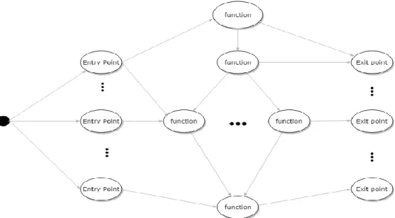
This model should be able to leverage the object oriented programming paradigm as most of the deep learning projects provide an interface in Python. The user should be able to see all the entry points and exit points for all possible runs in an open source project. Based upon the length of the run and other statistics, the user should be able to decide on the optimized one. As these projects are gigantic, the solution provided should be efficient, easily scalable, user friendly and self-sustaining.

1.3 Proposed Solution

To auto generate the solution to machine learning problems from the existing models, it is important to know the flow of logic and semantics of the code. In this thesis, it has been decided to use deep learning technologies to design a model which is capable of analyzing the given code and its behavior static call graph perspectives. It will be executed in a defined finite number of iterations. In the first iteration, all the metadata will be extracted. This metadata can be different entities of Object Oriented Programming. These can be methods, classes, functions, etc. Once the metadata is extracted then the call graph is generated on top of it.

First one is static call graph, which represents how the deep learning is done at every stage with respect to source code. It is a generalization of the source code with entry points and exit points. Here all the combinations of paths from the entry point to exit point are shown. Static call graphs are best in their own way, in terms of exposure, they can add value to

application users.

Furthermore, for any organization, it will be interesting to adapt to a system which can train people on open source projects quickly. Users should have an application where they can observe static call graphs for any open source project and can make vital decisions on the call graphs. They should be able to understand the important clusters in the project. Ease of enhancement should be facilitated with the help of these call graphs. Optimal paths selection should be possible with the help of these call graphs.

The user should be able to see the various entry points, middle ones, and the exit ones. Based on the performance and the shortest path between an entry and an exit point User can easily learn and start making a decision on what can be the best program for any particular goal.

CHAPTER 2

BACKGROUND AND RELATED WORK

2.1 Terminology

In this chapter, the key terms related to software system are introduced and their interpretations in the context of this paper are defined.

Call Graph [2]: It is a control flow graph. It is represented using edges and nodes. The edges represent the function calls between various subroutines of the same program. The nodes represent the specific subroutines. It facilitates the human understanding of the code. It tracks the way the values are passed between various functions. Figure 1 displays such a sample call graph.

Dependency Graph: It is a directed graph showing the various dependencies among different objects or entities of a software system. The edges are directed from one node to another.

Static Call Graph: It represents every possible run of the program. The exact static call graph is an undecidable problem, so static call graph algorithms are generally over approximations. That is, every call relationship that occurs is represented in the graph, and possibly also some call relationships that would never occur in actual runs of the program.

AnyTree [3]: It is one lightweight and powerful tree data structure in python. It simplifies the representations and traversal through trees. One needs to create nodes and can provide the parent node as the parameter. It can be used as plugins as well.

NetworkX [4]: It is the basic python library used for graph creation which can be later visualized using tools such as Graphviz, Gephi, and Cytoscape. Various graph operations like searching, traversing are easy to implement using it, and the graph can be converted to the desired format as needed by graph visualization tools.

2.2 Related Work

The proposed model’s function is similar to the way in which python programs are represented using different call graph construction algorithms.

Pycallgraph[5]: It is an open source python utility that creates call graph visualizations for Python applications in a dynamic way. The call graph generated by it depicts the way in which the program/process is getting executed and the various function calls happening at each line of code at execution time. In addition, it also represents the execution time at each node and the total number of calls being made. It is unreadable if being called at a very high level and hence needs to be wisely used in specific areas of the source code. It is a directed colored

graph and uses Graphviz library. It is mainly used for dynamic call graph generation.

Pyan [6]: It is static call graph generator for python source codes originally written by Edmund Horner, and then enhanced by Juha Jeronen adding colorization and other features. It generates approximate call graphs for python programs. Pyan takes one or more Python source files, performs a (rather superficial) static analysis, and constructs a directed graph of the objects in the combined source, and how they define or use each other. The graph can be output for rendering by GraphViz(graph visualization tool).

Prashanth Ellina [7] also suggested visualization for a specific python module. The construct_call_graph code written by Prashanth Ellina module provided this framework and can easily interpret the unwanted parts in code that are not useful anymore. It involves removing all the globals and to use explicit variables instead. It works on the parser, an inbuilt library of python which constructs a syntax tree for a given python module. This is a nicely written code, which requires manual intervention and useful for around 10k+ lines of code with 300-400 functions calls. The same was executed on one Tensorflow file and the followings results were achieved. However, it is not scalable for bigger projects.

Cloud AUTOML [8]: It was recently published in alpha stage in January 2018. It works on the principle of state of the art transfer learning and helps the developers with limited expertise in the field of machine learning, to create a custom model to train complex own data to solve personal use cases. DP-Miner [9] proposed a similar approach to discover design patterns using matrix representation of structural characteristics of the software system.

Table 1 in the next page lists all the major approaches to the problem statement and the comparison of them in terms of coverage and the type. By coverage, it means that whether one package, module or all packages will get covered or not by the specified existing framework

or not. Type can be of two types: static and dynamic. Static will generate static call graph and dynamic will produce dynamic call graph.

Table 1: Comparison of various tools mentioned in related work Existing

Framework Type Coverage

Pyan Static Set of files in one package

Pycallgraph Dynamic User program throws an error in case of Tensorflow sample programs as Triangulation error

Inspect

Python Dynamic

Manually need to be inserted at every method call in program.

Prashanth Ellina Solution

CHAPTER 3

PROPOSED FRAMEWORK 3.1 Overview

To develop a new model from the existing models, it is important to know the flow of logic and semantics of the code. In this project; it has been decided to use deep learning technologies to design a model which is capable of analyzing the given code and its behavior from the given perspectives.

It is static call graph which represents how the deep learning is done at every stage with respect to source code. It is a generalization of the source code with entry points and exit points. Here, all the combinations of paths from the entry point to exit point are shown.

Furthermore, for any organization, users should have an application where they can observe these call graphs for any open source project and can be trained effectively. The user should be able to see the various entry points, middle ones, and the exit ones. Based on the performance and the shortest path between an entry and an exit point User can easily learn and start making a decision on what can be the best program for any particular goal. The optimization of the code can be done in the least amount of time using this framework. It will enhance their productivity. Moreover, this adds to the in-depth understanding of the developers for any given open source project.

3.2 Model Architecture

The architecture diagram shown in Figure-2 explains how the proposed intelligent model works. The model takes a deep learning model source code as input. The source code is analyzed to determine functionality in terms of the package structure, class structure, and

module structure. The code with similar functionality and structure is grouped together into a cluster to reduce complexity. The next step will provide an interesting visualization to these clusters in form of static call graphs.

Figure 2: Architecture of proposed model

3.2.1 Uniqueness of the Model

Deep learning projects use artificial neural network models that are employed in order to solve a wide spectrum of problems in optimization. Some of the commonly used models are multilayer perceptron (MLP) network and its variations (the time-lagged feedforward network (TLFN)), the generalized radial basis function (RBF) network, the recurrent neural network (RNN) and its variations (the time delay recurrent neural network (TDRNN)), and the counter propagation fuzzy-neural network (CFNN).[10]

These models work differently. CNN Model will learn to recognize patterns called components (e.g., methods of a class) and learn to combine these components to recognize larger structures (e.g., classes). While CNN Model looks for the same patterns on all the subfields, RNN Model feeds the hidden layer of the previous step as an additional input to the

next step (e.g., recognizes the sequence of the method calls).

It is very important to know which of these models will be suitable for the proposed model. The project focusses on providing the information of the type of artificial neural network model used in a particular open source project.

3.3 Code Structure Analysis (CSA)

This is the first fundamental step in the construction of call graph generation. It is implemented for python based projects but can be extended to other programming languages as well. It takes the root directory path as input and then walks on all the files and directories within that directory. It checks for each word in the file against the rule engine and adds the important words to the dictionary. Dictionary is a key value data structure. Here, key will be the file name and the value will be a list of words. These list of words are clustered into Packages, Classes and Functions in accordance with rules defined by the model rule engine. This list of words is returned as a dictionary to the call graph generation module. Algorithm CSA can be defined as follows:

Algorithm 1: CSA

REQUIRE: root directory to perform analysis on INPUT: root directory

OUTPUT: Dictionary: Imported Packages, Classes, and Functions 1 Initialize rootnode ← rootDirectory

2 fileFxnDictionary ← {} 3 fileClassesDictionary ← {} 4 fileImportsDictionary ← {}

5 for each directory in root directory 6 do{

7 for each file in directory 8 do {

9 if fileExtension is not .py 10 then continue

11 for each word,nextWord in file 12 do { 13 for each rule in ruleEngine

14 if rule(word, nextWord) = True 15 if word = functionKeyword 16 updateDict(fileFxnDictionary,file,nextWord) 17 if word = importKeyword 18 updateDict(fileClassesDictionary,file,nextWord) 19 if word = classKeyword 20 updateDict(fileImportsDictionary,file,nextWord) 21 End

It is the core algorithm of this project. It publishes the core fundamental components of python projects. These components are Packages, Modules, Functions, and Classes. As seen in the diagram, one can understand the level they encapsulate within them. For example, Packages consists of sub-modules which further can consist of classes and functions. Figure 3

illustrates the various entities extracted by code structure analysis. 3.3.1 Package structure

The package is the fundamental unit and the top entity in python. It is a directory which will always have a __init__.py special module in it. It is a self-contained module. Every package is a module but every module is not a package. It is visualized using d3.js javascript.

Figure 3: Fundamental structure of Python project Packages

Sub Modules

Classes

3.3.2 Module structure

A python module is simply a python file with extension .py and it comprises of Classes, Functions, global variables. It can be imported into other modules as well and then it is treated as a namespace. A namespace is a dictionary which maps module name to object.

A module allows you to logically organize your Python code. Grouping related code into a module makes the code easier to understand and use. A module is a Python object with arbitrarily named attributes that you can bind and reference.

Simply, a module is a file consisting of Python code. A module can define functions, classes, and variables. A module can also include runnable code. Figure 4 displays a sample module.

Figure 4: Sample module view from Tensorflow (python open source project)

3.3.3 Class structure

Classes provide a way to encapsulate data and functions into one unit. Python is an object-oriented language and provides an object-oriented mechanisms with minimum semantic support. It is defined using class keyword and subclasses other parent classes as a parameter.

Figure 5: Sample class view from Tensorflow(python open source project)

3.3.4 Functions structure

Python functions are a simple callable object in Python. A callable object is an object that accepts parameters, performs actions, may call other callable object and can possibly return a value.

3.4 Feature Extraction

This is the second iteration. In this iteration, the caller functions are retrieved from the first iteration. The next step is to determine the callee functions. Now any function call in python with happen with open braces. So all the words inside the caller functions are traversed and then each word will be analyzed. The stop words will be eliminated at this stage.

Figure 7: Steps of feature extraction

Apart from regular python keywords, unit test case function like assertEquals, assertNotEquals, etc. also need to be excluded. The unit test cases are developed as part of source project to perform unit testing and it does not contribute to the framework usage in outside world. That is why there is no need to include them as part of the proposed model.

One more thing is observed in this iteration and that is the function names are too long to display as a node in the call graph. Hence, each function is abbreviated. The abbreviation is

Caller

functions • From Iteration1

Keywords list with calling

notation

• In python function call happens with open brackets

Stop words

removal • Python inbuilt functions and keywords have been removed

Abbreviate each function for better visualization Create caller callee graph

done incrementally for every unique function name encountered. This will simplify the visualization in later stages. Once the child function of the caller function is identified, it is added as an edge to the networkX graph. The nodes are caller and callee function names. The direction of the edge shows the caller to callee relationship. The figure 7 shows the various steps involved in the second iteration.

3.4.1Caller/Callee View

The caller callee view displays the information of the current function with its parent and child functions. Figure 8 illustrates the caller-callee matrix in the form of an undirected graph.

Figure 8: Caller callee view

The left most of the grid shows the entry point for all possible executions in the source code and the rightmost shows all the exit points for all the possible executions. The middle layers will show the parent and child of respective layers of current functions.

3.5 Clustering

This is the third iteration in the proposed model framework. Figure 9 shows the steps involved on a broader level. Once the caller-callee graph is created, the various paths from one end to another end are identified. A path shows the overall run from one entry point to one exit point. A list of paths is generated. They vary in number according to the project size. The more the size the more is the number of paths.

After the list of paths is generated, they are encoded in binary values. The respective functions, which are present in a particular path are converted to 1 or 0 value. It will be explained in more detail in further steps. Once the encoded matrix is generated, the similarity between various paths is measured. The similarity matrix is passed on to various clustering algorithms and then it is visualized. The clustering data is stored in JSON format to visualize using d3.js javascript. Figure 9 shows the various steps involved in the clustering process.

Figure 9: Steps in iteration 3 – clustering

Path generation

Encode

Similarity Matrix

Clustering

Algorithms

Visualize

3.5.1 Path generation

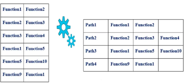
The input to this step is caller callee matrix in the last step. Figure 10 describes the whole process. Here, the input is the caller and callee information in the form of edges of a graph and it gets converted to corresponding paths. As function 2 is calling function 3 and function 3 is calling function 4, it can be considered as one path.

Figure 10: Input and output sample for path generation

The output for this step is the path list as p1, p2, p3 and so on. Python NetworkX library is used for this computation. The below algorithm explains the overall process.

Algorithm 2: PG

REQUIRE: caller callee graph INPUT: G -> caller callee graph OUTPUT: List of Paths <p1,p2,p3>

1 for each node in G 2 do{

4 Add node to sinkNodeList 5 if indegree = 0

6 Add node to sourceNodeList

7 Calculate each edge from source node and sink nodes one by one to create a path Path1 ={ function 1, function 2, function 3,function 4………..}

8 Add path to list of paths

9 End

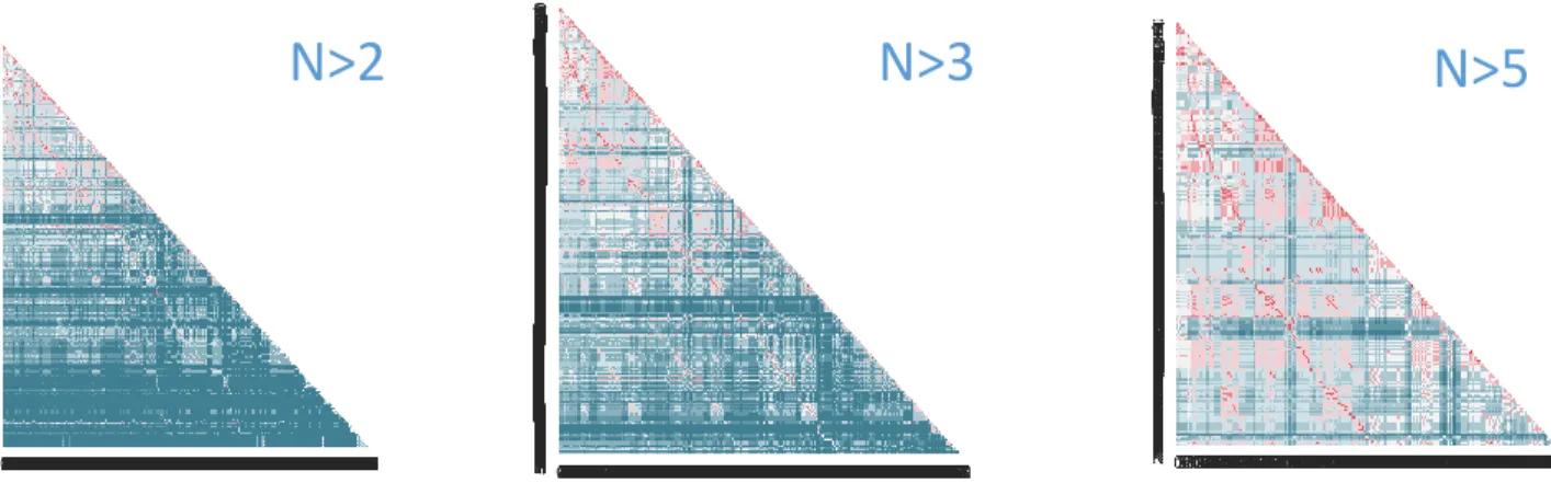
As the list of paths are huge and around 30 percent of the paths have only two nodes, it was making the further operations cumbersome and time-consuming. Even for a small project like Keras, the number of paths tend to be 3000+. So it is most important to decide how many paths to consider for further calculations. Figure 11 shows the percentage of paths and their similarity versus distinct features. In the figure 11where n > 2, where n is the number of functions/nodes in a path, the lower region shows distinct features and hence cannot contribute much to the clustering algorithms. It will obviously result in more and more clusters. Similarly, the n > 3 have around 50% , below the region in blue color. It depicts that most of the paths in lower region are unique. However for n > 5 one can observe more red color and chances of similarity will be high and good clusters will be formed.

N>2

N>3

_N>5

3.5.2 Encoding Paths

List of paths generated in the previous step needs to present in form of binary values to make the calculations easy for further steps. It is inspired by one hot encoding [11]. One hot encoding is a process to convert categorical values to a form, mainly binary, to provide it as input to machine learning algorithms to perform better clustering. It incrementally increases the categorical value for each unique encountered categorical values.

In the same way, this step, instead of incrementally increasing the categorical values, 1 and 0 are used to show the respective function existence in the path. That means for path 1 if function 1 is present, then function 1 value will be 1 in the dataset generation. All other functions which are not present will be marked zero. Figure 12 explains the whole process. As one can visualize, on the left-hand side the path matrix is given. On the right-hand side, the output generated using encoding paths algorithms has been given.

One observation made during this process is that some of the functions are not present in any of the paths. These features are incapable of producing any results using machine learning algorithms. They can be called as Orphan functions and hence have been removed from the overall process.

3.5.3 Similarity Matrix

Once the encoded matrix is generated in the above step, the various paths are checked for similarity with each other. There are various similarity measures/distance available like Euclidean distance, Manhattan distance, Minkowski distance, cosine similarity[12], Jaccard similarity and so on [13]. It is the basic building block in many computations related to deep mining domain like clustering, classification, recommendation engines and anomaly detection. It is very intuitive and measures how two things in a dataset can be similar to each other. They are heavily used nowadays in Machine learning domain.

A set is an unordered collection of objects and is always unique. A set cannot have duplicate elements. The number of objects in a set is called Cardinality. The intersection of the sets (A ∩ B) is defined as the common elements in both the sets. On the other hand union of the sets (A ∪ B) is defined as all the elements which are in either set.

The selection of the similarity measure also depends on dataset passed on as input. This step utilized Jaccard similarity measure as defined in below quote. Here, each feature in a dataset is treated as an object in the set.

“The Jaccard similarity measures the similarity between finite sample sets and is defined as the cardinality of the intersection of sets divided by the cardinality of the union of the sample sets.” [14]

Jaccard similarity can be represented using below formula.

Using the above formula in figure 13, the similarity matrix has been computed. The similarity matrix is a representation of similar sequences in a data series in a graphical manner or matrix. Figure 14 denotes how encoded matrix is transformed to similarity matrix.

Figure 14: Input and output for similarity matrix

In order to construct similarity matrix, the data set has been considered as an ordered sequence of paths and converted to feature vectors as <path1,path2,path3,path4………pathn>

where each vector pathdepicts the position of the relevant feature in the dataset series. Here, the pair of feature vectors is taken at once and then the similarity measure is used to check the similarity.

Jaccard similarity (A, B) = Intersection (A, B) / Union (A, B) = (A ∩ B) / (A ∪ B)

Figure 13: Jaccard similarity formula

S (i, j) = similarity (pathi, pathj) where i, j € (1, 2,……..n)

The formula in figure 15, provides the formula involved for calculating each cell value in the similarity matrix. Here, S (i, j) denotes the value of the ith _{row and j}th _{column in the}

similarity matrix.

3.5.4 Clustering algorithms

Clustering [15] is the process of grouping together similar elements. Each group is called a cluster in the field of data mining. Here, elements are paths and the similarity between them is defined in the above iteration. There are various clustering algorithms used to cluster data. They are based on different principles.

Figure 16: Clustering input and output

Various clustering algorithms are available in data science and can be classified broadly as follows:

Centroid-based clustering: It is based upon the principle that each cluster can be

represented by a central vector also known as the centroid. A popular example of this is K-means clustering algorithm. Mostly they require optimization.

Density-based clustering: It is based on the principle that cluster is the high-density areas than the rest of the datasets. Objects which are present in light dense areas are considered noise and border points. It connects elements in a cluster which share the same density level in the dense area. DBScan is the most popular algorithm for this kind of scenario. A core point is a point if it has more than a specified number of points (MinPts) in specified radius (Eps). A border point has fewer than MinPts within Eps. Noise points are the ones that are not a core point or border point. Below figure 18 illustrates the same. [16]

Figure 18: Density-based clustering [17]

Connectivity-based clustering: It is also known as hierarchical clustering. It is based on the principle that objects which are near to each other are more similar than the objects which are at more distance. It can be represented using dendrogram.

Hierarchal clustering (Agglomerative) consider each data point as a single cluster and then repeatedly combine the nearest two clusters into a single one. The inter-cluster distance is measured by the distance between their centroids. It groups data objects into a tree of clusters

and outputs as a dendrogram.

Figure 19: Hierarchal clustering dendrogram [18]

It is important to understand how the various clustering algorithms, belonging to above mentioned broader categories are implemented. First of all, consider a training set of

x

,...,x

Figure 20: Different distance measures between vector points

Euclidean distance has been used as metrics for distance calculation and is defined as the straight line between the two vectors. Manhattan distance is the absolute differences between the two vector points. Formula representation for each of them can be given in figure 21 and 22 for two vectors X=(x1,x2,……xn) and Y=(y1,y2,……yn).

Figure 21: Formula for Euclidean distance

Figure 22 : Formula for Manhattan distance

KMeans initially picks k centroids to define a cluster. The distance between the point and the centroid is measured and the point is assigned to the closest centroid cluster. The process is repeated for each data point, and for as many iterations till when the previous and the present iterations don’t produce the same result. Algorithm for KMeans [19] can be specified as shown below:

Algorithm: KMeans

INPUT: Data set Rn _{and number of clusters k}

OUTPUT: set of clusters

1 Initialize cluster centroids µ1, µ2,….., µk€ Rn randomly

2 Repeat until convergence: { 3 For every i, set

𝑐(𝑖)_{≔ arg}𝑚𝑖𝑛

𝑗 ‖𝑥𝑖 − 𝜇𝑗‖ 2

4 For each j, set

𝜇_𝑗 ∶= ∑ {𝑐 (𝑖) _{= 𝑗}} 𝑚 𝑖=1 𝑥(𝑖) ∑𝑚 1{𝑐(𝑖) _{= 𝑗}} 𝑖=1 5 } 6 End

Minimum batch KMeans is another faster enhancement of KMeans algorithm and works very well on huge datasets by taking only a subset as training and then efficiently

𝑑𝑖𝑠𝑡(𝑋, 𝑌) = √(𝑥₁− 𝑦₁)2_{+ ⋯ + (𝑥}

𝑛− 𝑦𝑛)2

generalizing at the whole dataset. The results are quite accurate and much faster computed. Algorithm for it can be specified below:

Algorithm: Minimum batch KMeans [17]

INPUT: k, mini-batch size b, iterations t, data set X OUTPUT: set of clusters

1 Initialize each c €C with an x picked randomly from X 2 v ← 0

3 for i =1 to t do

4 M ← b examples picked randomly from X

5 for x € M do

6 d[x] ← f ( C, x) //cache the center nearest to x 7 end for

8 for x € M do

9 c ← d[x] //get cached center for this x 10 v[c] ← v[c] +1 // update per-center counts 11 n ← 1/v[c] //get per-center learning rate 12 c ← (1- n)c+nx //take gradient step

13 end for 14 end for

DBScan is a density-based clustering algorithm and stands for Density-Based Spatial Clustering Application. Density refers to a number of data points in a vector space D within a specified radius (Eps). It discovers clusters of arbitrary shape with core points, border points, and noise points. DBScan algorithm can be defined as follows:

Algorithm: DBScan

INPUT: n objects to be clustered and global parameters Eps, MinPts. OUTPUT: set of clusters

1 Initialize point P //arbitrary selection 2 Sp← 0

3 for k € n do 4 for i € n do

5 if Pi = density-reachable(P,Eps.,MinPts.)

6 Sp← Sp + Pi

8 Output cluster Sp

9 end for 10 end for

Single linkage hierarchal clustering used as part of the thesis, has been picked up from the seaborne python package. The single linkage can be defined as the shortest distance from any member P of one cluster Ci to any member P’ of the other cluster Cj. There are also

other types of linkage available, like complete linkage and average linkage. Single linkage distance formula can be described as follows in figure 23:

Figure 23: Single linkage distance formula

Algorithm for hierarchical clustering can be specified as follows: Algorithm: Hierarchical clustering [17]

INPUT: a set X of objects {x1, x2,…,xn}and a distance function dist(c1,c2)

OUTPUT: set of clusters 1 for i ← 1 to n do 2 ci ← {xi} 3 end for 4 c ← {c1,…,cn} 5 L ← n+1 6 While C.size > 1 do 7 (𝑐𝑚𝑖𝑛1, 𝑐𝑚𝑖𝑛2) = 𝑚𝑖𝑛𝑖𝑚𝑢𝑚 𝑑𝑖𝑠𝑡(𝑐1, 𝑐2) 𝑓𝑜𝑟 𝑎𝑙𝑙 𝑐𝑖, 𝑐𝑗 𝑖𝑛 𝐶 8 Remove 𝑐_{𝑚𝑖𝑛1} 𝑎𝑛𝑑 𝑐_{𝑚𝑖𝑛2}𝑓𝑟𝑜𝑚 𝐶 9 Add {𝑐𝑚𝑖𝑛1, 𝑐𝑚𝑖𝑛2} to C 10 L ← L + 1 11 end while

Affinity Propagation (AP) is a relatively new clustering algorithm and is based on the concept of "message passing" between vector points. It does not require the number of clusters

to be determined or estimated before running the algorithm. It can be specified as follows:

“An algorithm that identifies exemplars among data points and forms clusters of data points around these exemplars. It operates by simultaneously considering all data point as potential exemplars and exchanging messages between data points until a a good set of exemplars and clusters emerges.”[20]

Based on the above information, there are a few prerequisites for clustering algorithms. They are summarized in table 2 one by one:

Table 2: General information about clustering algorithms [21]

Method name

Parameters Scalability Usecase

K-Means number of clusters

Very large n_samples, medium n_clusters withMiniBatch code

General-purpose, even cluster size, flat geometry, not too

many clusters Affinity propagation damping, sample preference

Not scalable with n_samples

Many clusters, uneven cluster size, non-flat geometry

Minimum Batch

K-Means

number of clusters

Very large n_samples, medium n_clusters withMiniBatch code

General-purpose, even cluster size, flat geometry, not too

many clusters

To reduce computation time DBSCAN neighborhood

size

Very large n_samples, medium n_clusters

Non-flat geometry, uneven cluster sizes

Hierarchical number of clusters

large n_samples and n_clusters

Many clusters, possibly connectivity constraints

As per the table 2, the different clustering algorithms that have been used for this project are shown. They also show what are the different parameters required for each one of them. For some of them a number of clusters are required, for others neighborhood size which tells what distance to look for between current element and the other element in the vector space while clustering.

The most important deciding factor while clustering is what will be the value of these parameters. The better the parameter, the better the clustering result. There are various ways to validate the clustering parameters. As one can manually see the clustering results and can understand that what paths in the source code tends to be similar, hit and trial method can be used to determine the different parameters like the number of clusters, neighborhood size and etc. Using hit and trial manually edit the parameters to understand that the clusters created are of the desired type or not.

One of the most popular ways is to use Silhouette coefficient [22]. It contrasts the average distance to elements in the same cluster with the average distance to elements in other clusters. This index works well with various clustering algorithms and is used to determine the optimal number of clusters. The range for its value is [-1, 1]. The higher the value of the coefficient, the samples are not well clustered and the less the value the samples are well formed very near to decision boundary. Negative values of silhouette coefficient indicate that samples are entered into wrong clusters and there is a potential problem in the parameters

selection.

Silhouette Coefficient = (b - a) / max (a, b) where a= mean intra-cluster distance b= mean nearest-cluster distance

The Silhouette Coefficient is calculated using the mean intra-cluster distance (a) and the mean nearest-cluster distance (b) for each sample. The Silhouette Coefficient for a sample is given in figure 28. Remember, b is the distance between a sample and the nearest cluster that the sample is not a part of.

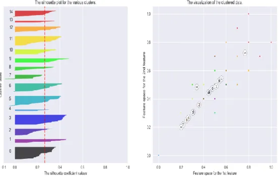
In the figures 29,30,31,32 one can see on the left-hand side the thickness of various clusters and on the right-hand side various clusters are visualized. Table 3 lists the values of silhouette coefficient for a different number of clusters for one of the open source project and one can see the score does not have much deviation.

Table 3: Silhouette Coefficient for different number of clusters

number of clusters score

2 0.257592 3 0.268325 4 0.250305 5 0.256854 6 0.25752 7 0.278742 10 0.273551 11 0.270473 12 0.286374 15 0.265885 20 0.284066

For a number of clusters, 5, 10, 15, 20, the silhouette coefficient can be plotted and are shown in below figures 25-28 for one of the sample project. The thickness of the clusters on the left-hand side helps in selecting the optimal number of clusters. For this particular sample

case as shown in figures on next pages, number of clusters selected is 15.

Figure 25: Silhouette analysis for KMeans clustering for a number of clusters =5

Figure 27: Silhouette analysis for KMeans clustering for the number of clusters =15

Based on the all of the above analysis, the table 4 listed values have been picked up for our experimentation. The below table details the various values that have been used for different clustering algorithms. Out of all, the Hierarchical have proved the best results based upon the output and hence, it is the best choice among all for our projects. The number of clusters, in this case, is optimized for better results. Other algorithms are also detailed and shown in the below table.

Table 4: Parameter values for different clustering algorithms

Algorithm Name Parameters Value

K-Means number of clusters 10

Affinity propagation

damping,

sample preference

None -50

Minimum Batch K-Means number of clusters 15

DBSCAN neighborhood size

Minimum_Samples

2 10

Hierarchical number of clusters Optimized for different source projects

3.6 Static Call Graph Generation

This is the last iteration of the proposed model. Here first the AnyTree created in the previous iterations is converted to DOT file and the given DOT file is visualized using Graphviz library.

Figure 29: Static call generation steps

Any user program can be analyzed using a call graph, which helps put together a basic analysis of the relationship between the procedures and their flows. For understanding, if a rooted directed graph is plotted, where G= (V, E), vertices represent a method v as V and a method call from method v to method u is represented by an edge E where E= (v, u) [23].

• AnyTree

• DOT file

generation

• Visualize

using

Graphviz

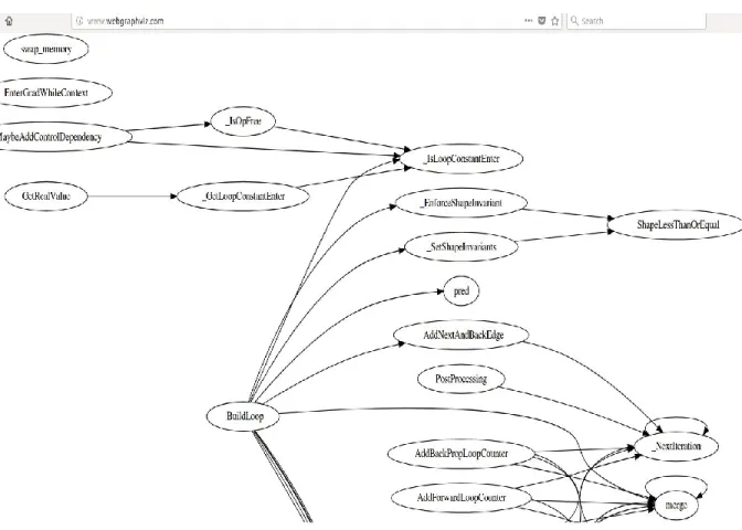
Call graph illustrates the call relationship between different procedures. In simple words, a call graph is the graphical representation of the execution logic of the program. It can tell the various dependencies between the different entities of the classes as shown in figure 30.

A Single caller, a method presently can have multiple possible callers. In case there is no invocation inside a method body, it could mean that the corresponding set has a size 0, meaning that particular method is not called. To write logic where a call graph can generate a more accurate outcome, or add an increased degree of precision, would require creating a more complex algorithm at a cost of lengthier calculations and increased usage of memory.

Figure 30 shows how the call graph visualization has been done using Graphviz. Graphviz is open source graph visualization software used to represent the structural information contained in the DOT file. In order to visualize it, DOT file is generated based upon all the information extracted in the previous iterations. A DOT file is a graph description language and usually, have .dot extension. It can be undirected or directed in nature. In our case, since the calling relationship is important, the directed version is used in DOT file.

Figure 32 details one of the sample DOT graph. It starts with graph keyword and rankdir tells about the orientation of the graph, which can be top to bottom or left to right. The next lines tell about the various calling relationships present in the source code. For example, a is calling b, c, d in given figure 32 case and so on. As part of this iteration in order to generate DOT file, AnyTree has been used. Below figure 32 details, the sample Node Tree implemented as part of this thesis.

CHAPTER 4

RESULTS AND EVALUATION

4.1 Introduction

The evaluation conducted on the different open source projects are described in this chapter, along with testing environments. Due to large nature for one of the open source projects, the memory needed for algorithms executions needed to be increased to 9 GB during runtime execution. This chapter will discuss the projects selection, configurations needed and what was the output for each iteration for each selected project.

4.2 Selection of Deep Learning Projects

Given the enormous amount of available resources today, many researchers need to figure out the path to machine learning. The field is evolving rapidly and one needs to be in constant with the evolving speed of deep learning domain. In that view, it was important to understand the various resources available in this domain. Below are the top 20 deep learning projects available in Github as per the study in table 5.

Table 5 lists all the deep learning projects which are popular currently and a small description about each one. The table 5 also lists the programming languages they provide for. Many of the deep learning projects are providing support in two or more languages, which makes it easy for the user to select the language of their choice to implement in their solution.

Table 6 presents the various deep learning projects selected from GitHub. It also includes the contributors, the number of commits and the stars (rating) given to them by GitHub users. The count of stars reveals the popularity among enthusiastic machine learning developers and the number of commits signifies the changes occurred overall in the project in order to enhance or improve.

Table 5: Top Deep Learning projects [24]

Name Description Language Support

Tensorflow works on tensors and data flow graphs _{to implement machine learning} Python, Java, Go, C scikit-learn built on NumPy, SciPy, matplotlib and _{simple, efficient tool for data mining} Python

Keras

high-level neural network API utilizing Tensorflow, Theano or

CNTK

Python

PyTorch promotes tensors and Dynamic neural

networks Python

Theano define, optimize and evaluate

mathematical expressions Python, C++ Gensim provides scalable statistical semantics _{for text documents} Python

Caffe deep learning framework with good _{speed, expression, and modularity} C++ library with Python Chainer implements neural networks and state _{of the art models} Python

Statsmodels easy to do statistical models and tests Python Shogun

easily integrate multiple data representation, classes, and general

purpose tools Python

Pylearn2 use Theano to optimize expression and computations written using Pylearn2 plugins

C++ with Python, Octave, Java / Scala, Ruby, C#, R, Lua

NuPIC

based on theory neocortex called HTM as hierarchical Temporal

Memory

Python with C++ Neon easy to use deep learning library Python Nilearn _{modeling, classification etc. analysis} uses Scikit learn for predictive Python Orange3 provides interactive data analysis

workflows with a large toolbox Python Pymc implements Markov chain, Bayesian _{statistical models etc.} Python Deap Computation Framework for quick

prototyping and parallel mechanism Python Annoy search for points near to query point in

According to Table 6, Tensorflow has taken the first position with the maximum number of contributors. Another one which has gained popularity recently in the year 2018 is Keras, due to simplicity pf coding. PyTorch is also among the top contenders and is a medium sized project. Scikit-learn has been used to do the experimentation as part of this thesis and hence not selected further even after being in top ones.

Table 6: Top Deep Learning statistics as of Apr 1, 2018

Name Contributors Commits Stars

Tensorflow 1409 30843 94671 scikit-learn 1042 22675 27028 Keras 649 4433 27692 PyTorch 582 10492 13419 Theano 329 27963 8080 Gensim 273 3593 6650 Caffe 264 4118 23510 Chainer 158 13463 3629 Statsmodels 149 9877 2724 Shogun 141 16483 2052 Pylearn2 119 7119 2562 NuPIC 84 6594 5537 Neon 77 112 3451 Nilearn 70 6272 383 Orange3 56 9051 1258 Pymc 39 2721 652 Deap 39 1960 1842 Annoy 35 537 3321 PyBrain 32 992 2541 Fuel 32 1116 702

Figure 33 presents the graphical view of the various projects projecting the contributors on the x-axis and commits on the y-axis.

Figure 33: Top 20 Python AI and Machine Learning projects on Github [24]

Hence, considering the popularity factor and better future prospects the following projects have been selected for the experimentation:

 Tensorflow  Keras  PyTorch

4.3 Configuration

4.3.1 Hardware Configuration

As the open source projects tend to be larger, specific hardware requirements are needed as given below:

• Processor: Intel® Core(TM) i7-6700HQ CPU @ 2.60GHz • Operating System: Windows 10 Home , Ubuntu 16.04.1 • OS Type: 64 bit

• Disk: 500 GB SSD

4.3.2 Software Configuration

To implement the proposed solution, the following software and libraries have been used:

• Python 3.5

• Pycharm 2018.1 Community Edition • TensorFlow-gpu 1.0.1 • Numpy Library • MatplotLib Library • AnyTree • ExcelUtility • Sci-kit learn • d3.js 4.4 Experiment 1: Tensorflow

Tensorflow [25] was initially designed and developed by Google as an internal project to solve problems using deep learning and machine learning. It was later made public, making it open source and available for developers. It is an open source library that helps us expose Machine Learning algorithms on a very niche level of program, and assists implement

execution of such algorithms. Executing a numerical calculation with Tensorflow is easy to implement on different systems with varying and diverse systems. Its architecture provides multiple ranges of advantages, specifically for deep neural network models, and used on different API levels and accelerators such as CPU, TPU, and GPU cards. Being flexible makes it possible to have a single API to deploy computations on more than one variety of system, be it mobile or desktop server.

Tensorflow is a layered architecture, in that the flexibility to support new models and system level improvements, makes it easy. To construct a neural network, it utilizes a High-level API. Tensorflow separates its core from the code on various platforms (C++, Python etc) by a separator C API. Other core components of the Tensorflow architecture after are:

 Device Layer  Network Layer  Distributed Master  Dataflow Executor  Kernel implementation.

In Tensorflow, a data graph is used to denote the algorithm where the flow of data is represented by the edges, and the nodes represent the procedures. A data flow graph usually consists of Procedures, Tensors, Variables, and Sessions.

 Procedure: one of the benefits of representing the algorithms, as the graph helps to visualize the connections between the calculations, making it simple and generic to define a procedure. In short, the Graph represents how the data is transformed through the various procedures.

multi-dimensional collection of similar values.

 Variables: Described as persistent, mutable handles to in-memory buffers storing tensors.

 Sessions: Is a special environment in which the execution and evaluation of a procedure take place.

4.4.1 Architecture

Tensorflow is designed by keeping in mind large scale distributed systems. It is quite flexible, in terms of experimentation with different new machine learning models and kinds of optimizations at the system level. Tensorflow runtime is a cross-library platform. Figure 34 describes the architecture of Tensorflow in detail in four layers.

Figure 34: Tensorflow layered architecture [26]

The first layer is Client. It is responsible for defining any kind of computation as a data flow graph. It creates a session and initiates the graph construction mechanism. The second

layer is Distributed, Master. It prunes the graph generated above into subgraphs. These subgraphs represent a small set of computations. This computation is equivalent to different processes which are assigned to different devices or workers and execution is initiated at the worker level. The third layer is worker services (one for each subgraph). It executes the operations, in terms of kernel implementations, as per the hardware configured like GPU, CPU etc. In addition, it interacts with other worker services, as well, to transfer and get outputs of the operations executed by these set of workers. The last layer is the core that is Kernel Implementations. It performs the computation for individual graph operations.

4.4.2 Code Structure Analysis Results

In the first iteration, the system will analyze the different features of the source code. A crawler is created to crawl through each python file to associate the methods with respective packages and classes. There is a total number of 15k+ API available and their respective packages are known. Counts are given in Table 7 as per experiment for the packages, functions, modules, classes and other relevant things in relation to python project.

Table 7: Features statistics using CSA

Entity Count Files 841 Packages 116 Classes 2108 Functions 15758

Other imported modules 13758

There are around 841 python files on which this analysis has been completed. The code ignored all other files than python. The number of packages or directories in the source code is 116. Each of these directories contains init.py. There are more than 2k+ classes. Some of the classes are written for unit testing or another testing. The implementation does not ignore the testing classes or methods. By the number of functions, one can assume the complexity of TensorFlow deep learning project. Also, the number of imported modules are also very high. Here, it is very important to understand that if one module is imported into different files, than it is counted twice rather than once. However, the unique count is 1187. That is, in total there are these many different imports in the whole source project.

First, the CSA will walk through all the modules and packages in the Tensorflow source code. The following graphical interpretation of the package structure has been done using d3.js JavaScript. It shows the exact python package name present at each level. As the graph was quite huge, only a small portion is shown of the same. As one can see, Tensorflow is the root further breaking down to root, config folders and the process goes on.

4.4.3 Features extractor

After walking through the different files, the following information has been extracted. There were a few observations discovered.

There are many test files with _test.py name and they contains unit test cases to test individual code of source code with associated control data, usage, and operating procedures. A test case can be created by the subclassing unit test. TestCase and different assert statements are used for the same. These can be ignored, as they do not contribute to the machine learning models.

Table 8: Tensorflow statistics

Files_count Import_Count Class_count Function_count

Only Test Files 557 7045 1387 9690

Without Test Files 632 6737 721 6068

Total 1189 13782 2108 15758

Table 9 details the paths statistics for Tensorflow. There are a total of 73805 paths and out of them, only 3304 paths have nodes greater than 5. They are used further for clustering.

Table 9: Tensorflow path statistics

Total number of Paths 73805

Total number of Paths with nodes > 5 3304

These paths are stored in .xlsx(excel file). Below figure 36 shows the sample view of

the file:

Figure 36: Nonabbreviated view of paths for Tensorflow

4.4.4. Similarity Matrix

The paths generated using feature extraction phase have been clustered and plotted using various algorithms. Below are the results in the two categories. First, all the paths are analyzed and clustered. On the left-hand side, one can visualize the similarity matrix. The more the red color the more is the similarity between x-axis and y-axis. On both the x-axis and the y-axis, the path number is represented. The scale used is 0 to 1 to represent similarity between

After clustering

Figure 38: Overall heatmap representation of Tensorflow after clustering

After clustering

two paths. Here 0 represents blue color which means no similarity and red represents value 1 which means high similarity. As the number of paths is huge, only first 50 paths are also analyzed for better visualization. As one can see, on the right-hand side of figure 39, the red paths got clustered together using Hierarchal clustering and shown using dendrogram. Paths 39, 36, 31, 33, 10, 38 and 8 can be clustered into one group. The other one is on the extreme right from Path 19 to path15.

Other clustering algorithms were run on the Tensorflow source code and visualized using d3.js. The following are the results for the same. In case of Tensorflow Minimum Batch K Means produced better clusters than others and looks more distinguishable and readable.

Figure 40: Clustering visualization of Tensorflow

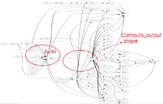
4.4.5 Call graph

The call graph was generated and visualized using Graphviz as shown in figures 41 and 42. The number of nodes is very high as TensorFlow is quite a big project. The view has been divided into two parts. The left-hand side is shown in figure 41 and the right-hand view is shown in figure 42.

4.5 Experiment 2: Keras

Keras [27] is an open source project developed using Python and run on top of TensorFlow, CNTK or Theano. It has recently become popular and facilitates high-level neural networks API. Use Keras if you need a deep learning library that allows for easy and fast prototyping (through user friendliness, modularity, and extensibility) and supports both convolutional networks and recurrent networks, as well as combinations of the two. It runs seamlessly on CPU and GPU. Projects written using Keras are user-friendly, modular, can be easily extended.

4.5.1 Code Structure Analysis Results

After running CSA algorithm the below information is extracted. Keras is a small size deep learning project in comparison to Tensorflow, almost quarter in size.

Table 10: Keras statistics

Entity Count

Files 164

Packages 145

Classes 195

Functions 1933

Other imported modules 1750

Unique imports 164

There are around 164 python files on which this analysis has been done. The code ignored all other files than python. The number of packages or directories in the source code is 145. Each of these directories contains init.py. There are around 195 classes. Some of the classes are written for unit testing or another testing. The implementation does not ignore the testing classes or methods.

4.5.2 Features extractor results

After walking through the different files, the following information has been extracted. There were few observations discovered about this. There are many test files with _test.py name and they contains unit test cases to test individual code of source code with associated control data, usage, and operating procedures. These can be ignored as they do not contribute to the machine learning models.

Table 10 details the paths statistics for Keras. There is a total of 73805 paths and out of them, only 3304 paths have nodes greater than 5. They are used further for clustering.

Table 10: Keras path statistics

Total number of Paths 4324

Total number of Paths with nodes > 5 237

Maximum Length of Path 10

These paths are stored in .xlsx(excel file). Below figure 43 shows the sample view of the file: