System Architecture for Wireless Sensor Networks
by
Jason Lester Hill
B.S. (University of California, Berkeley) 1998 M.S. (University of California, Berkeley) 2000
A dissertation submitted in partial satisfaction of the requirements for the degree of
Doctor of Philosophy in Computer Science in the GRADUATE DIVISION of the
UNIVERISY OF CALIFORNIA, BERKELEY
Committee in charge: Professor David E. Culler, Chair
Professor Kris Pister Professor Paul Wright
The dissertation of Jason Lester Hill is approved:
Chair Date
Date
Date
University of California, Berkeley Spring 2003
System Architecture for Wireless Sensor Networks
Copyright 2003 by Jason Lester Hill
Abstract
System Architecture for Wireless Sensor Networks by
Jason Lester Hill
Doctor of Philosophy in Computer Science University of California at Berkeley
Professor David Culler, Chair
In this thesis we present and operating system and three generations of a hardware platform designed to address the needs of wireless sensor networks. Our operating system, called TinyOS uses an event based execution model to provide support for fine-grained concurrency and incorporates a highly efficient component model. TinyOS enables us to use a hardware architecture that has a single processor time shared between both application and protocol processing. We show how a virtual partitioning of
computational resources not only leads to efficient resource utilization but allows for a rich interface between application and protocol processing. This rich interface, in turn, allows developers to exploit application specific communication protocols that
significantly improve system performance.
The hardware platforms we develop are used to validate a generalized architecture that is technology independent. Our general architecture contains a single central
controller that performs both application and protocol-level processing. For flexibility, this controller is directly connected to the RF transceiver. For efficiency, the controller is
supported by a collection of hardware accelerators that provide basic communication primitives that can be flexibility composed into application specific protocols.
The three hardware platforms we present are instances of this general architecture with varying degrees of hardware sophistication. The Rene platform serves as a baseline and does not contain any hardware accelerators. It allows us to develop the TinyOS operating system concepts and refine its concurrency mechanisms. The Mica node incorporates hardware accelerators that improve communication rates and
synchronization accuracy within the constraints of current microcontrollers. As an approximation of our general architecture, we use Mica to validate the underlying architectural principles. The Mica platform has become the foundation for hundreds of wireless sensor network research efforts around the world. It has been sold to more than 250 organizations.
Spec is the most advanced node presented and represents the full realization of our general architecture. It is a 2.5 mm x 2.5 mm CMOS chip that includes processing, storage, wireless communications and hardware accelerators. We show how the careful selection of the correct accelerators can lead to orders-of-magnitude improvements in efficiency without sacrificing flexibility. In addition to performing a theoretical analysis on the strengths of our architecture, we demonstrate its capabilities through a collection of real-world application deployments.
_______________________________________ Professor David Culler
Table of Contents
Table of Contents... i
List of Figures:... iv
Chapter 1: Introduction... 1
Chapter 2: Wireless Sensor Networks ... 10
2.1 Sensor network application classes... 11
2.1.1 Environmental Data Collection... 11
2.1.2 Security Monitoring ... 14
2.1.3 Node tracking scenarios ... 16
2.1.4 Hybrid networks... 17
2.2 System Evaluation Metrics ... 17
2.2.1 Lifetime... 18
2.2.2 Coverage ... 19
2.2.3 Cost and ease of deployment ... 20
2.2.4 Response Time... 22
2.2.5 Temporal Accuracy... 22
2.2.6 Security ... 23
2.2.7 Effective Sample Rate... 24
2.3 Individual node evaluation metrics ... 25
2.3.1 Power ... 26 2.3.2 Flexibility... 26 2.3.3 Robustness ... 27 2.3.4 Security ... 28 2.3.5 Communication... 28 2.3.6 Computation... 29 2.3.7 Time Synchronization... 30
2.3.8 Size & Cost ... 31
2.4 Hardware Capabilities... 31
2.4.1 Energy ... 32
2.4.2 Radios ... 37
2.4.3 Processor ... 43
2.4.4 Sensors ... 48
2.5 Rene Design Point... 50
2.5.2 Baseline Power Characteristics... 53
2.6 Refined Problem Statement ... 54
Chapter 3: Software Architecture for Wireless Sensors ... 56
3.1 Tiny Microthreading Operating System (TinyOS) ... 57
3.2 TinyOS Execution Model ... 58
3.2.1 Event Based Programming ... 58
3.2.2 Tasks ... 59
3.3 TinyOS Component Model... 60
3.3.1 Component Types ... 63
3.3.2 Enabling the migration of hardware/software boundary ... 65
3.3.3 Example Components ... 66
3.3.4 Component Composition ... 67
3.3.5 Application Walk Through ... 70
3.4 AM Communication Paradigm ... 72
3.4.1 Active Messages Overview... 72
3.4.2 Tiny Active Messages Implementation ... 73
3.4.3 Buffer swapping memory management ... 75
3.4.4 Explicit Acknowledgement... 76
3.5 Components Contained in TinyOS ... 77
3.6 TinyOS Model Evaluation ... 78
3.7 TinyOS Summary ... 80
Chapter 4: Generalized Wireless Sensor Node Architecture... 82
4.1 Wireless communication requirements... 82
4.2 Key issues architecture must address... 85
4.2.1 Concurrency... 86
4.2.2 Flexibility... 86
4.2.3 Synchronization ... 87
4.2.4 Decoupling between RF and processing speed... 88
4.3 Traditional Wireless Design ... 91
4.4 Generalized architecture for a wireless sensor node... 93
4.5 Architectural Benefits ... 96
4.5.1 Concurrency... 96
4.5.2 Protocol Flexibility and Timing Accuracy ... 100
4.6 Summary ... 100
Chapter 5: Approximation of General Architecture: Mica... 102
5.1 Mica design... 103
5.1.1 Block diagram overview ... 103
5.1.2 Raw radio interface ... 106
5.2 Communication accelerators... 107
5.3 Evaluation ... 109
5.3.1 Concurrency Management ... 110
5.3.2 Interplay between RF and Data path speed... 111
5.3.3 Interface flexibility... 112
5.4 Blue: a follow-on to Mica ... 120
5.4.1 CPU... 120
5.4.2 Radio ... 121
5.5 Summary ... 122
Chapter 6: Integrated Architecture for Wireless Sensor Nodes – Spec... 124
6.1.1 High Level Overview... 125
6.1.2 General Block Diagram ... 126
6.1.3 Radio Back End & ADC Sub blocks ... 134
6.1.4 Digital frequency lock registers ... 135
6.2 Performance ... 138
6.2.1 Start Symbol Detection ... 139
6.2.2 Interrupt Handling Overhead ... 140
6.2.3 Program Memory Management ... 141
6.2.4 Timing Extraction ... 142
6.2.5 Encryption Support ... 143
6.2.6 Memory I/O and serialization ... 144
6.2.7 Primitives not included ... 145
6.3 Cost of flexibility ... 146
6.4 Summary ... 147
Chapter 7: Demonstration Applications and Performance ... 149
7.1 Environmental Data Monitoring ... 149
7.2 Empirical analysis of performance improvements ... 150
7.2.1 Hardware Trial ... 153
7.3 29 Palms... 154
7.3.1 Application Description ... 154
7.3.2 Key sub components/application blocks... 156
7.3.3 Importance of in-network processing ... 159
7.4 Z-Car Tracking... 159
7.4.1 Application Description ... 160
7.5 Conclusion ... 165
Chapter 8: Related Work ... 166
8.1 TinyOS Supported Work ... 166
8.1.1 Wireless Robots ... 166
8.1.2 Media Access Control and Routing ... 168
8.1.3 Time Synchronization ... 168
8.1.4 Multi-Hop Routing optimization ... 169
8.1.5 TinyDB ... 170 8.2 Wireless Platforms ... 171 8.2.1 Smart Dust ... 171 8.2.2 Bluetooth... 172 8.2.3 Zigbee (802.15.4)... 173 8.2.4 Pico Radio... 174 8.2.5 Chipcon CC1010... 174
8.3 Embedded Operating Systems ... 175
Chapter 9: Conclusions... 177
Bibliography ... 182
List of Figures:
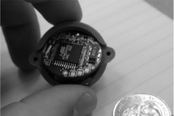
Figure 1-1: DOT – Wireless sensor network device designed to be the approximate size of a
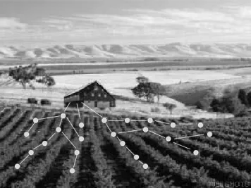
quarter. Future devices will continue to be smaller, cheaper and longer lasting. 2 Figure 1-2: Possible deployment of ac-hoc wireless embedded network for precision
agriculture. Sensors detect temperature, light levels and soil moisture at hundreds of
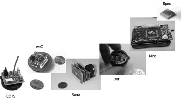
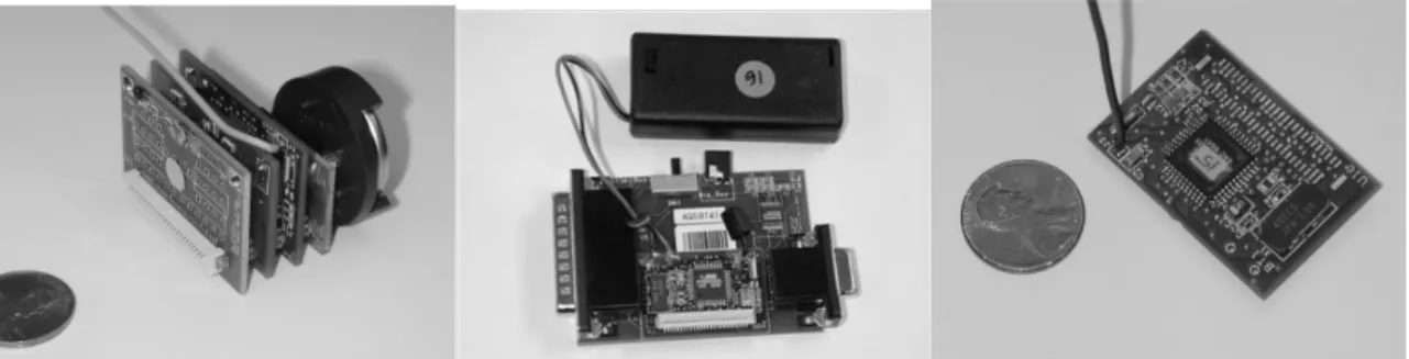
points across a field and communicate their data over a multi-hop network for analysis. 4 Figure 1-3: Design lineage of Mote Technology. COTS (Common off the shelf) prototypes
lead to the weC platform. Rene then evolved to allow sensor expansion and enabled hundreds of compelling applications. The Dot node was architecturally the same as Rene but shrunk into a quarter-sized device. Mica – discussed in depth in this thesis – made significant architectural improvements in order to increase performance and
efficiency. Spec represents the complete integrated CMOS vision. 7
Figure 2-1: Battery characteristics for Lithium, Alkaline and NiMH batteries. The discharge characteristics of alkaline batteries make it essential to design a system to tolerate a
wide range of input voltages. 33
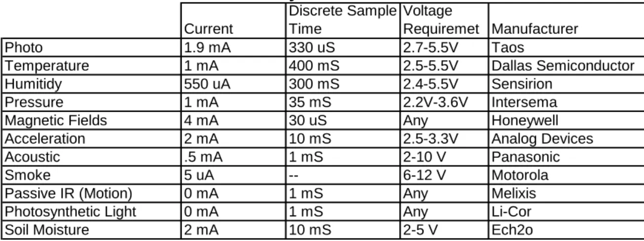
Figure 2-2: Power consumption and capabilities of commonly available. 48
Figure 2-3: Pictures of the Rene wireless sensor network platform. 52
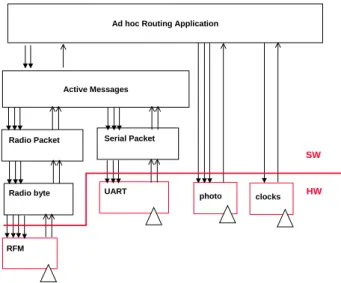
Figure 3-1: Component graph for a multi-hop sensing application. 61
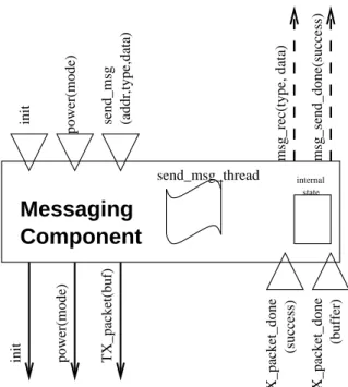
Figure 3-2: AM Messaging component graphical representation. 64
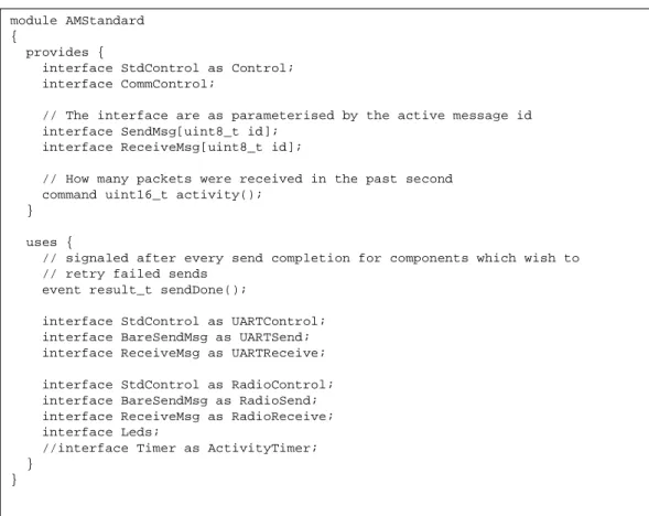
Figure 3-3: NESC component file describing the external interface to the AMStandard
messaging component. 66
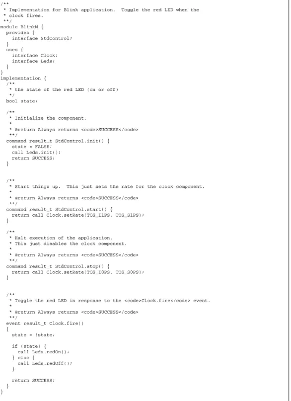
Figure 3-4: BlinkM.nc application component that blinks the system LED's once per second. 68 Figure 3-5: NESC application configuration file that wires together the Blink application. 69 Figure 3-6: Listing of components contained in TinyOS 1.0. Application developers select
from this collection of system-level components to create the desired application
attributes. 77
Figure 3-7: Detailed breakdown of work distribution and energy consumption across each
layer on the Rene node. 80
Figure 4-1: Phases of wireless communication for transmission and reception. 83 Figure 4-2: Energy cost per bit when transmitting at 10Kbps and 50Kbps broken down into
controller and RF energy. 89
Figure 4-3: Generalized Architecture for embedded wireless device. 94
Figure 4-4: Breakdown of CPU usage for start symbol detection overhead broken down into search time, overhead, and CPU time for applications. For the dedicated controller case the breakdown is included with a realistic 10% chip-to-chip overhead estimate and with
a best-case 0% overhead estimate. 98
Figure 5-1: Block diagram of Mica architecture. The direct connection between application controller and transceiver allows the Mica node to be highly flexible to application
demands. Hardware accelerations optionally assist in communication protocols. 104 Figure 5-2: Breakdown of active and idle power consumption for Mica hardware components
at 3V. 105
Figure 5-3: CPU utilization of start symbol detection. Optimizations enabled by the Mica
node significantly increase CPU efficiency. 110
Figure 5-4: Equations for determining the power consumption of a sleeping network. 113 Figure 5-5: Follow-on to the Mica node, blue increase range and reduces power consumption.
Blue nodes have a 4-6x longer battery life over Mica on alkaline batteries. 121 Figure 6-1: The single chip Spec node pictured next to a ballpoint pen. 124
Figure 6-2: Block Diagram of Spec, the single chip wireless mote. 127
Figure 6-3: Design layout for single chip mote. Large central block contains CPU, timers and hardware accelerators. Across the top are 6 memory banks. The ADC is center left.
The radio is in the bottom right corner. 136
Figure 6-4: Area breakdown of digital logic modules included on Spec. Total area of wiring
Figure 6-5: Overview of the performance improvements achieved by the Spec node’s
hardware accelerators. 146
Figure 7-1: Theoretical node energy consumption when performing environmental data monitoring where data is collected every 4 seconds, averaged and transmitted once every 5 minutes. Each node has a maximum of 5 children nodes and one parent node. The table shows results for Rene, Mica, Blue, Spec. The ratio between Rene power consumption and blue power consumption is also shown. The alarm check cost of blue is larger than that of Mica due to the CC1000 having a longer turn-on time. The
Sensing cost of blue is reduced by a low power ADC in the microcontroller. 151 Figure 7-2: 29 palms application. Motes dropped out of an airplane self-assemble onto an
ad-hoc network in order to monitor for vehicle activity at a remote desert location. 154 Figure 7-3: Data filtering performed locally on modes to amplify and extract vehicle signal.
Time stamp assigned to the highest peak of the red activity line. 157
Figure 7-4: Position estimates of each of the sensing node are updated in response to the result
of the linear regression that estimates the passing vehicle’s velocity. 158 Figure 7-5: Picture of z-car tracking application deployment. Remote control car tracked as it
passed through the field of sensors. 160
Figure 7-6: Multi-hip network routing used in z-car tracking application. Nodes detecting the event (in green) transmit data to a single leader that transits a single report packet. The report packet travels across the network (dotted line) until it reaches the base node. The
packet contains the estimate of the evader’s (red) position. 164
Figure 8-1: Characteristics and requirements of commercial embedded real-time operating
Chapter 1:
Introduction
The emerging field of wireless sensor networks combines sensing, computation, and communication into a single tiny device. Through advanced mesh networking protocols, these devices form a sea of connectivity that extends the reach of cyberspace out into the physical world. As water flows to fill every room of a submerged ship, the mesh networking connectivity will seek out and exploit any possible communication path by hopping data from node to node in search of its destination. While the capabilities of any single device are minimal, the composition of hundreds of devices offers radical new technological possibilities.
The power of wireless sensor networks lies in the ability to deploy large numbers of tiny nodes that assemble and configure themselves. Usage scenarios for these devices range from real-time tracking, to monitoring of environmental conditions, to ubiquitous computing environments, to in situ monitoring of the health of structures or equipment. While often referred to as wireless sensor networks, they can also control actuators that extend control from cyberspace into the physical world.
The most straightforward application of wireless sensor network technology is to monitor remote environments for low frequency data trends. For example, a chemical plant could be easily monitored for leaks by hundreds of sensors that automatically form a wireless interconnection network and immediately report the detection of any chemical leaks. Unlike traditional wired systems, deployment costs would be minimal. Instead of having to deploy thousands of feet of wire routed through protective conduit, installers
simply have to place quarter-sized device, such as the one pictured in Figure 1-1, at each sensing point. The network could be incrementally extended by simply adding more devices – no rework or complex configuration. With the devices presented in this thesis, the system would be capable of monitoring for anomalies for several years on a single set of batteries.
In addition to drastically reducing the installation costs, wireless sensor networks have the ability to dynamically adapt to changing environments. Adaptation
mechanisms can respond to changes in network topologies or can cause the network to shift between drastically different modes of operation. For example, the same embedded network performing leak monitoring in a chemical factory might be reconfigured into a network designed to localize the source of a leak and track the diffusion of poisonous gases. The network could then direct workers to the safest path for emergency evacuation.
Current wireless systems only scratch the surface of possibilities emerging from the integration of low-power communication, sensing, energy storage, and computation.
Figure 1-1: DOT – Wireless sensor network device designed to be the approximate size of a quarter. Future devices will continue to be smaller, cheaper and longer lasting.
Generally, when people consider wireless devices they think of items such as cell phones, personal digital assistants, or laptops with 802.11. These items costs hundreds of dollars, target specialized applications, and rely on the pre-deployment of extensive infrastructure support. In contrast, wireless sensor networks use small, low-cost embedded devices for a wide range of applications and do not rely on any pre-existing infrastructure. The vision is that these devise will cost less that $1 by 2005.
Unlike traditional wireless devices, wireless sensor nodes do not need to
communicate directly with the nearest high-power control tower or base station, but only with their local peers. Instead, of relying on a pre-deployed infrastructure, each
individual sensor or actuator becomes part of the overall infrastructure. Peer-to-peer networking protocols provide a mesh-like interconnect to shuttle data between the thousands of tiny embedded devices in a multi-hop fashion. The flexible mesh architectures envisioned dynamically adapt to support introduction of new nodes or expand to cover a larger geographic region. Additionally, the system can automatically adapt to compensate for node failures.
The vision of mesh networking is based on strength in numbers. Unlike cell phone systems that deny service when too many phones are active in a small area, the interconnection of a wireless sensor network only grows stronger as nodes are added. As long as there is sufficient density, a single network of nodes can grow to cover limitless area. With each node having a communication range of 50 meters and costing less that $1 a sensor network that encircled the equator of the earth will cost less that $1M.
An example network is shown in Figure 1-2. It depicts a precision agriculture deployment—an active area of application research. Hundreds of nodes scattered
throughout a field assemble together, establish a routing topology, and transmit data back to a collection point. The application demands for robust, scalable, low-cost and easy to deploy networks are perfectly met by a wireless sensor network. If one of the nodes should fail, a new topology would be selected and the overall network would continue to deliver data. If more nodes are placed in the field, they only create more potential routing opportunities.
There is extensive research in the development of new algorithms for data aggregation [1], ad hoc routing [2-4], and distributed signal processing in the context of wireless sensor networks [5, 6]. As the algorithms and protocols for wireless sensor network are developed, they must be supported by a low-power, efficient and flexible hardware platform.
This thesis focuses on developing the system architecture required to meet the needs of wireless sensor networks. A core design challenge in wireless sensor networks is coping with the harsh resource constraints placed on the individual devices. Embedded
Figure 1-2: Possible deployment of ac-hoc wireless embedded network for precision agriculture. Sensors detect temperature, light levels and soil moisture at hundreds of points across a field and communicate their data over a multi-hop network for analysis.
processors with kilobytes of memory must implement complex, distributed, ad-hoc networking protocols. Many constraints derive from the vision that these devices will be produced in vast quantities and must be small and inexpensive. As Moore’s law marches on, each device will get smaller, not just grow more powerful at a given size. Size reduction is essential in order to allow devices to be produced as inexpensively as possible, as well as to be able to allow devices to be used in a wide range of application scenarios.
The most difficult resource constraint to meet is power consumption. As physical size decreases, so does energy capacity. Underlying energy constraints end up creating computational and storage limitations that lead to a new set of architectural issues. Many devices, such as cell phones and pagers, reduce their power consumption through the use specialized communication hardware in ASICs that provide low-power
implementations of the necessary communication protocols [7] and by relying on high-power infrastructure. However, the strength of wireless sensor networks is their flexibility and universality. The wide range of applications being targeted makes it difficult to develop a single protocol, and in turn, an ASIC, that is efficient for all applications. A wireless sensor network platform must provide support for a suite of application-specific protocols that drastically reduce node size, cost, and power consumption for their target application.
The wireless sensor network architecture we present here includes both a
hardware platform and an operating system designed specifically to address the needs of wireless sensor networks. TinyOS is a component based operating system designed to run in resource constrained wireless devices. It provides highly efficient communication
primitives and fine-grained concurrency mechanisms to application and protocol developers. A key concept in TinyOS is the use of event based programming in conjunction with a highly efficient component model. TinyOS enables system-wide optimization by providing a tight coupling between hardware and software, as well as flexible mechanisms for building application specific modules.
TinyOS has been designed to run on a generalized architecture where a single CPU is shared between application and protocol processing. We detail three generations of wireless nodes and a host of application deployments that have proven the capabilities of our general system architecture. Figure 1-3 lays a picture and timeline of several “mote” generations. The Mica platform has been produced in the largest quantities – over 5000 Mica nodes have been produced and distributed to over 250 companies and research organizations from around the country. The Mica platform includes a low power transceiver, a power management subsystem, extended storage and an embedded microcontroller.
The most advanced hardware platform we present is a single-chip CMOS device that integrates the processing, storage and communication capabilities to form a complete system node. This single chip node – called Spec – measures just 2.5 mm x 2.5 mm, contains a microcontroller, transmitter, ADC, general purpose I/O ports, UART, memory and encryption engine. The tiny chip only needs to be supported by a 32 KHz watch crystal, an off-chip inductor and a power supply, a battery and a 4 MHz clock. The Spec node represents the coming generation of wireless sensor nodes that will be manufactured for pennies and deployed in the millions.
Both the Mica and Spec node are used to substantiate our claim that optimal system architecture for wireless sensor networks is to have a single central controller directly connected to a low-power radio transceiver through a rich interface that supports hardware assistance for communication primitives. In contrast to having a hierarchical partition of hardware resources dedicated to specific functions, a single shared controller performs all processing. This allows for the dynamic allocation of computation
resources to the set of computational tasks demanded by the system. The layers of abstraction typically achieved through hardware partitioning can instead be achieved through the use of a highly efficient software-based component model. Software abstractions allow for a wider scope of cross-layer optimizations that can achieve orders of magnitude improvements is system performance. The power and viability of this architecture is demonstrated through a collection benchmarks performed on real-world hardware and in application level deployments.
Figure 1-3: Design lineage of Mote Technology. COTS (Common off the shelf) prototypes lead to the weC platform. Rene then evolved to allow sensor expansion and enabled hundreds of
compelling applications. The Dot node was architecturally the same as Rene but shrunk into a quarter-sized device. Mica – discussed in depth in this thesis – made significant architectural improvements in order to increase performance and efficiency. Spec represents the complete integrated CMOS vision.
The main contributions of this work are (1) a general architecture that meets the strict efficiency and flexibility requirements of wireless sensor networks, (2) an
implementation of the architecture using current microcontroller and low-power radio technology, (3) an operating system that compliments the hardware capabilities and provides support for sensor network applications, (4) an integrated single chip CMOS hardware platform for use in wireless sensor networks and (5) a demonstration of the flexibility of this architecture on several novel demonstration applications.
This thesis is organized in 9 chapters. Chapter 2 presents three key application scenarios and an overview of the requirements for wireless sensor networks. It is intended to provide the background necessary for a general understanding of the issues discussed in later chapters. Additionally, Chapter 2 provides a general outline of the capabilities of modern hardware building blocks. It culminates in describing a first-generation sensor node used as a baseline for comparison. Chapter 3 presents the overall architecture for the TinyOS operating system and a list of included components. TinyOS is an event based operating system with a highly efficient component model. It plays a critical role in exposing the capabilities of the hardware architectures we present. Chapter 4 discusses the critical design issues that must be addressed by a wireless sensor network platform. We discuss the shortcomings of traditional wireless architectures and present a generalized architecture that addresses these issues. Our generalized
architecture is designed to allow for flexibility without sacrificing efficiency.
In Chapter 5 we present the Mica platform – an off-the-shelf approximation of our generalized architecture. Mica represents what is possible with commercial hardware and allows us to validate the basic principles of our generalized architecture. Mica has
bee successfully used in hundreds of real-world sensor network deployments. Chapter 6 presents the single chip Spec node where communication, computation, and storage are combined onto a 2.5 mm x 2.5 mm die. Spec is a full realization of the generalized architecture presented. Spec represents the future of wireless sensor network hardware. Chapter 7 presets an overview and analysis of several demonstration applications. This analysis underscores the performance impact of the architecture presented. Additionally the applications presented demonstrate the flexibility and validate the platform.
Chapter 8 provides a survey of related work. This includes a summary of research efforts that have been layered on top of the system we present as well as other wireless activities. Chapter 9 summarizes the thesis and concludes with a prediction of future technological trends.
Chapter 2:
Wireless Sensor Networks
The concept of wireless sensor networks is based on a simple equation: Sensing + CPU + Radio = Thousands of potential applications As soon as people understand the capabilities of a wireless sensor network, hundreds of applications spring to mind. It seems like a straightforward combination of modern technology.
However, actually combining sensors, radios, and CPU’s into an effective wireless sensor network requires a detailed understanding of the both capabilities and limitations of each of the underlying hardware components, as well as a detailed
understanding of modern networking technologies and distributed systems theory. Each individual node must be designed to provide the set of primitives necessary to synthesize the interconnected web that will emerge as they are deployed, while meeting strict requirements of size, cost and power consumption. A core challenge is to map the overall system requirements down to individual device capabilities, requirements and actions. To make the wireless sensor network vision a reality, an architecture must be developed that synthesizes the envisioned applications out of the underlying hardware capabilities.
To develop this system architecture we work from the high level application requirements down through the low-level hardware requirements. In this process we first attempt to understand the set of target applications. To limit the number of applications that we must consider, we focus on a set of application classes that we believe are representative of a large fraction of the potential usage scenarios. We use this set of
application classes to explore the system-level requirements that are placed on the overall architecture. From these system-level requirements we can then drill down into the individual node-level requirements. Additionally, we must provide a detailed background into the capabilities of modern hardware.
After we present the raw hardware capabilities, we present a basic wireless sensor node. The Rene node represents a first cut at a system architecture, and is used for comparison against the system architectures presented in later chapters.
2.1 Sensor network application classes
The three application classes we have selected are: environmental data collection, security monitoring, and sensor node tracking. We believe that the majority of wireless sensor network deployments will fall into one of these class templates.
2.1.1 Environmental Data Collection
A canonical environmental data collection application is one where a research scientist wants to collect several sensor readings from a set of points in an environment over a period of time in order to detect trends and interdependencies. This scientist would want to collect data from hundreds of points spread throughout the area and then analyze the data offline [8, 9]. The scientist would be interested in collecting data over several months or years in order to look for long-term and seasonal trends. For the data to be meaningful it would have to be collected at regular intervals and the nodes would remain at known locations.
At the network level, the environmental data collection application is
data back to a set of base stations that store the data using traditional methods. These networks generally require very low data rates and extremely long lifetimes. In typical usage scenario, the nodes will be evenly distributed over an outdoor environment. This distance between adjacent nodes will be minimal yet the distance across the entire network will be significant.
After deployment, the nodes must first discover the topology of the network and estimate optimal routing strategies [10]. The routing strategy can then be used to route data to a central collection points. In environmental monitoring applications, it is not essential that the nodes develop the optimal routing strategies on their own. Instead, it may be possible to calculate the optimal routing topology outside of the network and then communicate the necessary information to the nodes as required. This is possible
because the physical topology of the network is relatively constant. While the time variant nature of RF communication may cause connectivity between two nodes to be intermittent, the overall topology of the network will be relatively stable.
Environmental data collection applications typically use tree-based routing
topologies where each routing tree is rooted at high-capability nodes that sink data. Data is periodically transmitted from child node to parent node up the tree-structure until it reaches the sink. With tree-based data collection each node is responsible for forwarding the data of all its descendants. Nodes with a large number of descendants transmit significantly more data than leaf nodes. These nodes can quickly become energy bottlenecks [11, 12].
Once the network is configured, each node periodically samples its sensors and transmits its data up the routing tree and back to the base station. For many scenarios, the
interval between these transmissions can be on the order of minutes. Typical reporting periods are expected to be between 1 and 15 minutes; while it is possible for networks to have significantly higher reporting rates. The typical environment parameters being monitored, such as temperature, light intensity, and humidity, do not change quickly enough to require higher reporting rates.
In addition to large sample intervals, environmental monitoring applications do not have strict latency requirements. Data samples can be delayed inside the network for moderate periods of time without significantly affecting application performance. In general the data is collected for future analysis, not for real-time operation.
In order to meet lifetime requirements, each communication event must be precisely scheduled. The senor nodes will remain dormant a majority of the time; they will only wake to transmit or receive data. If the precise schedule is not met, the communication events will fail.
As the network ages, it is expected that nodes will fail over time. Periodically the network will have to reconfigure to handle node/link failure or to redistribute network load. Additionally, as the researchers learn more about the environment they study, they may want to go in and insert additional sensing points. In both cases, the
reconfigurations are relatively infrequent and will not represent a significant amount of the overall system energy usage.
The most important characteristics of the environmental monitoring requirements are long lifetime, precise synchronization, low data rates and relatively static topologies. Additionally it is not essential that the data be transmitted in real-time back to the central
collection point. The data transmissions can be delayed inside the network as necessary in order to improve network efficiency.
2.1.2 Security Monitoring
Our second class of sensor network application is security monitoring. Security monitoring networks are composed of nodes that are placed at fixed locations throughout an environment that continually monitor one or more sensors to detect an anomaly. A key difference between security monitoring and environmental monitoring is that security networks are not actually collecting any data. This has a significant impact on the
optimal network architecture. Each node has to frequently check the status of its sensors but it only has to transmit a data report when there is a security violation. The
immediate and reliable communication of alarm messages is the primary system requirement. These are “report by exception” networks.
Additionally, it is essential that it is confirmed that each node is still present and functioning. If a node were to be disabled or fail, it would represent a security violation that should be reported. For security monitoring applications, the network must be configured so that nodes are responsible for confirming the status of each other. One approach is to have each node be assigned to peer that will report if a node is not functioning. The optimal topology of a security monitoring network will look quite different from that of a data collection network.
In a collection tree, each node must transmit the data of all of its decedents. Because of this, it is optimal to have a short, wide tree. In contrast, with a security network the optimal configuration would be to have a linear topology that forms a Hamiltonian cycle of the network. The power consumption of each node is only
proportional to the number of children it has. In a linear network, each node would have only one child. This would evenly distribute the energy consumption of the network.
The accepted norm for security systems today is that each sensor should be checked approximately once per hour. Combined with the ability to evenly distribute the load of checking nodes, the energy cost of performing this check becomes minimal. A majority of the energy consumption in a security network is spent on meeting the strict latency requirements associated with the signaling the alarm when a security violation occurs.
Once detected, a security violation must be communicated to the base station immediately. The latency of the data communication across the network to the base station has a critical impact on application performance. Users demand that alarm situations be reported within seconds of detection. This means that network nodes must be able to respond quickly to requests from their neighbors to forward data.
In security networks reducing the latency of an alarm transmission is significantly more important than reducing the energy cost of the transmissions. This is because alarm events are expected to be rare. In a fire security system alarms would almost never be signaled. In the event that one does occur a significant amount of energy could be dedicated to the transmission. Reducing the transmission latency leads to higher energy consumption because routing nodes must monitor the radio channel more frequently.
In security networks, a vast majority of the energy will be spend on confirming the functionality of neighboring nodes and in being prepared to instantly forward alarm
announcements. Actual data transmission will consume a small fraction of the network energy.
2.1.3 Node tracking scenarios
A third usage scenario commonly discussed for sensor networks is the tracking of a tagged object through a region of space monitored by a sensor network. There are many situations where one would like to track the location of valuable assets or
personnel. Current inventory control systems attempt to track objects by recording the last checkpoint that an object passed through. However, with these systems it is not possible to determine the current location of an object. For example, UPS tracks every shipment by scanning it with a barcode whenever it passes through a routing center. The system breaks down when objects do not flow from checkpoint to checkpoint. In typical work environments it is impractical to expect objects to be continually passed through checkpoints.
With wireless sensor networks, objects can be tracked by simply tagging them with a small sensor node. The sensor node will be tracked as it moves through a field of sensor nodes that are deployed in the environment at known locations. Instead of
sensing environmental data, these nodes will be deployed to sense the RF messages of the nodes attached to various objects. The nodes can be used as active tags that announce the presence of a device. A database can be used to record the location of tracked objects relative to the set of nodes at known locations. With this system, it becomes possible to ask where an object is currently, not simply where it was last scanned [13].
Unlike sensing or security networks, node tracking applications will continually have topology changes as nodes move through the network. While the connectivity
between the nodes at fixed locations will remain relatively stable, the connectivity to mobile nodes will be continually changing. Additionally the set of nodes being tracked will continually change as objects enter and leave the system. It is essential that the network be able to efficiently detect the presence of new nodes that enter the network.
2.1.4 Hybrid networks
In general, complete application scenarios contain aspects of all three categories. For example, in a network designed to track vehicles that pass through it, the network may switch between being an alarm monitoring network and a data collection network. During the long periods of inactivity when no vehicles are present, the network will simply perform an alarm monitoring function. Each node will monitor its sensors waiting to detect a vehicle. Once an alarm event is detected, all or part of the network, will switch into a data collection network and periodically report sensor readings up to a base station that track the vehicles progress. Because of this multi-modal network behavior, it is important to develop a single architecture that and handle all three of these application scenarios.
2.2 System Evaluation Metrics
Now that we have established the set of application scenarios that we are addressing, we explore the evaluation metrics that will be used to evaluate a wireless sensor network. To do this we keep in mind the high-level objectives of the network deployment, the intended usage of the network, and the key advantages of wireless sensor networks over existing technologies. The key evaluation metrics for wireless sensor
networks are lifetime, coverage, cost and ease of deployment, response time, temporal accuracy, security, and effective sample rate. Their importance is discussed below.
One result is that many of these evaluation metrics are interrelated. Often it may be necessary to decrease performance in one metric, such as sample rate, in order to increase another, such as lifetime. Taken together, this set of metrics form a
multidimensional space that can be used to describe the capabilities of a wireless sensor network. The capabilities of a platform are represented by a volume in this
multidimensional space that contains all of the valid operating points. In turn, a specific application deployment is represented by a single point. A system platform can
successfully perform the application if and only if the application requirements point lies inside the capability hyperspace.
One goal of this chapter is to present an understanding of the tradeoffs that link each axis of this space and an understanding of current capabilities. The architectural improvements and optimizations we present in later chapters are then motivated by increasing the ability to deliver these capabilities and increasing the volume of the capability hypercube.
2.2.1 Lifetime
Critical to any wireless sensor network deployment is the expected lifetime. The goal of both the environmental monitoring and security application scenarios is to have nodes placed out in the field, unattended, for months or years.
The primary limiting factor for the lifetime of a sensor network is the energy supply. Each node must be designed to manage its local supply of energy in order to maximize total network lifetime. In many deployments it is not the average node lifetime
that is important, but rather the minimum node lifetime. In the case of wireless security systems, every node must last for multiple years. A single node failure would create a vulnerability in the security systems.
In some situations it may be possible to exploit external power, perhaps by tapping into building power with some or all nodes. However, one of the major benefits to wireless systems is the ease of installation. Requiring power to be supplied externally to all nodes largely negates this advantage. A compromise is to have a handful of special nodes that are wired into the building’s power infrastructure.
In most application scenarios, a majority of the nodes will have to be
self-powered. They will either have to contain enough stored energy to last for years, or they will have to be able to scavenge energy from the environment through devices, such as solar cells or piezoelectric generators [14, 15]. Both of these options demand that that the average energy consumption of the nodes be as low as possible.
The most significant factor in determining lifetime of a given energy supply is radio power consumption. In a wireless sensor node the radio consumes a vast majority of the system energy. This power consumption can be reduced through decreasing the transmission output power or through decreasing the radio duty cycle. Both of these alternatives involve sacrificing other system metrics.
2.2.2 Coverage
Next to lifetime, coverage is the primary evaluation metric for a wireless network. It is always advantageous to have the ability to deploy a network over a larger physical area. This can significantly increase a system’s value to the end user. It is important to keep in mind that the coverage of the network is not equal to the range of the wireless
communication links being used. Multi-hop communication techniques can extend the coverage of the network well beyond the range of the radio technology alone. In theory they have the ability to extend network range indefinitely. However, for a given
transmission range, multi-hop networking protocols increase the power consumption of the nodes, which may decrease the network lifetime. Additionally, they require a minimal node density, which may increase the deployment cost.
Tied to range is a network’s ability to scale to a large number of nodes.
Scalability is a key component of the wireless sensor network value proposition. A user can deploy a small trial network at first and then can continually add sense points to collect more and different information. A user must be confident that the network technology being used is capable of scaling to meet his eventual need. Increasing the number of nodes in the system will impact either the lifetime or effective sample rate. More sensing points will cause more data to be transmitted which will increase the power consumption of the network. This can be offset by sampling less often.
2.2.3 Cost and ease of deployment
A key advantage of wireless sensor networks is their ease of deployment.
Biologists and construction workers installing networks cannot be expected to understand the underlying networking and communication mechanisms at work inside the wireless network. For system deployments to be successful, the wireless sensor network must configure itself. It must be possible for nodes to be placed throughout the environment by an untrained person and have the system simply work.
Ideally, the system would automatically configure itself for any possible physical node placement. However, real systems must place constraints on actual node
placements – it is not possible to have nodes with infinite range. The wireless sensor network must be capable of providing feedback as to when these constraints are violated. The network should be able to assess quality of the network deployment and indicate any potential problems. This translates to requiring that each device be capable of performing link discovery and determining link quality.
In addition to an initial configuration phase, the system must also adapt to
changing environmental conditions. Throughout the lifetime of a deployment, nodes may be relocated or large physical objects may be placed so that they interfere with the
communication between two nodes. The network should be able to automatically reconfigure on demand in order to tolerate these occurrences.
The initial deployment and configuration is only the first step in the network lifecycle. In the long term, the total cost of ownership for a system may have more to do with the maintenance cost than the initial deployment cost. The security application scenario in particular requires that the system be extremely robust. In addition to extensive hardware and software testing prior to deployment, the sensor system must be constructed so that it is capable of performing continual self-maintenance. When necessary, it should also be able to generate requests when external maintenance is required.
In a real deployment, a fraction of the total energy budget must be dedicated to system maintenance and verification. The generation of diagnostic and reconfiguration traffic reduces the network lifetime. It can also decrease the effective sample rate.
2.2.4 Response Time
Particularly in our alarm application scenario, system response time is a critical performance metric. An alarm must be signaled immediately when an intrusion is detected. Despite low power operation, nodes must be capable of having immediate, high-priority messages communicated across the network as quickly as possible. While these events will be infrequent, they may occur at any time without notice. Response time is also critical when environmental monitoring is used to control factory machines and equipment. Many users envision wireless sensor networks as useful tools for industrial process control. These systems would only be practical if response time guarantees could be met.
The ability to have low response time conflicts with many of the techniques used to increase network lifetime. Network lifetime can be increased by having nodes only operate their radios for brief periods of time. If a node only turns on its radio once per minute to transmit and receive data, it would be impossible to meet the application requirements for response time of a security system.
Response time can be improved by including nodes that are powered all the time. These nodes can listen for the alarm messages and forward them down a routing
backbone when necessary. This, however, reduces the ease of deployment for the system.
2.2.5 Temporal Accuracy
In environmental and tracking applications, samples from multiple nodes must be cross-correlated in time in order to determine the nature of phenomenon being measured. The necessary accuracy of this correlation mechanism will depend on the rate of
propagation of the phenomenon being measured. In the case of determining the average temperature of a building, samples must only be correlated to within seconds. However, to determine how a building reacts to a seismic event, millisecond accuracy is required.
To achieve temporal accuracy, a network must be capable of constructing and maintaining a global time base that can be used to chronologically order samples and events. In a distributed system, energy must be expended to maintain this distributed clock. Time synchronization information must be continually communicated between nodes. The frequency of the synchronization messages is dependent on the desired accuracy of the time clock. The bottom line is maintenance of a distributed time base requires both power and bandwidth.
2.2.6 Security
Despite the seemingly harmless nature of simple temperature and light information from an environmental monitoring application, keeping this information secure can be extremely important. Significant patterns of building use and activity can be easily extracted from a trace of temperature and light activity in an office building. In the wrong hands, this information can be exploited to plan a strategic or physical attack on a company. Wireless sensor networks must be capable of keeping the information they are collecting private from eavesdropping.
As we consider security oriented applications, data security becomes even more significant. Not only must the system maintain privacy, it must also be able to
authenticate data communication. It should not be possible to introduce a false alarm message or to replay an old alarm message as a current one. A combination of privacy
and authentication is required to address the needs of all three scenarios. Additionally, it should not be possible to prevent proper operation by interfering with transmitted signals.
Use of encryption and cryptographic authentication costs both power and network bandwidth [16, 17]. Extra computation must be performed to encrypt and decrypt data and extra authentication bits must be transmitted with each packet. This impacts
application performance by decreasing the number of samples than can be extracted from a given network and the expected network lifetime.
2.2.7 Effective Sample Rate
In a data collection network, effective sample rate is a primary application performance metric. We define the effective sample rate as the sample rate that sensor data can be taken at each individual sensor and communicated to a collection point in a data collection network. Fortunately, environmental data collection applications typically only demand sampling rates of 1-2 samples per minute. However, in addition to the sample rate of a single sensor, we must also consider the impact of the multi-hop networking architectures on a nodes ability to effectively relay the data of surrounding nodes.
In a data collection tree, a node must handle the data of all of its descendents. If each child transmits a single sensor reading and a node has a total of 60 descendants, then it will be forced to transmit 60 times as much data. Additionally, it must be capable of receiving those 60 readings in a single sample period. This multiplicative increase in data communication has a significant effect on system requirements. Network bit rates combined with maximum network size end up impacting the effective per-node sample rate of the complete system [5].
One mechanism for increasing the effective sample rate beyond the raw
communication capabilities of the network is to exploit in-network processing. Various forms of spatial and temporal compression can be used to reduce the communication bandwidth required while maintaining the same effective sampling rate. Additionally local storage can be used to collect and store data at a high sample rate for short periods of time. In-network data processing can be used to determine when an “interesting” event has occurred and automatically trigger data storage. The data can then be downloaded over the multi-hop network as bandwidth allows.
Triggering is the simplest form of in-network processing. It is commonly used in security systems. Effectively, each individual sensor is sampled continuously, processed, and only when a security breach has occurred is data transmitted to the base station. If there were no local computation, a continuous stream of redundant sensor readings would have to be transmitted. We show how this same process can be extended to complex detection events.
2.3 Individual node evaluation metrics
Now that we have established the set of metrics that will be used to evaluate the performance of the sensor network as a whole, we can attempt to link the system
performance metrics down to the individual node characteristics that support them. The end goal is to understand how changes to the low-level system architecture impact application performance. Just as application metrics are often interrelated, we will see that an improvement in one node-level evaluation metric (e.g., range) often comes at the expense of another (e.g., power).
2.3.1 Power
To meet the multi-year application requirements individual sensor nodes must be incredibly low-power. Unlike cell phones, with average power consumption measured in hundreds of milliamps and multi-day lifetimes, the average power consumption of wireless sensor network nodes must be measured in micro amps. This ultra-low-power operation can only be achieved by combining both low-power hardware components and low duty-cycle operation techniques.
During active operation, radio communication will constitute a significant fraction of the node’s total energy budget. Algorithms and protocols must be developed to reduce radio activity whenever possible. This can be achieved by using localized computation to reduce the streams of data being generated by sensors and through application specific protocols. For example, events from multiple sensor nodes can be combined together by a local group of nodes before transmitting a single result across the sensor network.
Our discussion on available energy sources will show that a node must consume less that 200 uA on average to last for one year on a pair of AA batteries. In contrast the average power consumption of a cell phone is typically more than 4000 uA, a 20 fold difference.
2.3.2 Flexibility
The wide range of usage scenarios being considered means that the node architecture must be flexible and adaptive. Each application scenario will demand a slightly different mix of lifetime, sample rate, response time and in-network processing. A wireless sensor network architecture must be flexible enough to accommodate a wide
range of application behaviors. Additionally, for cost reasons each device will have only the hardware and software it actually needs for a given the application. The architecture must make it easy to assemble just the right set of software and hardware components. Thus, these devices require an unusual degree of hardware and software modularity while simultaneously maintaining efficiency.
2.3.3 Robustness
In order to support the lifetime requirements demanded, each node must be constructed to be as robust as possible. In a typical deployment, hundreds of nodes will have to work in harmony for years. To achieve this, the system must be constructed so that it can tolerate and adapt to individual node failure. Additionally, each node must be designed to be as robust as possible.
System modularity is a powerful tool that can be used to develop a robust system. By dividing system functionality into isolated sub-pieces, each function can be fully tested in isolation prior to combining them into a complete application. To facilitate this, system components should be as independent as possible and have interfaces that are narrow, in order to prevent unexpected interactions.
In addition to increasing the system’s robustness to node failure, a wireless sensor network must also be robust to external interference. As these networks will often co-exist with other wireless systems, they need the ability to adapt their behavior
accordingly. The robustness of wireless links to external interference can be greatly increased through the use of multi-channel and spread spectrum radios. It is common for facilities to have existing wireless devices that operate on one or more frequencies. The
ability to avoid congested frequencies is essential in order to guarantee a successful deployment.
2.3.4 Security
In order to meet the application level security requirements, the individual nodes must be capable of performing complex encrypting and authentication algorithms. Wireless data communication is easily susceptible to interception. The only way to keep data carried by these networks private and authentic is to encrypt all data transmissions. The CPU must be capable of performing the required cryptographic operations itself or with the help of included cryptographic accelerators [16].
In addition to securing all data transmission, the nodes themselves must secure the data that they contain. While they will not have large amounts of application data stored internally, they will have to store secret encryption keys used in the network. If these keys are revealed, the security of the network could crumble. To provide true security, it must be difficult to extract the encryption keys of from any node.
2.3.5 Communication
A key evaluation metric for any wireless sensor network is its communication rate, power consumption, and range. While we have made the argument that the
coverage of the network is not limited by the transmission range of the individual nodes, the transmission range does have a significant impact on the minimal acceptable node density. If nodes are placed too far apart it may not be possible to create an
interconnected network or one with enough redundancy to maintain a high level of reliability. Most application scenarios have natural node densities that correspond to the
granularity of sensing that is desired. If the radio communications range demands a higher node density, additional nodes must be added to the system in to increase node density to a tolerable level.
The communication rate also has a significant impact on node performance. Higher communication rates translate into the ability to achieve higher effective sampling rates and lower network power consumption. As bit rates increase, transmissions take less time and therefore potentially require less energy. However, an increase in radio bit rate is often accompanied by an increase in radio power consumption. All things being equal, a higher transmission bit rate will result in higher system performance. However, we show later that an increase in the communication bit rate has a significant impact on the power consumption and computational requirement of the node. In total, the benefits of an increase in bit rate can be offset by several other factors.
2.3.6 Computation
The two most computationally intensive operations for a wireless sensor node are the in-network data processing and the management of the low-level wireless
communication protocols. As we discuss later, there are strict real-time requirements associated with both communication and sensing. As data is arriving over the network, the CPU must simultaneously control the radio and record/decode the incoming data. Higher communication rates required faster computation.
The same is true for processing being performed on sensor data. Analog sensors can generate thousands of samples per second. Common sensor processing operations include digital filtering, averaging, threshold detection, correlation and spectral analysis.
It may even be necessary to perform a real-time FFT on incoming data in order to detect a high-level event.
In addition to being able to locally process, refine and discard sensor readings, it can be beneficial to combine data with neighboring sensors before transmission across a network. Just as complex sensor waveforms can be reduced to key events, the results from multiple nodes can be synthesized together. This in-network processing requires additional computational resources.
In our experience, 2-4 MIPS of processing are required to implement the radio communication protocols used in wireless sensor networks. Beyond that, the application data processing can consume an arbitrary amount of computation depending on the calculations being performed.
2.3.7 Time Synchronization
In order to support time correlated sensor readings and low-duty cycle operation of our data collection application scenario, nodes must be able to maintain precise time synchronization with other members of the network. Nodes need to sleep and awake together so that they can periodically communicate. Errors in the timing mechanism will create inefficiencies that result in increased duty cycles.
In distributed systems, clocks drift apart over time due to inaccuracies in timekeeping mechanisms. Depending on temperature, voltage, humidity, time keeping oscillators operate at slightly different frequencies. High-precision synchronization mechanisms must be provided to continually compensate for these inaccuracies.
2.3.8 Size & Cost
The physical size and cost of each individual sensor node has a significant and direct impact on the ease and cost of deployment. Total cost of ownership and initial deployment cost are two key factors that will drive the adoption of wireless sensor
network technologies. In data collection networks, researchers will often be operating off of a fixed budget. Their primary goal will be to collect data from as many locations as possible without exceeding their fixed budget. A reduction in per-node cost will result in the ability to purchase more nodes, deploy a collection network with higher density, and collect more data.
Physical size also impacts the ease of network deployment. Smaller nodes can be placed in more locations and used in more scenarios. In the node tracking scenario, smaller, lower cost nodes will result in the ability to track more objects.
2.4 Hardware Capabilities
Now that we have identified the key characteristics of a wireless sensor node we can look at the capabilities of modern hardware. This allows us to understand what bit rate, power consumption, memory and cost we can expect to achieve. A balance must be maintained between capability, power consumption and size in order to best address application needs. This section gives a quick overview of modern technology and the tradeoffs between different technologies. We start with a background of energy storage technologies and continue through the radio, CPU, and sensors.
2.4.1 Energy
Just as power consumption of system components are often expressed in
milliamps, batteries are generally rated in milliamp-hours (mAh). In theory a 1000 mAh battery could support a processor consuming 10 mA for 100 hours. In practice this in not always true. Due to battery chemistry, voltage and current levels vary depending on how the energy is extracted from a battery. Additionally, as batteries discharge their voltage drops. If the system is not tolerant to a decrease in voltage it may not be possible to use the full rated capacity of a battery. For example, a 1.5 V alkaline battery is not considered empty by the manufacturer until it is outputting only .8 V [18].
2.4.1.1
Battery technologies
There are three common battery technologies that are applicable for wireless sensor networks – Alkaline, Lithium, and Nickel Metal Hydride. An AA Alkaline battery is rated at 1.5 V, but during operation it ranges from 1.65 to .8 V as shown in Figure 2-1 and is rated at 2850 mAh. With a volume of just 8.5 cm3, it has an energy density of approx 1500 Joules/cm3. While providing a cheap, high capacity, energy source, the major drawbacks of alkaline batteries are the wide voltage range that must be tolerated and their large physical size. Additionally, lifetimes beyond 5 years cannot be achieved because of battery self-discharge. The shelf-life of an alkaline battery is approximately 5 years.
Lithium batteries provide an incredibly compact power source. The smallest versions are just a few millimeters across. Additionally, they provide a constant voltage
supply that decays little as the battery is drained. Devices that operate off of lithium batteries do not have to be as tolerant to voltage changes as devices that operate off of alkaline batteries. Additionally, unlike alkaline batteries, lithium batteries are able to operate at temperatures down to -40 C. The most common lithium battery is the CR2032 [19]. It is rated at 3V, 255 mAh and sells for just 16 cents. With a volume of 1 cm3, it has and energy density of 2400 J/cm3. In addition to traditional lithium batteries, there are also specialized Tadiran lithium batteries that have densities as high as 4000 J/cm3 and tolerate a wide temperature range. One of the drawbacks of lithium batteries is that they often have very low nominal discharge currents. A D-cell size Tadiran battery has a
Figure 2-1: Battery characteristics for Lithium, Alkaline and NiMH batteries. The discharge characteristics of alkaline batteries make it essential to design a system to tolerate a wide range of input voltages.
Battery Characteristics
Alkaline discharge curve
Battery Energy Desnsity
0 500 1000 1500 2000 2500 3000 3500 4000 4500 1 J /c m CR2032 Lithium Tadiran Lithium AA Alkaline AA NiMH
nominal discharge current of just 3 mA. This is compared to an alkaline AA battery’s nominal discharge rate of 25 mA.
Nickel Metal Hydride batteries are the third major battery type. They have the benefit of being easily rechargeable. The downside to rechargeable batteries is a
significant decrease in energy density. An AA size NiMH battery has approximately half the energy density of an alkaline battery at approximately 5 times the cost. Before considering the use of NiMH batteries it is important to note that they only produce 1.2 V. Because many system components require 2.7 volts or more, they it may not be possible to operate directly off of rechargeable batteries.
2.4.1.2
Expected lifetime calculation
While it appears easy to quickly look at a battery’s rated capacity, compare it to the systems energy consumption and calculate the system lifetime, there are several additional factors to consider.
In looking at real systems, it is important to look at how power supplies decay over time. Figure 2-1 shows the voltage versus time plot of an AA battery drained at a 500 mW. The graph shows that the battery quickly falls from the 1.5 V starting voltage and ends at just .8 V.
If a theoretical system was built with components requiring 2.7 V and consumed 250 mW, it would only last for 100 minutes off of 2 AA batteries. However, if the system components were selected to operate off of voltages down to 2.0 volts, it would last approximately 5 times as long off of the same power source. A seemingly
2.4.1.3
Voltage Regulation
In order to avoid issues associated with varying battery voltages, voltage
regulation techniques can be used. In general, voltage regulators take in varying input voltages and produce a stable, constant output voltage. Standard regulators require the input voltage be greater than the desired output voltage. Boost converters can output voltages that are higher than the input voltage.
There are two major drawbacks to using voltage regulation. The most obvious is the inefficient conversion process. High efficiency voltage converters can boast of efficiencies up to 90%. However, these are generally tuned for systems consuming hundreds of milliamps. The efficiencies fall drastically as the current consumption of the system is reduced.
Secondly, the quiescent current consumption – or consumption when no current is being output – of regulators can be relatively high. The current consumption of a standard regulator is between 15 and 50 uA. While irrelevant in a system consuming hundreds of milliamps, for ultra-low power devices, this small current drain can dominate overall energy usage.
The inefficiencies associated with voltage conversion and regulation combined with the high variation in output voltage of alkaline batteries makes it highly
advantageous to build sensor nodes out of components that are tolerant to a wide voltage range. Selection of components that can operate over a range of (2.1-3.3V) can
2.4.1.4
Renewable Energy
An alternative to relying on batteries with enough energy to last for years is to use renewable energy. Modern solar cells can produce up to 10 mW per square inch in direct sunlight.