Two Criteria for Model Selection in Multiclass
Support Vector Machines
Lei Wang,
Member, IEEE
, Ping Xue,
Senior Member, IEEE
, and Kap Luk Chan,
Member, IEEE
Abstract—Practical applications call for efficient model selec-tion criteria for multiclass support vector machine (SVM) classification. To solve this problem, this paper develops two model selection criteria bycombining orredefining the radius–margin bound used in binary SVMs. The combination is justified by linking the test error rate of a multiclass SVM with that of a set of binary SVMs. The redefinition, which is relatively heuristic, is in-spired by the conceptual relationship between the radius–margin bound and the class separability measure. Hence, the two criteria are developed from the perspective of model selection rather than a generalization of the radius–margin bound for multiclass SVMs. As demonstrated by extensive experimental study, the minimiza-tion of these two criteria achieves good model selecminimiza-tion on most data sets. Compared with the k-fold cross validation which is often regarded as a benchmark, these two criteria give rise to comparable performance with much less computational overhead, particularly when a large number of model parameters are to be optimized.
Index Terms—Class separability measure, model selection, mul-ticlass classification, mulmul-ticlass support vector machines (SVMs), radius–margin bound.
I. INTRODUCTION
I
N RECENT years, multiclass support vector machines (SVMs) have attracted much attention due to the demands for multicategory classification in many practical applications and the success of SVMs in binary classification. The methods realizing the multiclass SVMs roughly fall into three categories, namely, the methods using the strategies of one-versus-all [1] or one-versus-one [2], [3], the methods based on the error-correcting output codes(ECOC) approach [4], [5], and those using thesingle-machineapproach [6]–[8]. Comparative stud-ies of these methods can be found in [1] and [9]. The one-versus-one- and one-versus-all-based methods are often recommended for practical use because of lower computational cost or conceptual simplicity.Manuscript received February 1, 2007; revised October 31, 2007. First published September 16, 2008; current version published November 20, 2008. This work was supported in part by Nanyang Technological University under Grant LIT 2002-4 of A-STAR and Grant RGM 14/02 and in part by Australian Research Council Discovery Project under Grant DP0773761. The early work of this paper was carried out at Nanyang Technological University, Singapore, Singapore, and the further work of this paper was carried out at The Australian National University, Canberra, A.C.T., Australia. This paper was recommended by Associate Editor S. Singh.
L. Wang is with the Research School of Information Sciences and Engi-neering, The Australian National University, Canberra, A.C.T. 0200, Australia (e-mail: [email protected]).
P. Xue and K. L. Chan are with the School of Electrical and Electronic Engineering, Nanyang Technological University, Singapore 639798 (e-mail: [email protected]; [email protected]).
Digital Object Identifier 10.1109/TSMCB.2008.927272
Similar to binary SVMs, multiclass SVMs also require model selection to achieve good classification performance. Overcom-plex models will overfit training data, whereas oversimple mod-els cannot effectively represent the intrinsic data structure. Both will result in poor classification performance when the classi-fiers are put into use. Just as its binary counterpart, the model selection of multiclass SVMs is used to select the parameters of a kernel function and the regularization parameter that balances training error and machine complexity. Very often, a single model parameter set is uniformly used across all the involved classifiers (for example, the binary SVM classifiers in the one-versus-one- or one-versus-all-based methods), rather than using different parameter sets in different binary classifiers. This is favored because of the following: 1) Much less model parameters need to be determined, particularly when the kernel function has multiple parameters; 2) past studies show little difference on classification performance [10], [11]; and 3) the risk of overfitting is reduced by using a simpler model. Hence, the focus of this paper is on the model selection for multiclass SVMs by finding the best single model parameter set.
In most of the existing work, the model selection for multi-class SVMs uses an exhaustive grid-based search method. The criterion is the k-fold or leave-one-out cross-validation error rate. Although straightforward, the model selection process in this way can become unbearably time consuming because for multiclass SVMs, we are often required to solve larger scale optimization problems. A few methods have been proposed to speed up this process. In [12], generalized approximate cross validation, which is an estimator of the leave-one-out test error rate, is extended to the multiclass setting to tune model parameters. In [13], an error bound for a multiclass SVM using the ECOC approach is developed and applied to the model selection. The grid search is still needed to find the best param-eter set. These methods soon become intractable when three or more model parameters are to be tuned. A genetic algorithm has been used to search the model parameter space for model selection [14], [15]. Again, the selection process becomes very slow when the number of model parameters is large.
Practical applications of multiclass SVMs call for efficient model selection criteria, which should be able to handle more model parameters without leading to unacceptable computation cost. In recent years, model selection for binary SVMs has been well studied, and many selection criteria and methods have been developed [16]–[18]. Our proposed approach in this paper is to develop new criteria based on the principles of the successful criteria in binary SVMs for the multiclass setting. In the model selection for binary SVMs, a class of methods use nonlinear optimization techniques to maximize or minimize a certain
criterion to obtain an optimal model parameter set [19], [20]. They can achieve much more efficient model selection than the straightforward grid search. A significant progress along this direction is the method of minimizing the radius–margin bound of a binary SVM classifier [16], [21]. Chapelle et al.
determine the derivatives of this bound with respect to model parameters, making iterative gradient-based optimization tech-niques applicable. The optimal model parameter set can be efficiently found after a number of iterations. This method not only significantly shortens the model selection process but can also optimize multiple model parameters simultaneously. It is much desired if such a criterion could also be extended to the multiclass setting. However, such a theoretical generalization of this bound is not that straightforward because this bound is rooted in the theoretical basis of binary SVMs. In [22], a theoretical generalization of this bound was reported but without further experimental investigation.
Although an error bound can certainly be used as a model selection criterion, it is unnecessary for a model selection criterion to be a valid error bound. As pointed out in [16], when model selection is of concern, whether the minimum (or maximum) of a criterion aligns well with lower test error rates is more important. Hence, instead of aiming to derive an error bound for a multiclass SVM, our paper focuses on developing practical and efficient model selection criteria by observing the principle of such criteria in a binary setting. In detail, the radius–margin bound for binary SVMs is exploited in the fol-lowing two ways: 1) by linking the test error rates from binary and multiclass SVM classifiers, the first criterion is developed based on the pairwise combination of the radius–margin bounds of a set of binary SVMs for model selection; and 2) inspired by the relationship between the radius–margin bound and the class separability measure, the second criterion defines a new radius and margin to accommodate multiple classes. As shown later, both criteria inherit the elegant properties of the orig-inal radius–margin bound. Their derivatives with respect to model parameters can also be analytically computed, and thus, gradient-based optimization techniques are still applicable. The two criteria allow for efficient optimization for several hundreds of model parameters simultaneously. As before, the optimized kernel parameters can be used to identify more discrimina-tive features, which can be used to perform feature selec-tion in a multiclass scenario. To evaluate the model selecselec-tion performance of the two criteria, extensive experiments were conducted on a variety of benchmark data sets with different numbers of model parameters. Although the two criteria are developed for a multiclass SVM classifier using the one-versus-one classification strategy, the model parameters selected by them are also tested on the classifiers using other classification strategies, including the one-versus-all, ECOC, and the single-machine approach. The experimental results demonstrate the simplicity, effectiveness, and efficiency of the two criteria for model selection in multiclass SVMs.
The rest of this paper is organized as follows. In Section II, the radius–margin bound is briefly introduced. To stay in focus, the details of binary and multiclass SVMs are omitted, and readers are referred to the papers cited earlier. Sections III and IV present the two model selection criteria in detail. In
Section V, computational issue is discussed. Section VI presents experimental results, and the concluding remarks are drawn in Section VII.
II. RADIUS-MARGINBOUND FORBINARYSVMS
Let D denote a set of l training samples and D=
{(x1, y1), . . . ,(xl, yl)} ∈(Rd× Y)l, where Rd denotes a
d-dimensional input space, Y denotes the label set of x, and
y is {±1} in binary classification. A kernel is defined as
kθ(xi,xj) =φ(xi), φ(xj), where φ(·)is a possibly nonlin-ear mapping fromRdto a feature spaceF, andθdenotes the kernel parameter set. For nonseparable data, a regularization parameterCwill be used, and the model parameter set becomes
{θ, C}.
Let L(D) be the number of errors in a leave-one-out pro-cedure performed onD. The radius–margin bound is an upper bound ofL(D). For a hard margin binary SVM, it is shown in [16] that L(D)≤ 4R 2 γ2 = 4R 2w2 (1)
where R is the radius of the smallest sphere enclosing the
l training samples in F, γ is the margin, w is the normal vector of the optimal separating hyperplane, andγ= 1/w. For nonseparable data, an L2-norm soft margin SVM will be used, and the aforementioned result still holds. This is because an L2-norm soft margin can be shown as a hard margin with a slightly modified kernel function k(xi,xj) [16], [23]. The relationship betweenkandkisk(xi,xj) =k(xi,xj) + (1/C) if i=j andk(xi,xj) =k(xi,xj)otherwise, whereC is the regularization parameter mentioned earlier. This is also adopted in this paper. The squared radius R2 is expressed as R2=
minφ(x
i)−ˆc2≤Rˆ2( ˆR
2), whereφ(x
i) (i= 1, . . . , l)is the image ofxiinF,Rˆis the radius of a sphere enclosing all theφ(xi), and ˆc is the center of this sphere. This leads to a quadratic optimization problem, and it can be obtained that
R2= max β∈Rl ⎡ ⎣l i=1 βik(xi,xi)− l i,j=1 βiβjk(xi,xj) ⎤ ⎦ subject to: l i=1 βi = 1; βi≥0 (i= 1,2, . . . , l) (2) where βi is theith Lagrange multiplier and the center of the sphere is represented asˆc=li=1βiφ(xi). As forw2, it can be obtained once the SVM optimization problem is solved. In detail 1 2w 2= max α∈Rl ⎡ ⎣l i=1αi− 1 2 l i,j=1 αiαjyiyjk(xi,xj) ⎤ ⎦ subject to: l i=1 αiyi= 0; αi≥0 (i= 1,2, . . . , l) (3) whereαiis theith Lagrange multiplier. The derivatives ofR2 and w2 with respect to the model parameters are given in
[16]. Letθt(θt∈θ)be thetth model parameter ∂R2 ∂θt = l i=1 βi∂k(xi,xi) ∂θt − l i,j=1 βiβj∂k(xi,xj) ∂θt (4)
whereβi(i= 1,2, . . . , l)is the solution of (2). The derivative ofw2with respect toθ tis given as ∂w2 ∂θt = (−1)· l i,j=1 αiαjyiyj ∂k(xi,xj) ∂θt (5)
whereαi(i= 1,2, . . . , l)is the solution of (3). This way, the derivative of the radius–margin bound with respect toθtis
∂ R2w2 ∂θt =w2∂R 2 ∂θt +R2∂w 2 ∂θt . (6)
The model selection with the radius–margin bound is briefly described as follows.
1) Setθrto an initial valueθ0.
2) Based on the currentθr, optimize forαandβbased on (3) and (2), respectively, and denote the optimal solutions byα
randβr. 3) Onceα
r andβr are obtained, the derivative in (6) can be explicitly computed for a givenθr. Thus, a gradient-based search method can be used to minimize R2w2
with respect toθr. The minimizer is denoted byθr+1. 4) Stop if a given stopping criterion is satisfied andθr+1is
the selected model. Otherwise, letθr←−θr+1and go to Step 2).
As demonstrated, the radius–margin bound is rooted in the theoretical basis of binary SVMs, and it cannot be directly used in model selection for multiclass SVMs. In the rest of this paper, two criteria are developed based on this bound to deal with model selection in multiclass SVMs.
III. MODELSELECTIONCRITERIONI
Let D and Dt denote the training and test data sets, re-spectively.E(Dt)denotes the number of misclassified samples obtained by applying a multiclass SVM classifier toDt. The classifier and the test set are assumed to be fixed but unknown. For ac-class problem
E(Dt) = c i=1 c j=1,j=i Eij(Dt). (7)
Eij(Dt) denotes the number of samples misclassified from classito classj,1and it is expressed as
Eij(Dt) =x|x∈ Dt, y0(x) =i, ym(x) =j (8)
1Without loss of generality, the cost of misclassification is considered as identical among the classes in (7). The case having different misclassification costs will be discussed at the end of Section IV.
where | · | denotes the size of a set.2 A sample x inD t will be counted into Eij(Dt)if and only if its true label y0 is i, whereas the labelympredicted by a multiclass SVM classifier isj. Considering that both true and predicted labels are unique for each sample,3 a misclassified sample will not be counted into two differentEij’s. Hence, there is no overlapping among theseEij’s.
Let us focus on the one-versus-one strategy with the max winsclassification rule [9]. It is commonly used to solve mul-ticlass SVM problems. With this strategy, a set of c(c−1)/2
pairwise binary SVM classifiers are constructed. Let SVMij denote the binary SVM classifier trained with the samples from classes i and j. The Eij(Dt) is the number of test samples which belong to class ibut are misclassified to class j when SVMij is applied to classesi and j. For the convenience of notation, the label predicted by SVMij is written as i or j although it is +1 or −1 in general. TheEij (Dt) is formally expressed as
Eij (Dt) =x|x∈ Dt, y0(x) =i, ybij(x) =j (9) whereyb
ij(x)stands for the label predicted by the binary SVM classifier, SVMij. The total number of errors made by thec(c−
1)/2binary SVM classifiers is
E(Dt) =
1≤i,j≤c,i=j
Eij (Dt). (10)
The following proves that E(Dt) is upper bounded by
E(Dt). Under the rule of max wins [9], the label of a test samplexis decided by
ym(x) = arg max
i=1,...,cSi(x) = arg maxi=1,...,c
⎛ ⎝ c j=1,j=i sign[wij, φ(x)+bij] ⎞ ⎠ (11) wherewij, φ(x)+bij is positive ifxis classified to classi. The sign(a)denotes the sign function, and it is+1 fora >0,0
fora= 0, and−1 otherwise. The summation over the(c−1)
sign functions is a score, and it is denoted bySi(x)for classi. The samplexis assigned to the class having the highest score. This rule immediately leads to the following three results.
1) ∀x∈ Dt, there must be Si(x)≤(c−1)(i= 1, . . . , c), and the equality is achieved if and only if all the (c−
1) binary SVM classifiers SVMij (j= 1, . . . , c, j=i) classifyxto classi.
2) IfSi(x)< Sj(x), there must beSi(x)<(c−1). Refer-ring to result 1), this indicates that at least one of the
(c−1) binary SVM classifiers does not classify x to classi.
2Please note that according to the definition ofDt, “x∈ Dt” in (8) should be written as “(x, y0(x))∈ Dt.” However, the former is used in this paper for the convenience of notation.
3In multilabel classification, the true and predicted labels may not be unique for a sample. This paper confines itself to multiclass problems.
3) IfSi(x) =Sj(x), then both of them must be smaller than
(c−1). This is because the binary SVMijcannot classify
xto both classesiandjsimultaneously.
Assume that a multiclass SVM misclassifies a test sample
xt(xt∈ Dt). That is, the true label y0(xt) is i, whereas the predicted label ym(x
t) is j. This contributes one count to
Eij(Dt) based on (8). By referring to (11), this means that
Sj(xt) is the highest score, and hence, Si(xt)≤Sj(xt). By applying results 2) and 3), it is obtained thatSi(xt)<(c−1), indicating that at least one of the(c−1)binary SVMs has mis-classified the samplext. This contributes one count toEik (Dt); however, please note thatkis not necessary to be exactly thej inEij(Dt). Therefore, for any test sample misclassified by a multiclass SVM, it must have been misclassified by at least one binary SVM classifier. SummingEij andEik overiandj(or
k) gives rise to 1≤i,j≤c,i=j Eij≤ 1≤i,k≤c,i=k Eik ⇐⇒E(Dt)≤E(Dt). (12) This proves thatE(Dt)is upper bounded by E(Dt). Mean-while, it is worth mentioning that Eij(Dt)≤Eij (Dt) is not necessary to be true.
The aforementioned result suggests that to reduce the value ofE(Dt), we could seek to minimize its upper boundE(Dt). This leads to one model selection criterion as follows. As known from (1) in Section II, the test error (Eij +Eji) can be estimated through the leave-one-out error of SVMij, which is denoted byLij, that satisfies
Lij ≤4R2ijwij2. (13) Thus, the E(Dt) can be estimated by
1≤i<j≤cLij, and it satisfies 1≤i<j≤c Lij ≤ 1≤i<j≤c 4R2ijwij2. (14) To minimizeE(Dt)(or more precisely, to minimize its esti-mate), the right side has to be minimized.
Based on the aforementioned analysis, the
1≤i<j≤cR2ijwij2is defined as a model selection criterion for multiclass SVMs. It is a pairwise combination of the radius–margin bounds of the binary SVM classifiers. The optimal model parameter set is obtained by
θ∗= arg min θ∈Θ ⎛ ⎝ 1≤i<j≤c Rij2wij2 ⎞ ⎠. (15)
The derivative of this criterion with respect to thetth model parameterθtis ∂ ∂θt ⎛ ⎝ 1≤i<j≤c R2ijwij2 ⎞ ⎠ = 1≤i<j≤c wij2 ∂R2 ij ∂θt +R2ij∂wij 2 ∂θt . (16) The calculation of∂R2
ij/∂θtand∂wij2/∂θtfollows (4) and (5). As in a binary classification, the optimal model parameter set θ∗ can be found by using gradient-based optimization techniques.
Before ending this section, it is interesting to look into the relationship between the proposed model selection criterion and the radius–margin bound generalized for multiclass SVMs in [22]. In that work, the multiclass SVM is solved by the
single-machineapproach. With the notations in this paper, the generalized bound in [22] can be expressed as
L(D)≤(4K/c) ⎛ ⎝R2 1≤i<j≤c wi−wj2 ⎞ ⎠ (4K/c) ⎛ ⎝R2 1≤i<j≤c wij2 ⎞ ⎠ (17) whereKis a constant andcis the number of classes. In [22],R
denotes the radius of the smallest sphere enclosing the support vectors only. In this paper, R is changed to enclose all the training samples. Note that such a change will not affect the “≤” in (17) because the newRis an upper bound of the original one. The work in [22] adopts the multiclass SVMs proposed by [6]. There, the(wi−wj)can be understood as awij, which is a normal vector of an SVM hyperplane separating classesi
andj. For the proposed Criterion I in (15),Rij is the radius of the smallest sphere enclosing the training samples from classes
iandj, and therefore,R2
ij≤R2. Replacing allR2ijin (15) with
R2and movingR2 out of the summation sign turn Criterion I to(R2
1≤i<j≤cwij2). If the constant(4K/c)is ignored, the proposed Criterion I and the generalized bound in [22] will share similar structures. Surely, from the perspective of generalizing a bound in a strict theoretical sense, the approach in [22] is more suitable.
IV. MODELSELECTIONCRITERIONII
Class separability is a concept widely used in pattern recog-nition [24]–[26]. The scatter-matrix-based measure is often favored, thanks to its simplicity and applicability to both binary and multiclass problems. They are defined as
SW = c i=1 x∈Di (x−mi)(x−mi) SB= c i=1 ni(mi−m)(mi−m) ST = c i=1 x∈Di (x−m)(x−m) =SW +SB. (18)
cis the number of classes,Diis the set of training samples from class i, andni is the size of Di.mi andm are the class and total means, respectively. Many combinations of two of SW,
SB, and ST can be used as a class separability measure. The commonly used ones includetr(SB)/tr(SW)and|SB|/|SW|,
where tr(A) and |A| denote the trace and determinant of a square matrixA, respectively. Other combinations can be found in [26].
In our previous work [27], we restrict to binary classification and preliminarily discuss the relationship between the scatter-matrix-based class separability measure and the radius–margin bound. Now, this discussion is extended to a multiclass case and is used to develop the second model selection criterion. To do so, the following first extends the class separability to a kernel-induced feature space F. Considering that the high dimensionality ofF can easily make the scatter matrices sin-gular and their determinants zero, the trace-based measure is used instead. In the following, the superscript φ is used to distinguish the variables inFfrom those inRd. Recall thatD
i denotes the training samples from theith class.Dis defined as the union of Di (i= 1,2, . . . , c), which is expressed as D=
∪c
i=1Di.KA,Bis a kernel matrix where{KA,B}ij =k(xi,xj), with the constraints of xi∈ A and xj∈ B. Sum(·) denotes the summation of all the elements in a matrix. The traces are obtained as tr SφB = c i=1 Sum(KDi,Di) ni − Sum(KD,D) n (19) tr SφW = tr(KD,D)− c i=1 Sum(KDi,Di) ni (20) tr SφT = tr(KD,D)−Sum(nKD,D). (21)
To facilitate analysis, the class separability measure in F is defined as tr(SφB)/tr(SφT) instead of tr(SφB)/tr(SφW). Note that they are essentially identical becausetr(SφT) = tr(SφB) + tr(SφW).
Recall thatn1 andn2 are the sizes of D1 andD2, respec-tively. The relationship betweentr(SφB)and the squared margin
γ2can be proven as (the proof is omitted)
γ2≤ 1 4− n1+n2 n1n2 tr SφB = 1 4−mφ1−mφ22 . (22)
This result indicates that 1/(4− mφ1−mφ22) is an upper bound ofγ2. The equality in “≤” is achieved if and only if the solution of the problem in (3), denoted by αi, is 1/n1 for xi∈ D1 and 1/n2 for xi∈ D2. Considering that such a solution seldom occurs in practice,1/(4− mφ1−mφ22) is a strict upper bound in general. Recall that when minimizing the radius–margin bound for the model selection,γ2 is to be maximized. Based on (22), to allowγ2 to be maximized, its upper bound needs to be adequately large, and it will preventγ2 from being increased otherwise. This, in turn, requiresmφ1 −
mφ22to be adequately large. Meanwhile, decreasing the value ofmφ1−mφ22will reduce the upper bound value, forcingγ2
to be kept small. Please note that although a larger (or smaller)
mφ1 −mφ22does not necessarily lead to a larger (or smaller)
γ2, their values are often strongly positively correlated to each other in practice, which can be seen from the results comparing the values of−tr(SφB)andw2in our previous work [27].
A similar result can be proven for the squared radiusR2as
R2≥ 1 (n1+n2) tr SφT . (23)
It shows that tr(SφT)/(n1+n2) is a lower bound of
R2. The equality in “≥” is achieved if and only if the solution of the problem in (2), denoted byβi, is1/(n1+
n2)for all the training samples. Again, such a solution is rare in practice, and this is a strict lower bound in general. When minimizing the radius–margin bound for the model selection,
R2 is to be minimized. Based on (23), this needs tr(Sφ T) to be adequately small to avoid hindering the decrease ofR2. In addition, it can be seen from [27] that the values oftr(SφT)and
R2are often strongly positively correlated.
Conceptually speaking, mφ1−mφ22 and γ2 reflect the similar property of data separation, whereas tr(SφT) and R2 measure the similar property of data scattering. Inspired by the aforementioned results, this paper transplants the radius–margin bound to a multiclass scenario by mimicking the class separability measure. At the same time, please note that this new model selection criterion will still be based onRand
wrather than the traces of the scatter matrices.
In a multiclass case,tr(SφT)/(n1+n2)measures the average of the squared scattering radius of the training samples in F. Considering the analogy betweentr(SφT)/(n1+n2)andR2in a binary classification, the new criterion redefines R2 as the radius of the smallest sphere enclosingallthe training samples from thecclasses
R2c = min
φ(x)−ˆc2≤Rˆ2
( ˆR2) ∀x∈ D. (24)
Fortr(SφB), it can be shown that in the case ofcclasses
tr SφB = 1≤i<j≤cninjmφi −m φ j 2 n2 . (25)
By noting the analogy between mφ1−mφ22 and γ2 in a binary classification, the margin in the new criterion is re-defined as γ2= 1≤i<j≤cninjγ2ij n2 = 1≤i<j≤c PiPjwij−2 (26) where γij is the margin of the binary SVM classifier trained with the training samples of classes i andj, andPi=ni/n, which is the prior probability of class i estimated from the training samples. The redefined margin is a weighted average of those from the pairwise binary SVM classifiers, and the weight is the product of the prior probabilities of the two involved classes. This implies that the margins between the classes dominating the training and test sets need to be emphasized. Otherwise, the number of misclassified samples will be high. This agrees with the intuition. In this way, the second model
TABLE I
COMPARISON OFCOMPUTATIONALLOAD
selection criterion is obtained, and the optimal model parameter set is given by θ∗= arg min θ∈Θ R2 c γ2 . (27)
The derivative of this criterion with respect to thetth model parameterθtis ∂ ∂θt R2 c γ2 = 1 γ4 γ2∂R 2 c ∂θt − R2c∂γ 2 ∂θt (28) where ∂γ2 ∂θt =− ⎛ ⎝ 1≤i<j≤c PiPjwij−4 ∂wij2 ∂θt ⎞ ⎠. (29) Again, the minimization of this bound can be achieved by using the gradient-based optimization techniques. Compared with Criterion I, this criterion is more heuristic and is farther from being interpreted as a bound of generalization error.
Finally, please note that these two criteria can be conve-niently extended to handle the case where the misclassification costs between different classes are different. The first crite-rion is currently a pairwise combination of the radius–margin bounds with equal weights. When different misclassification costs are defined, a weighted combination can be applied in-stead. A larger weight will be assigned if the misclassification cost among a certain pair of classes is higher. For the second criterion, the weighting can be applied to the pairwise combi-nation of margins. In the terminology of class separability, this means that two classes with higher misclassification cost will be pushed farther away from each other to reduce the potential misclassification chances.
V. COMPUTATIONALISSUE
Both criteria have continuous first- and second-order deriv-atives with respect to the model parameters as long as the employed kernel function has. The minimization of them can be efficiently solved by using gradient-based optimization tech-niques. For example, the Broyden–Fletcher–Goldfarb–Shanno (BFGS) quasi-Newton method [28] is often favored because it commonly takes a smaller number of iterations before conver-gence. At each iteration, the computational load is largely due to the evaluation of the objective function. LetQP(n)denote a quadratic programming problem with n training samples. Letsbe the number of values tried for each model parameter
in an exhaustive grid-based search method.|θ| is the number of model parameters to be optimized, and k is the number of folds of cross validation. Besides these, e stands for the number of function evaluations in an optimization process. The computational loads of the model selection methods reviewed in Section I are listed in Table I. Following [16], the measure in terms ofthe total number of QP problems to be solvedis used.4 As shown in Table I, for a multiclass SVM classifier using the one-versus-all strategy, training this classifier results in the computational cost ofc·QP(n). For that using the one-versus-one strategy, this result becomes1≤i<j≤cQP(ni+nj). Cal-culating R2
c and R2ij (or wij2) in the proposed criteria involves oneQP(n)and oneQP(ni+nj), respectively. From this table, it is found that the computational load of grid-based search methods increases rapidly with the increasing value of
s,|θ|, ork. They quickly become intractable when|θ|is larger than three. In contrast, the proposed criteria have a much lower computational load, thanks to the applicability of gradient-based optimization techniques. As shown in the experimental study, the minimization of them can be accomplished in a few iterations with a number of function evaluations, even if|θ|is as large as several hundreds. Compared with the existing methods, the proposed criteria can save considerable computational cost, and the more the model parameters, the more the savings will be.
VI. EXPERIMENTALRESULT
This experiment evaluates the effectiveness of the proposed criteria for the model selection of multiclass SVMs. Two forms of the Gaussian radial basis function (GRBF) ker-nel are used. One is the spherical GRBF kernel k(x,y) = exp(−(x−y2/2σ2)), where σ is the kernel parameter known as the Gaussian width. In this case, the model param-eter set is θ={C, σ}, and C is the regularization parameter. The other is theellipsoidalGRBF kernel that assigns different
σ’s to each feature dimension. It is expressed as k(x,y) = exp(−di=1((xi−yi)2/2σ2i)), where σi is the Gaussian width for the ith dimension. At this time, θ expands to
{C, σ1, σ2, . . . , σd}. In this experiment, the two kernels are used to evaluate the performance of the proposed criteria in
4The computational load is also affected by the dimensionality of data and the computation of a kernel function. They are considered as constants for a given multiclass SVM classification problem.
TABLE II
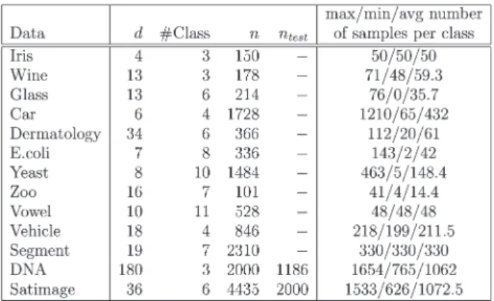
ATTRIBUTES OF THEMULTICLASSBENCHMARKDATASETS
dealing with small- and large-sized model parameter sets, re-spectively.
The BFGS quasi-Newton method is employed to minimize the two criteria to find the optimal model parameter set. To avoid the constraints ofC >0 and σ >0, the transforms of
μ=−ln(C) and ν= ln(g) = ln(1/2σ2) are applied, where
ln(·)denotes the natural logarithm.μandν(orν1, . . . , νdwhen an ellipsoidal GRBF kernel is used) are optimized instead. Thus, the minimization of the criteria becomes an uncon-strained optimization problem. The initial values of μ andν
are set asμ0= 0(or, equally, C= 1) andν0=−ln(2d)(or, equally, σ=√d), where d is the dimension of the feature vector. Note that for a data set, the feature components along each dimension have been linearly scaled to [−1, +1] by using the training samples. The feature components of the test samples will be scaled with the same scaling parameters when doing classification.
Following the work in [21], two stop criteria are used, and the optimization will terminate when either of them is satisfied. Letθt andθt+1denote the model parameters obtained in the
tth and (t+ 1)th iterations, respectively. f(θt) andf(θt+1) are the corresponding values of the objective function. The first stop criterion is|f(θt+1)−f(θt)| ≤f(θt), whereis a small positive number which is set as10−5in this experiment. With this stop criterion, the optimization will terminate if the difference of the function values in two consecutive iterations is less than a predefined tolerance. The second stop criterion is specifically designed for the minimization of the radius–margin bound in [21]. At each iteration of the BFGS quasi-Newton algorithm, a line search is carried out to find the starting point and direction for the next iteration. However, as pointed out in [21], too many line searches may be conducted at a single iteration when the minimum of the bound is being approached. The reason is that in practice, the derivatives computed based on (4) and (5) may slightly deviate from their theoretical values. When the minimum of the bound is being approached, the derivatives will be small, and the impact of this deviation will become significant. Due to the inaccurate derivative information, an iteration may take many line searches to find a solution. To deal with this, the second stop criterion terminates the optimization if the number of line searches at an iteration exceeds a predefined value, for example, ten.
Benchmark data sets fromUCIMachine Learning Repos-itory and Statlog Project are used, and they are listed in Table II.ddenotes the dimensionality, “#Class” is the number of classes, and n is the size of a data set. For “DNA” and “Satimage,” n and ntest are the sizes of the training and test sets, respectively. The last column in Table II lists the maximum, minimum, and average numbers of samples in each class. Following the work in [16] and [29], for a data set without predefined training/test sets, the whole data set is randomly split as 100 pairs of training/test subsets (50%:50%), and the first five training subsets are used for model selection. For “DNA” and “Satimage,” the predefined training sets are randomly split as five pairs of training/test subsets, and the five training subsets are used for the model selection. This experiment uses a mixture of codes inCandMatlab. TheC version of LIBSVM [30] is used to optimize R2 andw2, as well as in training and testing an SVM classifier. The BFGS quasi-Newton algorithm is realized by using the Matlab functionfminunc().
There are three parts in this experiment. First, the properties of the proposed two criteria are demonstrated. Second, their effectiveness for multiclass SVM model selection is evaluated on the benchmark data sets. Finally, its application to feature selection is briefly demonstrated through a toy problem and an optical digit recognition task.
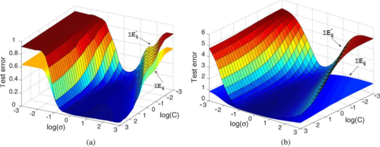
A. Properties of the Two Model Selection Criteria 1) Relation Between Eij,
Eij , and Criterion I: As defined earlier,Eij is the number of test samples misclassified from classitoj when a multiclass SVM classifier is applied, whereas Eij is such a number when a binary SVM classifier SVMij is used. In this paper, the minimization of
Eij is sought by minimizing its upper bound Eij , and this gives rise to Criterion I. In this experiment, with different pairs of
Candσ, the values ofEij,
Eij , and Criterion I are cal-culated and compared. The results on the “Wine” and “Vowel” data sets are shown in Fig. 1. The axes areln(C),ln(σ), and test error, respectively. The curved surfaces of Eij and
Eij
are labeled by arrows. It can be seen from both subfigures that the two surfaces show similar profiles with respect to ln(C)
and ln(σ), although their magnitudes are different when the test error is large. To quantitatively measure the correlation between them, Eij and
Eij are treated as two random variables. The correlation coefficientρis calculated and listed under each subfigure. The two variables are found to be strongly positively correlated, indicating that a smallerEij generally corresponds to a smaller Eij. Similar results are also ob-served from other data sets. These results preliminarily show that it is sensible to useEij to estimateEijfor the model selection.
Now, the correspondence between the test errorEij and Criterion I is further checked. The Eij and the criterion values often do not have such a strong correlation as Eij andEij do. This is because the radius–margin bound is not a tight bound of test error in a binary classification [16]. Fig. 2 shows their correspondence on the data set of “Vowel.” Fig. 2(a) and (b) show the values ofEijand Criterion I, respectively. This is a top view, and the color bar on the right side indicates
Fig. 1. Correspondence betweenEij andEij(ρis the correlation coefficient between them). (a) Wine,ρ= 0.998. (b) Vowel,ρ= 0.942.
Fig. 2. Correspondence betweenEijand Criterion I. (a) Vowel,
Eij. (b) Vowel, Criterion I.
the magnitude. Eij and Criterion I show similar contours, and the region of smaller criterion values aligns well with that of lower test error rates. Similar results are also seen from other data sets. These observations suggest that it is possible to locate the region of lower test error rates by minimizing Criterion I. This will be further verified later by more experimental study. On the other hand, one exceptional case is also found on the data set of “Vehicle.” There, the region of lower criterion values does not align with the area of lower test error rates. Further investigation finds that the radius–margin bound on classes 1 and 2 is too loose to reasonably reflect the value of
(E12 +E21 ).
2) Relationship Between the Class Separability Measure and Criterion II: As mentioned before, there is some relationship between the scatter-matrix-based class separability measure and the radius–margin bound. Inspired by this, Criterion II is developed. Although this relationship is not directly related to the efficiency of this criterion, it is still demonstrated in this experiment for the sake of integrity. After this, the cor-respondence between Eij and Criterion II will be shown. Fig. 3 shows the class separability and the radius–margin bound calculated by using the first two classes of the “Wine” data set. The results are shown in Fig. 3(a) and (b), respec-tively. Along the axis showing the natural logarithm ofσ, the
two surfaces reach lower values within their nearby locality. Finally, the correspondence betweenEij and Criterion II is shown in Fig. 4.
B. Experimental Result on the Benchmark Data Sets
The benchmark data sets in Table II are used in this ex-periment. They have different dimensionalities, unknown real distributions, and different sample sizes. Some of them have unbalanced classes, such as “Car,” “E.coli,” and “Yeast.” These data sets form a good test bed for evaluating the two model selection criteria. In this experiment, the model selection result from the proposed criteria is compared with that using a five-fold cross-validation approach [16], [29], which is regarded as a benchmark here. In this approach, different pairs of{σ, C} are evaluated via a 30×30 grid search on the top five training subsets. For each training subset, the pair giving rise to the minimal cross-validation error is selected, and five pairs of
{σ, C}are obtained in total. The median of the fiveσvalues is selected as the optimalσ, and the median of the fiveCvalues is selected as the optimalC.
For Criteria I and II, the optimal σ and C are found by using the BFGS quasi-Newton optimization method. To reflect its computational load, the number of iterations and that of
Fig. 3. Correlation between the class separability and the radius–margin bound. (a) Wine, inverse of separability. (b) Wine, bound value.
Fig. 4. Correspondence betweenEijand Criterion II. (a) Vowel,
Eij. (b) Vowel, Criterion II.
TABLE III
SIXTESTEDMULTICLASSSVM METHODS
function evaluations are recorded. Afterward, a multiclass SVM classifier with the optimized model parameters is created and evaluated by using each of the 100 pairs of training and test subsets, and the average test error rate is obtained. Six different multiclass SVM methods listed in Table III are investigated. This is to evaluate the efficiency of the proposed model se-lection criteria for multiclass SVM methods using different strategies and classification rules.
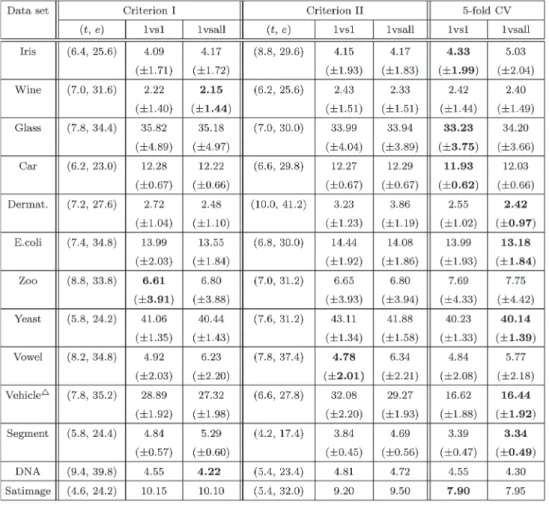
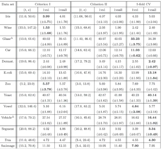
Table IV lists the results for the methods using the one-versus-one and one-versus-all strategies. The spherical GRBF kernel is employed. The columns are separated into three groups, showing the results from the two criteria and the five-fold cross validation, respectively. In the first two groups,tand
edenote the number of iterations and the number of function
evaluations, respectively. The “1vs1” and “1vsall” stand for the average test error rates from the methods of one-versus-one and one-versus-all, respectively. The numbers in the brackets are the standard deviations, and the minimal test error rates are highlighted in bold.
By comparing the test error rates, it is seen that for both multiclass SVM methods, the proposed criteria give rise to the classification performance comparable to that obtained by using the five-fold cross validation. For Criterion I, it achieves the minimal test error rate on “Wine,” “Zoo,” and “DNA.” On “Iris,” “Car,” “Dermatology,” “E.coli,” and “Yeast,” the test error rates are similar to those from the cross validation. Criterion I produces slightly higher error rates on “Glass,” “Vowel,” “Segment,” and “Satimage.” As for Criterion II, it is comparable to the cross validation on “Iris,” “Wine,” “Glass,” “Car,” “Zoo,” and “DNA.” On “Dermatology,” “E.coli,” “Yeast,” “Segment,” and “Satimage,” the test error rates from Criterion II are a bit higher. Comparison between the two criteria shows that Criterion I leads to slightly better overall classification performance. This can be seen from the data sets of “Dermatology,” “E.coli,” “Yeast,” and “DNA.” For both criteria, the test errors of the methods of “1vs1” and “1vsall” are comparable on most data sets; however, on “Vowel” and
TABLE IV
TESTERRORS(SPHERICALGRBF KERNEL, ONE-VERSUS-ONE,ANDONE-VERSUS-ALL)
“Segment,” the test error rates for the “1vsall” method are a bit higher. On the other hand, a failure of the model selection is also observed on “Vehicle,” where the obtained test error rates are significantly higher than that from the five-fold cross validation. This result can be expected from the discussion given at the end of Section VI-A1.
From the values oftande, it is known that the minimization process is often accomplished in a few iterations with a small number of function evaluations. For example, on “Iris,” when Criterion I is used, the model selection on a training subset completes in about seven iterations, including 26 function eval-uations in total. Referring to Table I, this means that 156(26× 2×3) QP problems are solved. However, for the five-fold cross-validation method, it has to solve 2700 (30×30×3)
QP problems when the one-versus-one strategy is used. Even if the grid number reduces to, for example, 10×10, by taking larger steps or by using a “coarse-to-fine” search, this number is still as high as 300.
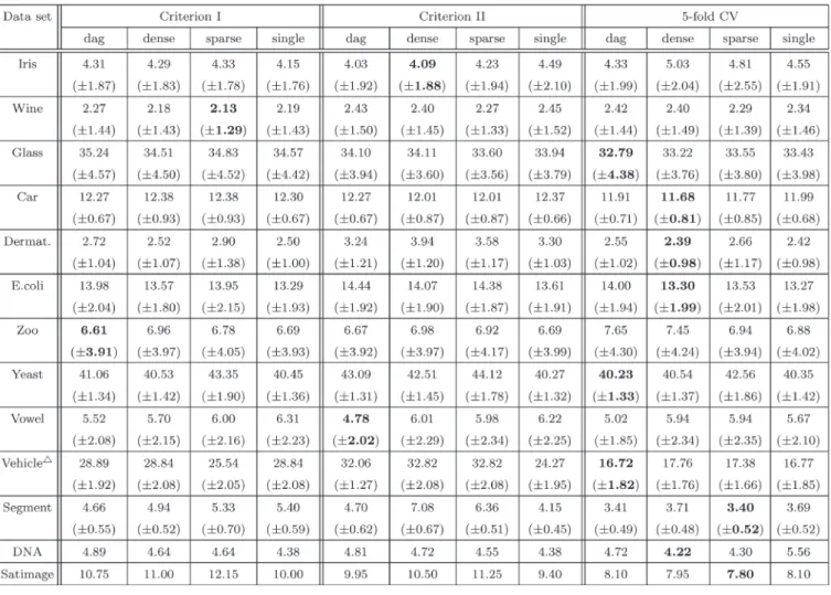
The results for the classification methods of “dag,” “dense,” “sparse,” and “single” are presented in Table V. The proposed criteria still provide good classification performance on most data sets except for “Vehicle.” In detail, Criterion I obtains min-imal test error rates on “Wine” and “Zoo,” whereas the test error rates on “Glass,” “Segment,” and “Satimage” are a little higher. For Criterion II, the test error rates are generally comparable to
those of the five-fold cross validation except that some increases are seen on “Dermatology,” “E.coli,” “Yeast,” “Segment,” and “Satimage.” With respect to the test error rate obtained by the five-fold cross validation, the maximum increase caused by using Criterion I is 4.35% on “Satimage” and that caused by using Criterion II is 3.89% on “Yeast.” Criterion I still shows marginally better classification performance than Criterion II. In addition, the test error rates listed in Tables IV and V are compared across the six classification methods. No strong evidence shows that Criteria I and II consistently perform better or worse on a particular method.
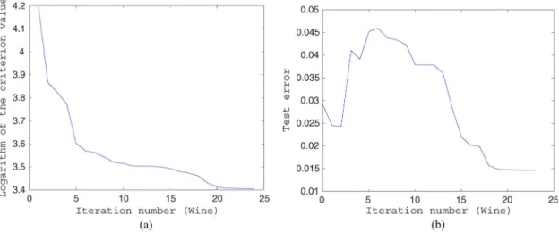
In short, it is observed from Tables IV and V that both criteria work well for the six classification methods. Although differences are observed between the test error rates obtained by the proposed criteria and those of the five-fold cross validation, they are not significant, particularly when the standard devi-ations are taken into account. Finally, to illustrate the details in a practical optimization process, the evolution of the values of Criterion I and the corresponding test error rate are shown in Fig. 5. As shown, the test error rate quickly drops with the decreasing criterion value.
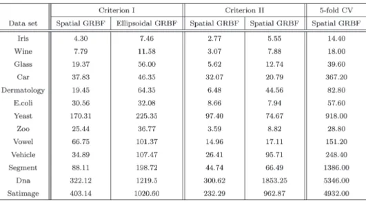
The following part presents the experimental results when the ellipsoidal GRBF kernel is employed. Considering that differentσvalues are assigned to each dimension, the number of model parameters increases to the feature dimensionality
TABLE V
TESTERRORS(SPHERICALGRBF KERNEL, DAG, DENSE, SPARSE,ANDSINGLE)
Fig. 5. Evolution of Criterion I and test error rate (Wine, spherical GRBF kernel). (a) Criterion value. (b) Test error rate.
plus one. In this case, even for the data represented by low-dimensional feature vectors, model selection with the exhaus-tive grid-based search methods becomes intractable.5 Both
5Considering that the five-fold cross-validation method is intractable for the case of multiple model parameters, the test errors obtained by using the spherical kernel have to be used in Table VI.
proposed criteria can still work well. As shown in Table VI, the minimization process still finishes in a number of itera-tions, although the number becomes larger due to more model parameters to be optimized. Compared with the case using a spherical kernel, lower test error rates are observed on “Iris,” “Wine,” “Car,” “Zoo,” and “Segment.” This may be the benefit of using an ellipsoidal kernel where feature components are
TABLE VI
TESTERRORS(ELLIPSOIDALGRBF KERNEL, ONE-VERSUS-ONE,ANDONE-VERSUS-ALL)
combined in a weighted fashion. Similar test error rates are obtained on “E.coli,” “Vowel,” and “DNA,” whereas higher error rates are seen on “Satimage.” The model selection per-formance of Criterion I is still better than that of Criterion II in general.
On the other hand, a degraded performance is seen on “Glass,” which is not as good as that obtained when a spherical kernel is used. Through analysis, we believe that this is because the number of training samples in some classes of “Glass” is so small (e.g., there are 2–6 training samples only) that the model selection process suffers from overfitting, i.e., when training samples are scarce, the minimization of the criteria may fit sample noise and fail to capture the real pattern there. In this case, although the minimum has been achieved, the selected model may not be good, and an SVM classifier using this model will not attain satisfactory classification performance on the test data. In addition, the model selection performance in this case often becomes sensitive to the optimization setting.6How to effectively avoid overfitting is also an active research area, and the regularization technique [31] seems to be a promising solution.
6With another optimization setting, we obtain a lower test error rate (33.96%±3.48%) on the “Glass” data set, which is comparable to that from the five-fold cross validation. However, the original result is reported for the sake of consistency of optimization settings for all the data sets.
Finally, Table VII presents the results from the “dag,” “dense,” “sparse,” and “single” methods. Similarly, on the data sets such as “Iris,” “Wine,” “Car,” and “Segment,” some decreases on test error rates are observed, whereas on the other data sets such as “Dermatology,” “Vowel,” and “Satimage,” the test error rates increase a bit. Generally speaking, for the case of using the ellipsoidal GRBF kernel, the proposed two criteria still demonstrate good performance for model selection in multiclass SVMs. There is no considerable scale performance degradation when the number of model parameters significantly increases, for example, to as high as 180 on “DNA.”
Before the end of this part, the model selection time taken by the proposed criteria is compared with that taken by the five-fold cross-validation approach. The comparison is carried out on a Linux server with 3.0-GHz CPU and 1.0-GB memory. In this experiment, the proposed criteria are computed and optimized by using the code written in Matlab. It calls the Linux binaries in LIBSVM to calculateR2andw2, and then loads the results from the output files. This is not the most efficient implementation in terms of computational time (for example, less efficient than realizing all the steps with a single
Cprogram). However, as shown in Table VIII, the two criteria have been able to achieve faster model selection than the five-fold cross-validation approach realized by using LIBSVM in
C. The model selection time for the ellipsoidal GRBF kernel is longer because more kernel parameters have to be optimized.
TABLE VII
TESTERRORS(ELLIPSOIDALGRBF KERNEL, DAG, DENSE, SPARSE,ANDSINGLE)
TABLE VIII
COMPARISON OF THEMODELSELECTIONTIME(UNIT: SECONDS)
This is particularly true for the data sets with high-dimensional input spaces. In addition, Criterion II generally costs less model selection time than Criterion I. They use different ways to evaluate the radiusR(solving a single larger quadratic problem
versus solving multiple smaller ones). However, it is believed that in practical applications, determining which criterion is faster will depend on the code design. The evolution of Cri-terion I and the corresponding test error rate is also shown in
Fig. 6. Evolution of Criterion I and test error rate (Wine, ellipsoidal GRBF kernel). (a) Criterion value. (b) Test error rate.
Fig. 6. At the initial stage, the criterion value decreases, but the test error rate increases. We believe that this is because the criterion is not a tight estimation of the test error rate. When the criterion value is relatively large, its decrease may not lead to an immediate reduction on the test error rate. However, as shown in Fig. 6, when the criterion value converges to its minimum, a lower enough test error rate will be achieved.
C. Application to Feature Selection
The optimized model parameters can be used to identify fea-tures important for classification.7For example, when the ellip-soidal GRBF kernel is used, the value ofgi(gi= 1/(2σ2i), i=
1,2, . . . , d) can reflect the importance of the ith feature, and the larger the gi value, the more important this feature is. This has been observed from the binary classification where the radius–margin bound is applicable [16]. This experiment will demonstrate that the proposed criteria well preserve this property in multiclass classification. Two data sets are used. One is a toy problem, and the other is the U.S. Postal Service (USPS) data set on optical digit recognition.
1) Toy Data Set: This data set is created by following [16]. However, in this experiment it consists of multiple classes. There are 52 features in total, and only the first two of them are useful. The two features are shown in Fig. 7(a). There are three concentric circles, forming a three-class classification prob-lem. The remaining 50 features are randomly sampled from a Gaussian distribution ofN(0,20). Three hundred samples are generated in total. This experiment is to check whether the first two features can be identified by using the proposed criteria, i.e., being assigned largergvalues. The toy data set is randomly split into 100 pairs of training/test subsets, and Criterion II is applied to each of the training subsets. Considering that the three classes are completely nonlinearly separable, the initial
7Please note that the feature selection here is different from feature extraction that considers the feature dependence and seeks the optimal combination of features, for example, in the way of principal component analysis or linear dis-criminant analysis. Here, features are treated individually, and those important for classification are identified. As for the feature dependence, it is left to the SVM classifier that can handle it automatically.
value of the regularization parameter C is set as a bit higher value, e.g., 10.0. A promising result is obtained. The first two features are correctly assigned higher g values on all the 100 trials. The g values averaged over the 100 trials are shown in Fig. 7(b). As shown, the first two features can be easily identified by sorting the g values. Once they are correctly selected, the three circles can be classified without error. It is assumed here that “only two features are really useful” is known beforehand. In a general case, the top k features will be selected, and some noisy features will be brought in ifkis larger than the number of useful features, for example, two for this data set.
2) Optical Digit Recognition: The USPS data set contains 7291 training samples and 2007 test samples. They form ten classes corresponding to digits from “0” to “9.” Each sample is characterized by a 256-D feature vector. It is obtained by re-shaping a 16×16 gray-level thumbnail image. Some examples are shown in Fig. 8.
With the training data, the proposed criteria are minimized to find the optimal model parameters. Afterward, the multiclass SVMs with the optimized model parameters are created and evaluated. The test error rates are listed in Table IX. The value in the column of “Reported best” is the lowest test error rate given in [32] when a spherical GRBF kernel is used (that for an ellipsoidal GRBF kernel is left blank because the five-fold cross-validation approach is intractable in this case). As seen from this table, the multiclass SVMs with the optimized model parameters give rise to the classification performance comparable to the reported best. When the ellipsoidal kernel is used, slightly increased test error rates are observed, but the difference between our results and the reported best is still less than 1%.
By reshaping the optimal value ofg1, g2, . . . , g256back into a 16×16 matrix, the map ofgvalues is shown in Fig. 9, where each block corresponds to one of the 256g’s and its magnitude is reflected by the gray value. The blocks having largergvalues distribute at the central part of this map, whereas those having lower values are mostly at the borders and corners. This result implies that the pixels at the central part are more important for classification. This result well matches the case of the
Fig. 7. Results for the toy data set. (a) Distribution of the first two features. (b) Optimized value ofg= 1/(2σ2)averaged on 100 trails.
Fig. 8. Thumbnail images of digits (USPS data set).
TABLE IX
TESTERRORSOBTAINEDWITH THESELECTEDMODELPARAMETERS(THEUSPS DATASET)
Fig. 9. Map of optimized values ofg(USPS data set). (a) Criterion I. (b) Criterion II.
thumbnail images in Fig. 8 that a digit is commonly displayed at the central part of an image.8To investigate the performance of feature selection using thesegvalues, the following experi-ments are conducted. The 256 features are sorted according to a descending order of the correspondinggvalues, and only the topk features are used to train a multiclass SVM to perform
8This experiment was first presented in [16], where a binary classification problem of discriminating two groups of digits (group I, “0”–“4”; group II: “5”–“9”) is considered and the radius–margin bound is used. This paper develops two model selection criteria and makes such a feature selection applicable to the multiclass classification that discriminates each digit from each other.
classification. For comparison, another three feature selection methods named “Fisher criterion score,” “Pearson correlation coefficient,” and “Kolmogorov–Smirnov test” in [16] are also used and adapted to the multiclass case. The following two points will be checked: 1) whether the test error rate rapidly decreases with the increasing value of k, and 2) whether the proposed criteria can produce feature selection performance comparable to the other three methods. The result is shown in Fig. 10, where the horizontal axis is the number of selected features and the vertical one is the test error rate. It is seen that the test error rate drops quickly with the increasing number of selected features. Compared with the other three methods,
Fig. 10. Feature selection result. Test error rate versus number of selected features (USPS data set).
both criteria give better feature selection performance. By using only the top 50 selected features, the test error rate of 0.07 has been achieved (the lowest error rate is about 0.05 when all the 256 features are used). Many redundant features are recognized by using the proposed criteria. The curves in Fig. 10 show the change of test error rate with respect to the number of selected features. In practical applications, a point on the curve can be selected to balance between classification accuracy and the number of features used in an SVM classifier.
D. Summary
Based on the aforementioned experimental results, the fol-lowing summary can be made.
1) Both criteria demonstrate good model selection perfor-mance on most of the data sets, giving rise to classifica-tion accuracy comparable to that obtained by using the five-fold cross-validation approach.
2) The two criteria work well with both spherical and ellip-soidal GRBF kernels, and the latter verifies their ability in handling a large number of model parameters. At the same time, it is also observed that satisfactory model selection may not be attained if training samples are scarce. How to solve this problem is still an ongoing research, and it is worth exploring in future work. 3) Six different kinds of multiclass SVM methods are
in-vestigated. Although the proposed criteria are developed on the multiclass SVM using the one-versus-one strategy, they help all the six multiclass SVM classifiers achieve good enough classification performance. It seems that the two criteria are promising to be generally used for model selection of multiclass SVM methods.
4) Model parameters optimized by the two criteria are used to do feature selection. Compared with the existing se-lection criteria, they achieve comparable or even better selection results. We believe that this property has wide applications in real-world problems and that it is worth further investigation.
5) The comparison of the two criteria finds that Criterion I shows marginally better performance. Meanwhile, there
is a difference between their computational loads. To compute the radiusR2, Criterion I solves multiple smaller scale QP problems, whereas Criterion II solves one larger scale QP problem. When the number of classes is large, model selection with the second criterion might be faster.
VII. CONCLUSION
This paper has proposed two criteria to perform model selection in multiclass SVMs. They are realized by combining or redefining the radius–margin bound of binary classification to accommodate multiple classes. Both criteria are not the radius–margin bound generalized for multiclass SVMs. Nev-ertheless, they are simple and practical, and most importantly, they demonstrate satisfactory performance in the task of model selection for which they are proposed. These two criteria well preserve the elegant properties of the radius–margin bound in the model selection of binary SVMs. Their derivatives with respect to model parameters are analytically calculated, and thus, the gradient-based optimization technique is used to find the best model efficiently. The two criteria handle hundreds of model parameters well and save much computational cost than the grid-based search methods. In addition, they do not need to put a part of training samples aside for validation and make full use of all the training samples available. In the application to feature selection, the optimized model parameters success-fully identify features important for classification. This is very helpful for the reduction of system complexity and feature dis-covery. Extensive experimental study on multiple benchmark data sets and different multiclass SVM methods verify the effectiveness of the proposed criteria and their applicability for multiclass SVM model selection.
REFERENCES
[1] R. Rifkin and A. Klautau, “In defense of one-vs-all classification,”
J. Mach. Learn. Res., vol. 5, pp. 101–141, Dec. 2004.
[2] J. H. Friedman, “Another approach to polychotomous classification,” Dept. Stat. Stanford Linear Accelerator Center, Stanford Univ., Stanford, CA, 1996. Tech. Rep.
[3] U. Kressel, “Pairwise classification and support vector machines,” in
Advances in Kernel Methods—Support Vector Learning, B. Schölkopf, C. Burges, and A. J. Smola, Eds. Cambridge, MA: MIT Press, 1999. [4] T. Dietterich and G. Bakiri, “Solving multiclass learning problems via
error-correcting output codes,”J. Artif. Intell. Res., vol. 2, pp. 263–286, 1995.
[5] E. L. Allwein, R. E. Schapire, and Y. Singer, “Reducing multiclass to binary: A unifying approach for margin classifiers,”J. Mach. Learn. Res., vol. 1, pp. 113–141, 2000.
[6] J. Weston and C. Watkins, “Support vector machines for multi-class pattern recognition,” inProc. 7th Eur. Symp. Artif. Neural Netw., 1999, pp. 219–224.
[7] K. Crammer and Y. Singer, “On the learnability and design of output codes for multiclass problems,” inProc. 13th Annu. Conf. Comput. Learn. Theory, 2000, pp. 35–46.
[8] Y. Lee, Y. Lin, and G. Wahba, “Multicategory support vector machines,” inProc. 33rd Symp. Interface Comput. Sci. Statist., 2001, pp. 498–512. [9] C.-W. Hsu and C.-J. Lin, “A comparison of methods for multiclass support
vector machines,”IEEE Trans. Neural Netw., vol. 13, no. 2, pp. 415–425, Mar. 2002.
[10] W.-C. Kao, K.-M. Chung, C.-L. Sun, and C.-J. Lin, “Decomposition methods for linear support vector machines,”Neural Comput., vol. 16, no. 8, pp. 1689–1704, Aug. 2004.
[11] P.-H. Chen, C.-J. Lin, and B. Schölkopf, “A tutorial onν-support vector machines,”Appl. Stoch. Models Bus. Ind., vol. 21, no. 2, pp. 111–136, 2005.