Deutsches Institut für Wirtschaftsforschung
www.diw.de
Michal Myck
•Richard Ochmann
•Salmai Qari
S
R
Dynamics of Earnings and Hourly
Wages in Germany
1
3
9
SOEPpapers
on Multidisciplinary Panel Data Research
SOEPpapers on Multidisciplinary Panel Data Research
at DIW Berlin
This series presents research findings based either directly on data from the German Socio-Economic Panel Study (SOEP) or using SOEP data as part of an internationally comparable data set (e.g. CNEF, ECHP, LIS, LWS, CHER/PACO). SOEP is a truly multidisciplinary household panel study covering a wide range of social and behavioral sciences: economics, sociology, psychology, survey methodology, econometrics and applied statistics, educational science, political science, public health, behavioral genetics, demography, geography, and sport science.
The decision to publish a submission in SOEPpapers is made by a board of editors chosen by the DIW Berlin to represent the wide range of disciplines covered by SOEP. There is no external referee process and papers are either accepted or rejected without revision. Papers appear in this series as works in progress and may also appear elsewhere. They often represent preliminary studies and are circulated to encourage discussion. Citation of such a paper should account for its provisional character. A revised version may be requested from the author directly.
Any opinions expressed in this series are those of the author(s) and not those of DIW Berlin. Research disseminated by DIW Berlin may include views on public policy issues, but the institute itself takes no institutional policy positions.
The SOEPpapers are available at
http://www.diw.de/soeppapers
Editors:
Georg Meran (Vice President DIW Berlin) Gert G. Wagner (Social Sciences)
Joachim R. Frick (Empirical Economics) Jürgen Schupp (Sociology)
Conchita D’Ambrosio (Public Economics)
Christoph Breuer (Sport Science, DIW Research Professor) Anita I. Drever (Geography)
Elke Holst (Gender Studies)
Frieder R. Lang (Psychology, DIW Research Professor) Jörg-Peter Schräpler (Survey Methodology)
C. Katharina Spieß (Educational Science) Martin Spieß (Survey Methodology)
Alan S. Zuckerman (Political Science, DIW Research Professor)
ISSN: 1864-6689 (online)
German Socio-Economic Panel Study (SOEP) DIW Berlin
Mohrenstrasse 58 10117 Berlin, Germany
Dynamics of Earnings and Hourly
Wages in Germany
∗
Michał Myck
†Richard Ochmann
‡Salmai Qari
§October 27, 2008
Abstract
There is by now a vast number of studies which document a sharp increase in cross-sectional wage inequality during the 2000s. It is often assumed that this inequality is of a “permanent nature” which in turn is used as an argument calling for government interven-tion. We examine these claims using a fully balanced panel of full-time employed individ-uals in Germany from the German Socio-Economic Panel for the years 1994-2006. In line with previous studies, our sample shows sharply rising inequality during the 2000s. Ap-plying covariance structure models, we calculate the fraction of permanent and transitory wage and earnings inequality. From 1994 on, permanent inequality increases continuously, peaks in 2001 and then declines in subsequent years. Interestingly the decline in the per-manent fraction of inequality occurs at the time of most rapid increases in cross-sectional inequality. It seems therefore that it is primarily the temporary and not the permanent component which has driven the strong expansion of cross-sectional inequality during the 2000s in Germany.
Keywords: Variance Decomposition, Covariance Structure Models, Earnings Inequality, Wage Dynamics.
JEL Classification: C23, D31, J31
∗We thank Benny Geys and Viktor Steiner for helpful comments. The usual disclaimer applies. Qari gratefully acknowledges financial support from the Anglo-German Foundation through the CSGE research initiative. †German Institute for Economic Research (DIW Berlin), Institute for Fiscal Studies, and IZA-Bonn, e-mail:
‡German Institute for Economic Research (DIW Berlin), e-mail: [email protected] §Social Science Research Center Berlin (WZB), e-mail: [email protected]
1 Introduction
The evolution of wage inequality in Germany is commonly perceived to approach the dynamics of the U.S. labour market in recent years. The literature on cross-sectional wage and earnings inequality in Germany typically finds that the wage distribution was stable during the 1980s and inequality started to increase in the middle of the 1990s.1 Moreover, this increase steepens in the 2000s (Gernandt and Pfeiffer, 2007; Müller and Steiner, 2008). However, a pure cross-sectional approach is unable to identify the dynamics of the respective distributions and as such is not very informative about the mechanism determining the changes. A rise in cross-sectional inequality over time might result from an increasing role of temporary shocks or from growing permanent differences in wages and earnings between individuals. Thus, cross-sectional studies are unable to distinguish between “transitory” and “permanent” inequality. From a policy perspective it is however clearly important to disentangle the two sources of inequality, as it greatly affects the role of government interventions applied to mitigate inequality.
We apply covariance structure models to longitudinal data from the German Socio-Economic Panel (GSOEP) for the years 1994-2006. This allows us to decompose the cross-sectional dispersion into its permanent and transitory elements. Models of this type were used to analyse the wage and earnings structure of the United States (Moffitt and Gottschalk, 2002), Canada (Baker and Solon, 2003) and the UK (Dickens, 2000).2 Using a similar approach, Biewen (2005)
analyses the evolution of disposable household income inequality in East- and West-Germany for the years 1990-1998. He finds a slightly decreasing part of permanent variance for West-Germany compared to a strongly increasing part of permanent variance for East-West-Germany in these years. Daly and Valletta (2008) use a heterogeneous growth model to compare Germany, UK and the USA during the 1990s. For these three countries they find substantial convergence in the permanent and transitory parts of inequality, mainly caused by an increase in permanent inequality in Germany and a decline of permanent inequality in the United States. Burkhauser and Poupore (1997) and Maasoumi and Trede (2001) compare the United States and Germany during the 1980s in terms of permanent and transitory inequality with different approaches.
We are however not aware of any study covering the longitudinal dimension of earnings and wage inequality in Germany beyond the year 2000. As the increase in cross-sectional inequality steepens in the 2000s (see, for example, Gernandt and Pfeiffer, 2007) it is important to identify 1While there is agreement on the expansion of inequality during the 1990s, there is some disagreement about the 1980s. In a recent paper Dustmann et al. (2007) challenge “the view that the wage structure in West-Germany has remained stable throughout the 80s and 90s. Based on a 2 % sample of social security records, [they] show that wage inequality has increased in the 1980s, but only at the top of the distribution.” 2For earlier examples, see Lillard and Willis (1978), Lillard and Weiss (1979), as well as Abowd and Card
(1989). For a study covering Italy, see Cappellari (2000). Gustavsson (2007) provides a recent study applying Swedish data.
how much of this increase can be attributed to changes in the permanent component.
Our main results are threefold. Firstly, the cross-sectional variance in our sample increases – depending on the specification– by 20 to 50 percent from 1994 to 2006. Consistent with previous research, our sample shows that the increase is much steeper in the 2000s. In fact, most of the increase occurs between 1999 and 2006, while from 1994 to 1999 the cross-sectional variance remains relatively stable. Secondly, the rise in the cross-sectional variance is accompanied by an increase in the fraction of its permanent part. Interestingly, this increase also shows a break around the years 2000/2001. While the fraction of the permanent inequality increases from 1994 to 2000 and peaks in 2001, it then declines from there on by approximately 20 percentage points. This implies that the strong expansion of cross-sectional inequality during the 2000s can be increasingly attributed to transitory inequality. Finally, we find virtually no difference between the evolution of earnings and wage inequality in the period from 1994 to 2006. This is to a large extent a consequence of our focus on full-time employees, but reflects also a relatively compressed distribution of working hours in Germany compared the United States and the UK (Burton and Phipps, 2007).
In the following section we describe the dataset we use for our analysis. Section 3 presents the method for separating the permanent and temporary components of the variance. Section 4 provides details on the estimation procedure. We then present and discuss our main results in Section 5 and conclude in Section 6.
2 Data
The analysis uses data from the German Socio-Economic Panel (GSOEP). The GSOEP is a panel study for Germany, which was started in 1984 as a longitudinal survey of households and individuals in West-Germany and was expanded in 1990 to cover the population of the former East Germany. We use a fully balanced subsample of the GSOEP for the years 1994-2006. Thus, we focus on individuals from the first four samples (A, B, C, and D) of the GSOEP in order to make analyses between any two periods of the time frame comparable.3
We apply the usual age restrictions and include individuals aged 20-60 who report to be “employed” in all 13 years covered by the analysis and who are full-time employees during the entire period.4 For these individuals, we analyse monthly gross individual labour income as 3Sample A and B are the initial samples with residents in the former Federal Republic of Germany from households with a German household head as well as households with heads from Turkey, Greece, Yugoslavia, Spain, or Italy. Sample C was started in 1990 with German residents from private households in the former German Democratic Republic. Sample D was started in 1994 with immigrants. These samples of the GSOEP are multi-stage random samples, which are regionally clustered. C.f. Haisken-DeNew and Frick (2005) and Wagner et al. (2007) for further details.
reported for the month prior to the interview. Earnings are deflated by Consumer Price Index to the base of year 2000.5 To exclude outliers, the distribution of monthly earnings is truncated
at 100 Euros at the low end and 20,000 Euros at the high end.6
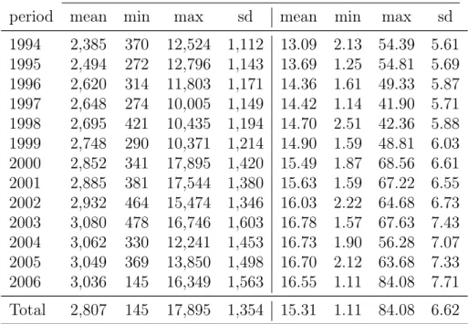
Table 1: Summary Statistics for Earnings and Wages Monthly Earnings Hourly Wages
period mean min max sd mean min max sd
1994 2,385 370 12,524 1,112 13.09 2.13 54.39 5.61 1995 2,494 272 12,796 1,143 13.69 1.25 54.81 5.69 1996 2,620 314 11,803 1,171 14.36 1.61 49.33 5.87 1997 2,648 274 10,005 1,149 14.42 1.14 41.90 5.71 1998 2,695 421 10,435 1,194 14.70 2.51 42.36 5.88 1999 2,748 290 10,371 1,214 14.90 1.59 48.81 6.03 2000 2,852 341 17,895 1,420 15.49 1.87 68.56 6.61 2001 2,885 381 17,544 1,380 15.63 1.59 67.22 6.55 2002 2,932 464 15,474 1,346 16.03 2.22 64.68 6.73 2003 3,080 478 16,746 1,603 16.78 1.57 67.63 7.43 2004 3,062 330 12,241 1,453 16.73 1.90 56.28 7.07 2005 3,049 369 13,850 1,498 16.70 2.12 63.68 7.33 2006 3,036 145 16,349 1,563 16.55 1.11 84.08 7.71 Total 2,807 145 17,895 1,354 15.31 1.11 84.08 6.62
Source: Own calculations using the GSOEP data (1994-2006).
To compute hourly wages, we use reported weekly hours actually worked (including hours of paid overtime) and monthly earnings (including overtime pay).7 The distribution of the
resulting hours worked is censored at 84 hours per week. The resulting hourly wage is then
employees.
5Note, however, that a deflation of this variable does not affect the analysis of variances later on, since a common factor just alters the level, which in turn does not alter our measure of dispersion.
6Although the GSOEP is not generally top-coded with respect to the income distribution, it nevertheless in-cludes only a small number of individuals with high incomes in the samples A-D applied here, c.f. Dustmann et al. (2007), Bach et al. (2007) as well as Bach et al. (2008). These authors moreover conclude that the GSOEP covers the distribution of market income quite well up to the 99th percentile. Bach et al. (2007) also find that a large share of the total market income is actually labour income, in 2001 a share of 83.1 percent on average was wage income and an additional 11.4 percent was income from business activity. We conclude that by analysing labour earnings we capture the main part of market income which is representative for the income distribution in Germany, except for the very rich.
7In several cases of missings at the hours, namely 191 individual-year observations, generally mean hours by employment status and year are imputed.
calculated as wage = monthly earnings / (4.35 * weekly hours worked). Table 1 displays some descriptive statistics on monthly earnings and hourly wages in our sample of analysis.
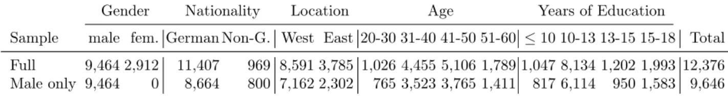
Table 2: Number of Individual-Year Observations in the Samples
Gender Nationality Location Age Years of Education
Sample male fem. German Non-G. West East 20-30 31-40 41-50 51-60 ≤1010-13 13-15 15-18 Total Full 9,464 2,912 11,407 969 8,591 3,785 1,026 4,455 5,106 1,789 1,047 8,134 1,202 1,993 12,376 Male only 9,464 0 8,664 800 7,162 2,302 765 3,523 3,765 1,411 817 6,114 950 1,583 9,646
Source: Own calculations using the GSOEP data (1994-2006).
Although we use different sets of control variables we keep only those observations which do not have any missing information for the full set of covariates. The restrictions lead to an overall sample of 952 individuals (12,376 individual-year observations). When we restrict the sample only to men we end up with 728 individuals (9,464 individual-year observations). Table 2 displays the number of individual-year observations by gender, nationality, location as well as by age and education groups for our balanced panel on the full sample and for the one restricted to men only.
3 Modelling the Dynamics of Earnings and Wages
We assume that real log-earnings (log-wages, respectively) can be modelled by
Yit =x0itβt+uit (1)
for individualsi= 1, ...N and periodst = 1, ...T, withxitdenoting aK×1-vector of individual-specific characteristics including a time-varying constant, βt denoting a K ×1 time-varying parameter vector, and uit the error term. This model is computed for every t = 1, ...T in two variants. In the first variant, xit ≡1, so that log earnings are only regressed on a time-varying constant. In the second variant, xit contains several individual-specific covariates, i.e. log-age, log-age-squared, region of residence (East- or West-Germany), years of education in four groups, and gender for the full sample of males and females.
For each variant, we decompose the residuals uit into a permanent and a transitory part. Throughout the entire paper we assume that these two parts are uncorrelated, i.e. Cov(µi, vit) =
0.
Our simplest model is the “enhanced canonical” permanent-transitory model with year-specific factor loadings pt and λt on the two components. It assumes that there is no serial
correlation among transitory shocks, i.e Cov(vit, vit−s) = 0 for s6= 0:8
uit=ptµi+λtvit (2)
Intuitively,x0itβt defines the population’s mean profile and the termµi introduces individual heterogeneity, which allows the individuals to deviate from the mean profile. The variance of this individual heterogeneity constitutes the source for permanent inequality and the respective factor loadings allow changes of the permanent component over time.
The variance of the residual of log-earnings (log-wages, respectively) in this model, given independence of the permanent and the transitory component, is:
V ar(uit) = p2tσ 2 µ+λ 2 tσ 2 v (3)
An increase in either factor loading in period t leads to an increase in the cross-sectional variance of periodt. The interpretation of such an increase, however depends crucially on which factor changes. An increase inptcan be interpreted as an increase in the returns to unobserved individual-specific permanent components, e.g. ability. On the contrary, an increase in λt without an increase in pt can be interpreted as an increase in year-to-year volatility due to short-term factors, such as e.g. temporarily powerful labour unions or demand shocks affecting specific sectors of the economy, without any shifts in the permanent component of earnings.
To remove the implausible assumption that temporary shocks do not have any effect on the following periods, we consider two models for the transitory component. The first model is an AR(1) process. In this case, the transitory part of the residuals is equal to:
vit =ρvit−1+εit (4)
In the second model, the transitory component is assumed to follow an ARMA(1,1) process: vit =ρvit−1+γεit−1+εit (5)
Under the assumption that E[µi] =E[vit] =E[εit] = 0 and E[µiεit] = E[εitεjs] = 0 for all i and j and for all t6=s, the covariance matrix of residuals is given by:
cov(uit, uit−s) = ptpt−sσµ2 +λtλt−sE[vitvit−s] (6)
8C.f. Moffitt and Gottschalk (2002), Baker and Solon (2003), and Haider (2001) for other applications of such a model.
where pt, pt−s, λt, and λt−s are time specific factor loadings and E[vitvit−s] is equal to: E[vitvit−s] = σ2 v0 , t= 0, s= 0 ρ2σ2 v0+σ2 , t= 1, s= 0 ρ2E[v it−1vit−1] + (1 +γ2+ 2ργ)σ2 ,2≤t, s = 0 ρs−1(ρE[v it−svit−s] +γσ2) , s+ 1≤t,1≤s≤T −1 (7) In Equation (7), σ2
µ = var(µi) and σε2 = var(εit).9 σv20 = var(vi0) is the initial condition for the ARMA-process.10 In Equation (7), the AR(1) specification is nested with γ = 0.
Summarising, we consider three different specifications:
(S-CAN) uit =ptµi+λtvit (8)
(S-AR) uit =ptµi+λt(ρvit−1+εit) (9) (S-ARMA) uit =ptµi+λt(ρvit−1+γεit−1+εit) (10)
Specification (S-CAN) is the “enhanced canonical” model with factor loadings. Specification (S-AR) models the transitory component as an AR(1) process, while specification (S-ARMA) models the transitory component as an ARMA(1,1) process. (S-CAN) is nested in (S-AR) which in turn is nested in (S-ARMA).
4 Estimation
The estimation is conducted in two steps.11 In the first step, we obtain an estimate of uit, which is just the vector of residuals from the regression model Yit = x0itβt +uit. From these residuals, we construct an empirical covariance matrix.12 In the second step, we estimate the parameters of our theoretical covariance matrix by fitting the implications of specifications (S-CAN), (S-AR), and (S-ARMA) to the empirical covariance matrix.
Formally, let the vectorC collect all distinct elements of the empirical covariance matrix ob-tained from the first stage. For each specification, we can express the corresponding theoretical moments in Equations (6)-(7) as a function f(θ), where the vector θ collects all parameters which are needed to construct these moments. For example, in specification (S-AR), θ col-lects the initial variance, as well as the permanent variance, the year-to-year variance, the
9See Biewen (2005) for similar specifications in the context of household income.
10The initial condition is needed for an unbiased estimation of the parameters of the ARMA-process, c.f. MaCurdy (1982).
11C.f. MaCurdy (1982); Haider (2001); Biewen (2005).
persistence parameter of the AR(1) process, and the factor loadings for the permanent and transitory components. This results in 27 parameters for specification (S-AR) and 28 for spec-ification (S-ARMA), respectively.13 The model’s parameters are estimated by the generalised
method of moments (Chamberlain, 1984); that is the estimateθˆminimises the distance between the empirical and the theoretical moments:
ˆ
θ = arg min
θ [C−f(θ)]
0
W[C−f(θ)] (11)
We follow the recent literature and use the identity matrix as the weighting matrixW.14 This approach, called “equally weighted minimum distance estimation” (Baker and Solon, 2003), boils down to using nonlinear least squares to fit f(ˆθ)to C.
5 Results
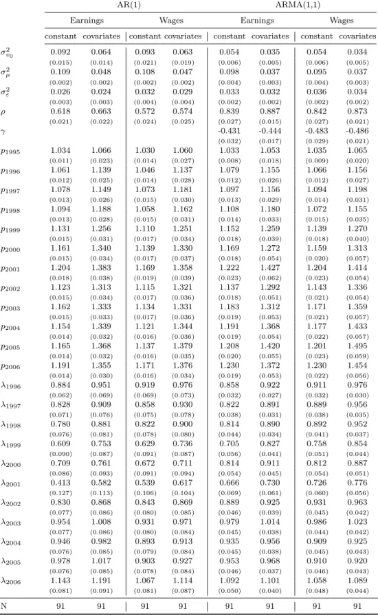
The estimation results are compiled in Table 3. It shows the 27 (28, respectively) parameter estimates for the specifications (S-AR) and (S-ARMA). These results are obtained from the full sample.15 The distribution of working hours for full-time employees is fairly constant over
time. As a consequence, the evolution of earnings dynamics in our sample closely resembles the one for wage dynamics. We therefore focus on the results for wages here.
In specification (S-AR), the variance of the transitory part (σε2) for wages is estimated to between one third and two thirds of the permanent variance (σµ2). Meanwhile, transitory shocks die out rather quickly. An estimate for ρ of 0.57 implies that already after two periods almost 70% of a shock are vanished. Also in specification (S-ARMA), the persistence of transitory shocks is relatively modest with an estimatedρof about0.85and aγof about−0.48. Similarly, this implies that a shock is reduced to about 31% after two periods. The evolution of the factor loadings (pt) suggests that the permanent component becomes increasingly important during the years 1994 to 2001. In line with that, the factor loadings of the transitory part (λt) are initially only slightly below unity, then decline continuously until the year 2001, whereupon until 2006, they grow sharply up to slightly above unity.
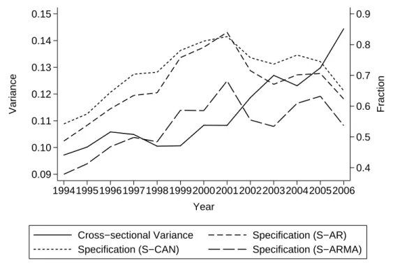
We can now use Equation (6) and calculate the fraction of the permanent part of the variance from our parameter estimates as (ˆp2
t·σˆ2µ)/ var(ˆuit), where var(ˆuit)denotes the variance of the predicted residuals in periodt. Figure 1 shows the evolution of this fraction for wages regressed
13Note thatp
1994,λ1994andλ1995 are normalised to unity in order to identify the parameters of the stochastic
process.
14While an asymptotically optimal choice of W is the inverse of a matrix that consistently estimates the covariance matrix of C (Chamberlain, 1984), Altonji and Segal (1996) as well as Clark (1996) provide Monte Carlo evidence of potentially serious finite sample bias inθˆusing this approach.
Table 3: Parameter Estimates - Full Sample
AR(1) ARMA(1,1)
Earnings Wages Earnings Wages constant covariates constant covariates constant covariates constant covariates
σ2 v0 0.092 0.064 0.093 0.063 0.054 0.035 0.054 0.034 (0.015) (0.014) (0.021) (0.019) (0.006) (0.005) (0.006) (0.005) σ2 µ 0.109 0.048 0.108 0.047 0.098 0.037 0.095 0.037 (0.002) (0.002) (0.002) (0.002) (0.004) (0.003) (0.004) (0.003) σ2 ε 0.026 0.024 0.032 0.029 0.033 0.032 0.036 0.034 (0.003) (0.003) (0.004) (0.004) (0.002) (0.002) (0.002) (0.002) ρ 0.618 0.663 0.572 0.574 0.839 0.887 0.842 0.873 (0.021) (0.022) (0.024) (0.025) (0.027) (0.015) (0.027) (0.021) γ -0.431 -0.444 -0.483 -0.486 (0.032) (0.017) (0.029) (0.021) p1995 1.034 1.066 1.030 1.060 1.033 1.053 1.035 1.065 (0.011) (0.023) (0.014) (0.027) (0.008) (0.018) (0.009) (0.020) p1996 1.061 1.139 1.046 1.137 1.079 1.155 1.066 1.156 (0.012) (0.025) (0.014) (0.028) (0.012) (0.026) (0.012) (0.027) p1997 1.078 1.149 1.073 1.181 1.097 1.156 1.094 1.198 (0.013) (0.026) (0.015) (0.030) (0.013) (0.029) (0.014) (0.031) p1998 1.094 1.188 1.058 1.162 1.108 1.180 1.072 1.155 (0.013) (0.028) (0.015) (0.031) (0.014) (0.033) (0.015) (0.035) p1999 1.131 1.256 1.110 1.251 1.152 1.259 1.139 1.270 (0.015) (0.031) (0.017) (0.034) (0.018) (0.039) (0.018) (0.040) p2000 1.161 1.340 1.139 1.330 1.169 1.272 1.159 1.313 (0.015) (0.034) (0.017) (0.037) (0.018) (0.054) (0.020) (0.057) p2001 1.204 1.383 1.169 1.358 1.222 1.427 1.204 1.414 (0.018) (0.038) (0.019) (0.039) (0.023) (0.062) (0.023) (0.054) p2002 1.123 1.313 1.115 1.321 1.137 1.292 1.143 1.336 (0.015) (0.034) (0.017) (0.036) (0.018) (0.051) (0.021) (0.054) p2003 1.162 1.333 1.134 1.331 1.183 1.312 1.171 1.359 (0.015) (0.033) (0.017) (0.036) (0.019) (0.053) (0.021) (0.057) p2004 1.154 1.339 1.121 1.344 1.191 1.368 1.177 1.433 (0.014) (0.032) (0.016) (0.036) (0.019) (0.054) (0.022) (0.057) p2005 1.165 1.368 1.137 1.379 1.208 1.420 1.201 1.495 (0.014) (0.032) (0.016) (0.035) (0.020) (0.055) (0.023) (0.059) p2006 1.191 1.355 1.171 1.376 1.230 1.372 1.230 1.454 (0.014) (0.030) (0.016) (0.034) (0.019) (0.053) (0.022) (0.056) λ1996 0.884 0.951 0.919 0.976 0.858 0.922 0.911 0.976 (0.062) (0.069) (0.069) (0.073) (0.032) (0.027) (0.032) (0.030) λ1997 0.828 0.909 0.858 0.930 0.822 0.891 0.889 0.956 (0.071) (0.076) (0.075) (0.078) (0.038) (0.031) (0.038) (0.035) λ1998 0.780 0.881 0.822 0.900 0.814 0.890 0.892 0.952 (0.076) (0.081) (0.078) (0.080) (0.044) (0.034) (0.041) (0.037) λ1999 0.609 0.753 0.629 0.736 0.705 0.827 0.758 0.854 (0.090) (0.087) (0.091) (0.087) (0.056) (0.041) (0.051) (0.044) λ2000 0.709 0.761 0.672 0.711 0.814 0.911 0.812 0.887 (0.086) (0.093) (0.091) (0.094) (0.054) (0.045) (0.054) (0.051) λ2001 0.413 0.582 0.539 0.617 0.666 0.730 0.726 0.776 (0.127) (0.113) (0.106) (0.104) (0.069) (0.061) (0.060) (0.056) λ2002 0.830 0.868 0.843 0.869 0.889 0.925 0.931 0.963 (0.077) (0.086) (0.080) (0.085) (0.046) (0.039) (0.045) (0.042) λ2003 0.954 1.008 0.931 0.971 0.979 1.014 0.986 1.023 (0.077) (0.086) (0.080) (0.084) (0.045) (0.038) (0.044) (0.042) λ2004 0.946 0.982 0.893 0.913 0.935 0.956 0.909 0.925 (0.076) (0.085) (0.079) (0.084) (0.045) (0.038) (0.045) (0.043) λ2005 0.978 1.017 0.903 0.927 0.953 0.968 0.910 0.920 (0.076) (0.085) (0.078) (0.084) (0.046) (0.037) (0.046) (0.043) λ2006 1.143 1.191 1.067 1.114 1.092 1.101 1.058 1.089 (0.081) (0.091) (0.081) (0.087) (0.050) (0.040) (0.048) (0.044) N 91 91 91 91 91 91 91 91
Notes: See Section 3 for the full list of covariates.
on the full set of covariates for all three specifications.16 It also includes the cross-sectional
variance var(uit).
Figure 1: Cross-sectional Variance and its Permanent Component, for Wages in the specifica-tion with covariates on the full sample
0.4 0.5 0.6 0.7 0.8 0.9 Fraction 0.09 0.10 0.11 0.12 0.13 0.14 0.15 Variance 1994199519961997199819992000200120022003200420052006 Year
Cross−sectional Variance Specification (S−AR)
Specification (S−CAN) Specification (S−ARMA)
Notes: See Section 3 for the full list of covariates.
The plots show a clear break in the years 2000/2001. From 1994 to 1999, the cross-sectional variance is more or less constant, followed by a sharp increase starting in 2000. This sharp increase in cross-sectional inequality is in line with previous research as mentioned earlier. However, the permanent part of the variance increases sharply only in the first time frame. The estimated parameters of specification (S-AR) set the fraction of permanent inequality to roughly 50% in 1994. For the subsequent years, permanent inequality firstly climbs up, peaks with over 80% in 2001, and then declines to roughly 60% in 2006. These two findings imply that it is an increasing fraction of the transitory variance which is driving the sharp increase in cross-sectional inequality from 2001 to 2006.
This pattern is very similar for the other two specifications. Generally, it becomes evident that the evolution of the permanent fraction is more pronounced the more complex the model specification. While the graph for specification (S-CAN) wraps around the graph for (S-AR) with a relatively smooth course, the graph for specification (S-ARMA) depicts a more prominent
peak in 2001 as well as a slightly more projecting increase in 2003 to 2005. Moreover, at (S-ARMA), there is a shift in the level of the permanent variance compared to the other specifications. Over all the years, the permanent inequality is estimated to between 10 and 20 percentage points lower than in the other models. This downward shift, however, is not surprising, since the ARMA(1,1) model contains the additional parameter γ, which picks up additional transitory dispersion.
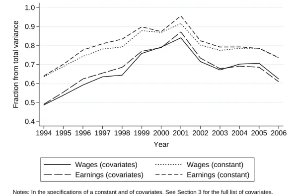
Figure 2 compares wage and earnings dynamics. It uses the parameter estimates from Table Figure 2: Evolution of the Fraction of the Permanent Variance Component, in specification
(S-AR) on the full sample
0.4 0.5 0.6 0.7 0.8 0.9 1.0
Fraction from total variance
1994 1995 1996 1997 1998 1999 2000 2001 2002 2003 2004 2005 2006 Year
Wages (covariates) Wages (constant)
Earnings (covariates) Earnings (constant)
Notes: In the specifications of a constant and of covariates. See Section 3 for the full list of covariates.
3 for the (S-AR) specification and shows the resulting fraction of permanent inequality (as a fraction from the total variance) for both wages and earnings. We can see that its evolution is virtually identical for earnings and wages in both variants, regressed on a constant and on the full set of covariates. Figure 6 in the Appendix depicts the corresponding results for the (S-ARMA) specification.
So far, all models predict an increase in the fraction of permanent inequality starting in 1994, a peak in 2000/2001 and a decline in subsequent years. While all specifications find this pattern, the exact level of permanent inequality depends on the underlying model. As a robustness check, we repeat the analysis on the subsample of only males. The results from these additional regressions, given graphically in Figures 7 and 8 in the Appendix, confirm our
findings.
Influence of Individual Characteristics
It becomes evident from Table 3 that controlling for individual characteristics leads to qual-itatively similar results as fitting just a constant. Most of the individual characteristics are time-invariant (gender or education) and it is essentially only age and possibly region which vary with time. The importance of controlling for individual characteristics thus primarily lies in accounting for changes in age (which proxies experience) and potentially for changing returns to these characteristics. It is of course not surprising that controlling for these factors reduces the level of dispersion. This follows simply from the fact that the fraction of explained variance from the first stage regression (Section 3) is larger. Figure 2 provides a direct comparison of the two sets of results. The variance after controlling for individual characteristics shrinks by about 20 percentage points. However, apart from this level effect, the same pattern emerges: rising relevance of permanent inequality from 1994 to 2000/2001, followed by a decline thereafter.
6 Concluding Remarks
There is by now a vast number of studies which document a sharp increase in cross-sectional wage inequality during the 2000s. It is often assumed that this inequality is of a “permanent nature” which in turn is sometimes used in policy discussions as an argument for a greater role of government regulation concerning the determination of wages and earnings. Applying longitudinal data on full-time working individuals in Germany from the GSOEP for the years of 1994 to 2006, we do not find unambiguous empirical support for this position.
By decomposing the cross-sectional variance into a permanent and a transitory part, we find that the fraction of permanent inequality in 2006 is greater compared to what it was in 1994. However this fraction is found to have declined by approximately 20 percentage points from 2001 to 2006, at the time of rapidly growing cross-sectional inequality. This implies that from about 2000 onward it is the year-to-year transitory volatility which becomes the increasingly important element of the growing cross-sectional inequality of wages and earnings in Germany.17
Our results are of course subject to a number of caveats. The analysis is by its nature limited to individuals who can be followed throughout the period we look at. This means that we do not take into account changes in wages of those who did not work at some point during the time 17Recent empirical evidence suggests that permanent inequality increased in the United States during the 2000s (Moffitt and Gottschalk, 2008). Thus, our results may indicate a new divergence between the United States and Germany during the 2000s in contrast to the increased convergence during the 1990s reported by Daly and Valletta (2008).
frame covered, as well as the new cohorts who came into the labour market since 1995. What reassures the validity of our conclusions is the fact that essentially the same results are obtained on a more restrictive sample excluding women. To further confirm the results obtained here one could consider dividing the analysis into several shorter periods or conducting it on other sub-samples of the population. This, however is left for future research.
References
Abowd, John M. and David Card, “On the Covariance Structure of Earnings and Hours
Changes,” Econometrica, March 1989, 57(2), 411–445.
Altonji, Joseph G. and Lewis M. Segal, “Small-sample Bias in GMM Estimation of
Co-variance Structures,” Journal Of Business & Economic Statistics, July 1996, 14(3), 353–366.
Bach, Stefan, Giacomo Corneo, and Viktor Steiner, “From Bottom to Top: The Entire
Distribution of Market Income in Germany, 1992-2001,” DIW Discussion Papers, 2007, 683.
, , and , “Effective Taxation of Top Incomes in Germany, 1992-2002,” DIW Discussion
Papers, 2008, 767.
Baker, Michael and Gary Solon, “Earnings Dynamics and Inequality among Canadian Men,
1976-1992: Evidence from Longitudinal Income Tax Records,” Journal of Labor Economics, April 2003, 21 (2), 289–321.
Biewen, Martin, “The Covariance Structure of East and West German Incomes and its
Implications for the Persistence of Poverty and Inequality,” German Economic Review, 2005,
6, 445–469.
Burkhauser, Richard V. and John G. Poupore, “A Cross-National Comparison of
Per-manent Inequality in the United States and Germany,” Review of Economics and Statistics, 1997, 79 (1), 10–17.
Burton, Peter and Shelly Phipps, “Families, Time and Money in Canada, Germany,
Swe-den, the United Kingdom and the United States,” Review Of Income And Wealth, September 2007, (3), 460–483.
Cappellari, Lorenzo, “The Dynamics and Inequality of Italian Male Earnings: Permanent
Changes of Transitory Fluctuations?,” ISER Working Paper 2000-41, Insitute for Social and Economic Research, University of Essex, 2000.
Chamberlain, Gary, “Panel Data,” in Michael D. Griliches, Zvi; Intriligator, ed., Handbook
of Econometrics, Vol. 2, Amsterdam: North-Holland, 1984, pp. 1247–1318.
Clark, Todd, “Small-sample Properties of Estimators of Nonlinear Models of Covariance
Struc-ture,” Journal of Business and Economic Statistics, 1996,14, 367–373.
Daly, Mary C. and Robert G. Valletta, “Cross-national Trends in Earnings Inequality and
Dickens, Richard, “The Evolution of Individual Male Earnings in Great Britain: 1979-95,”
The Economic Journal, 2000, 110, 27–49.
Dustmann, Christian, Johannes Ludsteck, and Uta Schönberg, “Revisiting the German
Wage Structure,” IZA Discussion Papers, 2007, 2685.
Gernandt, Johannes and Friedhelm Pfeiffer, “Rising Wage Inequality in Germany,”
SOEPpapers on Multidisciplinary Panel Data Research, 2007, 14.
Gustavsson, Magnus, “The 1990s Rise in Swedish Earnings Inequality - Persistent or
Tran-sitory?,” Applied Economics, January 2007, 39 (1), 25–30.
Haider, Steven J., “Earnings Instability and Earnings Inequality of Males in the United
States: 1967-1991,” Journal of Labor Economics, 2001, 19 (4), 799–836.
Haisken-DeNew, John P. and Joachim R. Frick, “Desktop Companion to the German
Socio-Economic Panel (SOEP) - Version 8.0,” Deutsches Institut für Wirtschaftsforschung (DIW), Berlin, 2005.
Lillard, Lee A. and Robert J. Willis, “Dynamic Aspects of Earnings Mobility,”
Economet-rica, 1978,46, 985–1012.
and Yoram Weiss, “Components of Variation in Panel Earnings Data - American Scientists
1960-70,” Econometrica, 1979, 47 (2), 437–454.
Maasoumi, Esfandiar and Mark Trede, “Comparing Income Mobility in Germany and
the United States Using Generalized Entropy Mobility Measures,” Review of Economics and Statistics, 2001, 83 (3), 551–559.
MaCurdy, Thomas E., “The Use of Time-Series Processes to Model the Error Structure of
Earnings in a Longitudinal Data-Analysis,” Journal of Econometrics, 1982,18 (1), 83–114.
Müller, Kai-Uwe and Viktor Steiner, “Would a Legal Minimum Wage Reduce Poverty? :
A Microsimulation Study for Germany,” Discussion Papers of DIW Berlin 791, DIW Berlin, German Institute for Economic Research 2008.
Moffitt, Robert A. and Peter Gottschalk, “Trends In The Transitory Variance Of Earnings
In The United States,” The Economic Journal, 2002, 112(478), 68–73.
and , “Trends in the Transitory Variance of Male Earnings in the U.S., 1970-2004,” 09 2008. Paper presented at Labor and Population Workshop, Department of Economics, Yale University.
Wagner, Gert G., Joachim R. Frick, and Jürgen Schupp, “The German Socio-Economic Panel Study (SOEP) - Scope, Evolution and Enhancements,” Schmollers Jahrbuch, 2007,127, 139–170.
Appendix - Figures
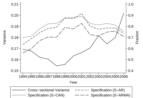
Figure 3: Cross-sectional Variance and its Permanent Component, for Wages in the specifica-tion with a constant on the full sample
0.4 0.5 0.6 0.7 0.8 0.9 1.0 Fraction 0.15 0.16 0.17 0.18 0.19 0.20 0.21 Variance 1994199519961997199819992000200120022003200420052006 Year
Cross−sectional Variance Specification (S−AR) Specification (S−CAN) Specification (S−ARMA)
Figure 4: Cross-sectional Variance and its Permanent Component, for Earnings in the speci-fication with covariates on the full sample
0.4 0.5 0.6 0.7 0.8 0.9 Fraction 0.09 0.10 0.11 0.12 0.13 0.14 0.15 Variance 1994199519961997199819992000200120022003200420052006 Year
Cross−sectional Variance Specification (S−AR) Specification (S−CAN) Specification (S−ARMA)
Notes: See Section 3 for the full list of covariates.
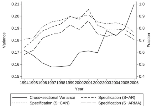
Figure 5: Cross-sectional Variance and its Permanent Component, for Earnings in the speci-fication with a constanton the full sample
0.4 0.5 0.6 0.7 0.8 0.9 1.0 Fraction 0.15 0.16 0.17 0.18 0.19 0.20 0.21 Variance 1994199519961997199819992000200120022003200420052006 Year
Cross−sectional Variance Specification (S−AR) Specification (S−CAN) Specification (S−ARMA)
Figure 6: Evolution of the Fraction of the Permanent Variance Component, in specification (S-ARMA) on the full sample
0.4 0.5 0.6 0.7 0.8 0.9 1.0
Fraction from total variance
1994 1995 1996 1997 1998 1999 2000 2001 2002 2003 2004 2005 2006 Year
Wages (covariates) Wages (constant) Earnings (covariates) Earnings (constant)
Notes: In the specifications of a constant and of covariates. See Section 3 for the full list of covariates.
Figure 7: Evolution of the Fraction of the Permanent Variance Component, in Specification (S-AR) on the reduced sample (male only)
0.4 0.6 0.8 1.0
Fraction from total variance
1994 1995 1996 1997 1998 1999 2000 2001 2002 2003 2004 2005 2006 Year
Wages (covariates) Wages (constant) Earnings (covariates) Earnings (constant)
Figure 8: Evolution of the Fraction of the Permanent Variance Component, in Specification (S-ARMA) on the reduced sample (male only)
0.2 0.4 0.6 0.8 1.0
Fraction from total variance
1994 1995 1996 1997 1998 1999 2000 2001 2002 2003 2004 2005 2006 Year
Wages (covariates) Wages (constant) Earnings (covariates) Earnings (constant)
Notes: In the specifications of a constant and of covariates. See Section 3 for the full list of covariates.
Table 4: Variance-Covariance Matrix -Earningsin the specification witha constant on the full sample
1994 1995 1996 1997 1998 1999 2000 2001 2002 2003 2004 2005 2006 1994 .1716 1995 .148 .1672 1996 .1341 .1425 .1611 1997 .1324 .1399 .1422 .1577 1998 .131 .136 .1398 .1421 .1581 1999 .129 .133 .1372 .1392 .1422 .159 2000 .1299 .1346 .1399 .1453 .1466 .1518 .17 2001 .1334 .138 .1423 .143 .1453 .1503 .1581 .1711 2002 .1227 .1278 .1346 .1352 .1379 .1428 .1489 .1532 .1696 2003 .1293 .1341 .1352 .1396 .1418 .1461 .1525 .1559 .156 .188 2004 .1255 .1312 .1333 .1357 .1397 .1457 .1512 .1555 .1536 .1677 .1838 2005 .124 .1306 .1351 .1385 .141 .1464 .1505 .1548 .1552 .1644 .1688 .19 2006 .1251 .1306 .1366 .1401 .143 .1493 .1542 .157 .1554 .1672 .1719 .1772 .2099
Notes: Number of observations for computing covariances is952.
Source: Own calculations using the GSOEP data (1994-2006).
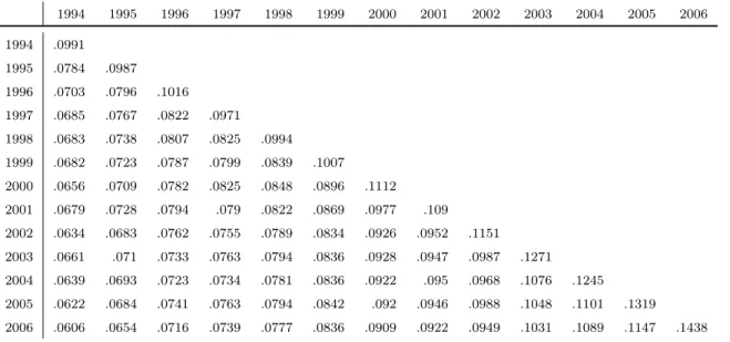
Table 5: Variance-Covariance Matrix -Earnings in the specification withcovariates on the full sample
1994 1995 1996 1997 1998 1999 2000 2001 2002 2003 2004 2005 2006 1994 .0991 1995 .0784 .0987 1996 .0703 .0796 .1016 1997 .0685 .0767 .0822 .0971 1998 .0683 .0738 .0807 .0825 .0994 1999 .0682 .0723 .0787 .0799 .0839 .1007 2000 .0656 .0709 .0782 .0825 .0848 .0896 .1112 2001 .0679 .0728 .0794 .079 .0822 .0869 .0977 .109 2002 .0634 .0683 .0762 .0755 .0789 .0834 .0926 .0952 .1151 2003 .0661 .071 .0733 .0763 .0794 .0836 .0928 .0947 .0987 .1271 2004 .0639 .0693 .0723 .0734 .0781 .0836 .0922 .095 .0968 .1076 .1245 2005 .0622 .0684 .0741 .0763 .0794 .0842 .092 .0946 .0988 .1048 .1101 .1319 2006 .0606 .0654 .0716 .0739 .0777 .0836 .0909 .0922 .0949 .1031 .1089 .1147 .1438
Notes: Number of observations for computing covariances is952. See Section 3 for the full list of covariates.
Table 6: Variance-Covariance Matrix - Wages in the specification with a constant on the full sample
1994 1995 1996 1997 1998 1999 2000 2001 2002 2003 2004 2005 2006 1994 .1694 1995 .1465 .1678 1996 .1303 .1381 .1621 1997 .1303 .1384 .139 .1605 1998 .1257 .1311 .1331 .1373 .1544 1999 .1263 .1287 .1313 .135 .1352 .1556 2000 .124 .1274 .1346 .1395 .1373 .145 .1633 2001 .128 .1323 .1369 .1387 .1362 .1415 .1497 .1664 2002 .1198 .1243 .1297 .1302 .1306 .1375 .1442 .1479 .1706 2003 .1234 .1291 .1279 .1339 .1317 .1382 .1446 .148 .15 .1816 2004 .1203 .1247 .1268 .1292 .1292 .1377 .1434 .1468 .1465 .1576 .1742 2005 .1199 .1246 .1285 .1325 .1307 .1379 .1423 .1471 .1505 .155 .1562 .18 2006 .1219 .1256 .1299 .1351 .1344 .1434 .147 .1492 .1513 .1582 .1599 .1639 .202
Notes: Number of observations for computing covariances is952.
Source: Own calculations using the GSOEP data (1994-2006).
Table 7: Variance-Covariance Matrix - Wages in the specification with covariates on the full sample
1994 1995 1996 1997 1998 1999 2000 2001 2002 2003 2004 2005 2006 1994 .0972 1995 .0774 .1002 1996 .0684 .0772 .1058 1997 .0688 .0778 .0831 .1049 1998 .0652 .0716 .0781 .0826 .1005 1999 .0671 .07 .0761 .0799 .0811 .1007 2000 .0624 .0666 .0771 .0819 .0808 .0873 .1083 2001 .0649 .0697 .0781 .0798 .0783 .0827 .0933 .1083 2002 .0622 .0667 .0744 .0747 .0759 .0816 .091 .0933 .1187 2003 .0635 .0695 .071 .0767 .0754 .0813 .09 .0921 .0971 .127 2004 .0634 .0676 .0721 .0741 .0749 .0821 .0905 .0926 .0952 .1047 .1231 2005 .0627 .0672 .0738 .0775 .0764 .0822 .0898 .0931 .0993 .1024 .1056 .1298 2006 .0615 .0647 .0707 .0758 .0759 .0838 .0897 .0907 .0962 .1013 .1051 .1096 .1444
Notes: Number of observations for computing covariances is952. See Section 3 for the full list of covariates.
Table 8: Variance-Covariance Matrix -Earningsin the specification witha constant on the reduced sample (male only)
1994 1995 1996 1997 1998 1999 2000 2001 2002 2003 2004 2005 2006 1994 .1606 1995 .1401 .1627 1996 .1268 .1387 .1612 1997 .125 .1346 .1386 .1558 1998 .1261 .1331 .1389 .1411 .1613 1999 .1242 .1295 .1364 .1378 .1428 .1617 2000 .1242 .1305 .1384 .1443 .1474 .1539 .1733 2001 .1281 .1336 .1401 .1402 .1452 .1514 .159 .1724 2002 .1151 .1208 .1314 .1303 .1365 .1416 .1475 .1516 .1698 2003 .1188 .1261 .1304 .1342 .1385 .1431 .1502 .1528 .151 .1828 2004 .1155 .1233 .1278 .1291 .1362 .1432 .1485 .1523 .1486 .162 .1808 2005 .1155 .1231 .1315 .1338 .1395 .1457 .1499 .1529 .1521 .1581 .1664 .1863 2006 .1143 .1201 .1303 .1328 .1403 .1474 .1529 .154 .1504 .162 .168 .1733 .1967
Notes: Number of observations for computing covariances is728.
Source: Own calculations using the GSOEP data (1994-2006).
Table 9: Variance-Covariance Matrix -Earnings in the specification withcovariates on the reduced sample (male only)
1994 1995 1996 1997 1998 1999 2000 2001 2002 2003 2004 2005 2006 1994 .0921 1995 .0717 .0936 1996 .0656 .0766 .1042 1997 .0625 .071 .08 .0951 1998 .0639 .07 .0805 .0807 .1011 1999 .063 .0672 .078 .0771 .0824 .1009 2000 .0604 .066 .0774 .0804 .0838 .0896 .1125 2001 .064 .0689 .0789 .0763 .0816 .0873 .0976 .1104 2002 .0576 .0625 .0749 .071 .0772 .0814 .0905 .0938 .1153 2003 .0578 .0644 .0709 .0715 .0761 .0803 .0901 .0921 .0944 .1232 2004 .056 .0626 .069 .0672 .0741 .0804 .0889 .0921 .0922 .1027 .1222 2005 .055 .0615 .0721 .0714 .077 .0824 .09 .0923 .0952 .0984 .1076 .1275 2006 .0522 .0564 .0675 .0671 .0749 .0815 .0895 .0901 .091 .0993 .1063 .1115 .1329
Notes: Number of observations for computing covariances is728. See Section 3 for the full list of covariates.
Table 10: Variance-Covariance Matrix - Wages in the specification with a constant on the reduced sample (male only)
1994 1995 1996 1997 1998 1999 2000 2001 2002 2003 2004 2005 2006 1994 .1623 1995 .1406 .1639 1996 .126 .1358 .1655 1997 .126 .1346 .1372 .1601 1998 .1225 .1285 .1323 .1356 .1576 1999 .125 .1268 .1322 .1354 .1371 .1617 2000 .1205 .1244 .1344 .1387 .1377 .1491 .1671 2001 .1238 .1284 .1354 .1358 .1349 .1433 .151 .1666 2002 .1141 .1176 .1272 .1242 .1283 .1375 .1437 .1453 .17 2003 .1154 .1219 .1238 .1277 .1273 .137 .143 .1435 .1441 .1769 2004 .1128 .1175 .1227 .1231 .1254 .1371 .1421 .1439 .1418 .1526 .1727 2005 .1139 .1182 .1268 .1287 .1284 .1392 .1429 .1459 .1475 .1488 .1538 .1774 2006 .114 .1167 .125 .129 .1312 .1441 .1477 .146 .1468 .1531 .1567 .1607 .1915
Notes: Number of observations for computing covariances is728.
Source: Own calculations using the GSOEP data (1994-2006).
Table 11: Variance-Covariance Matrix - Wages in the specification with covariates on the reduced sample (male only)
1994 1995 1996 1997 1998 1999 2000 2001 2002 2003 2004 2005 2006 1994 .0913 1995 .0704 .0937 1996 .0634 .0731 .1088 1997 .063 .0711 .0799 .102 1998 .0601 .0658 .0755 .0781 .1005 1999 .0629 .0644 .0745 .0766 .0789 .1021 2000 .0567 .0604 .0748 .0777 .0774 .087 .1077 2001 .0596 .064 .0757 .0749 .0744 .0817 .0913 .1066 2002 .0557 .0588 .071 .0669 .071 .0785 .0872 .0886 .1155 2003 .0553 .0614 .0665 .0688 .0689 .0776 .0854 .0857 .0894 .121 2004 .0557 .0596 .0677 .0665 .069 .079 .0867 .0883 .0888 .0985 .1208 2005 .0555 .0591 .0711 .0715 .0713 .0802 .0868 .0895 .0938 .0941 .1013 .1245 2006 .0535 .055 .0654 .0681 .0708 .0822 .0877 .0861 .0903 .0952 .1013 .1049 .1339
Notes: Number of observations for computing covariances is728. See Section 3 for the full list of covariates.
Table 12: Parameter Estimates - Reduced Sample (Male Only)
AR(1) ARMA(1,1)
Earnings Wages Earnings Wages constant covariates constant covariates constant covariates constant covariates
σ2 v0 0.080 0.060 0.084 0.062 0.046 0.033 0.056 0.035 (0.015) (0.014) (0.022) (0.020) (0.006) (0.005) (0.007) (0.005) σ2 µ 0.097 0.039 0.101 0.040 0.086 0.029 0.083 0.028 (0.002) (0.002) (0.003) (0.002) (0.004) (0.003) (0.005) (0.003) σ2 ε 0.029 0.025 0.034 0.031 0.038 0.034 0.039 0.036 (0.004) (0.004) (0.005) (0.004) (0.003) (0.002) (0.003) (0.002) ρ 0.652 0.655 0.590 0.574 0.868 0.897 0.867 0.880 (0.024) (0.024) (0.027) (0.027) (0.028) (0.015) (0.027) (0.022) γ -0.418 -0.437 -0.497 -0.494 (0.032) (0.020) (0.027) (0.022) p1995 1.046 1.077 1.030 1.052 1.041 1.062 1.040 1.060 (0.014) (0.030) (0.017) (0.033) (0.011) (0.027) (0.013) (0.028) p1996 1.099 1.231 1.071 1.205 1.113 1.263 1.100 1.245 (0.015) (0.033) (0.018) (0.037) (0.016) (0.043) (0.017) (0.040) p1997 1.111 1.198 1.085 1.203 1.121 1.193 1.113 1.228 (0.016) (0.034) (0.019) (0.038) (0.017) (0.046) (0.020) (0.045) p1998 1.153 1.283 1.085 1.207 1.158 1.266 1.105 1.206 (0.017) (0.037) (0.019) (0.040) (0.019) (0.054) (0.022) (0.051) p1999 1.205 1.376 1.172 1.357 1.219 1.395 1.225 1.427 (0.018) (0.040) (0.022) (0.045) (0.024) (0.066) (0.029) (0.060) p2000 1.242 1.495 1.193 1.434 1.231 1.377 1.227 1.453 (0.019) (0.045) (0.023) (0.048) (0.028) (0.084) (0.032) (0.081) p2001 1.322 1.661 1.213 1.454 1.377 1.633 1.263 1.553 (0.018) (0.043) (0.024) (0.051) (0.032) (0.115) (0.035) (0.079) p2002 1.176 1.433 1.132 1.373 1.160 1.354 1.165 1.409 (0.019) (0.044) (0.021) (0.046) (0.025) (0.077) (0.031) (0.077) p2003 1.203 1.427 1.142 1.367 1.196 1.358 1.187 1.413 (0.018) (0.043) (0.021) (0.045) (0.025) (0.078) (0.032) (0.080) p2004 1.192 1.420 1.135 1.400 1.203 1.416 1.206 1.529 (0.018) (0.041) (0.020) (0.045) (0.024) (0.079) (0.032) (0.082) p2005 1.217 1.466 1.168 1.456 1.243 1.527 1.263 1.662 (0.018) (0.041) (0.020) (0.046) (0.024) (0.084) (0.035) (0.092) p2006 1.232 1.446 1.193 1.449 1.257 1.478 1.285 1.611 (0.017) (0.040) (0.020) (0.044) (0.024) (0.080) (0.034) (0.082) λ1996 0.875 0.959 0.932 1.008 0.859 0.938 0.941 1.015 (0.062) (0.070) (0.074) (0.078) (0.034) (0.034) (0.034) (0.033) λ1997 0.822 0.918 0.873 0.957 0.818 0.908 0.921 0.990 (0.070) (0.077) (0.080) (0.083) (0.039) (0.036) (0.041) (0.038) λ1998 0.778 0.892 0.844 0.934 0.805 0.907 0.927 0.991 (0.075) (0.082) (0.083) (0.085) (0.044) (0.041) (0.045) (0.041) λ1999 0.574 0.731 0.603 0.728 0.676 0.804 0.754 0.858 (0.089) (0.087) (0.102) (0.094) (0.057) (0.053) (0.062) (0.051) λ2000 0.647 0.699 0.646 0.692 0.769 0.909 0.818 0.886 (0.088) (0.097) (0.102) (0.109) (0.062) (0.055) (0.065) (0.060) λ2001 -0.076 -0.046 0.485 0.593 0.316 0.679 0.745 0.794 (0.103) (0.114) (0.124) (0.115) (0.140) (0.097) (0.070) (0.065) λ2002 0.791 0.835 0.850 0.881 0.866 0.935 0.961 0.985 (0.077) (0.087) (0.085) (0.090) (0.049) (0.047) (0.050) (0.048) λ2003 0.882 0.956 0.906 0.965 0.921 0.998 0.993 1.036 (0.076) (0.086) (0.084) (0.089) (0.048) (0.046) (0.050) (0.047) λ2004 0.916 0.980 0.900 0.940 0.909 0.966 0.937 0.962 (0.076) (0.087) (0.084) (0.089) (0.048) (0.046) (0.050) (0.048) λ2005 0.910 0.978 0.858 0.897 0.886 0.932 0.873 0.882 (0.076) (0.087) (0.084) (0.089) (0.049) (0.046) (0.053) (0.054) λ2006 1.007 1.090 0.969 1.035 0.953 1.010 0.964 1.014 (0.079) (0.091) (0.085) (0.089) (0.051) (0.046) (0.053) (0.049) N 91 91 91 91 91 91 91 91
Notes: See Section 3 for the full list of covariates.