Socially-Efficient Tax Reforms

Socially-Efficient Tax Reforms

∗

Jean-Yves Duclos

, Paul Makdissi

and Quentin Wodon

February 2002

Abstract

We propose graphical methods to determine whether commodity-tax changes are “socially efficient”, in the sense of improving social welfare or decreasing poverty for large classes of social welfare and poverty indices. We also derive estimators of critical poverty lines and economic efficiency ratios which can be used to characterize socially-efficient tax reforms. The statistical properties of the various estimators are derived in order to make the method implementable using survey data. The methodology is illustrated using a recently-proposed reform of the Mexican Valued Added Tax system.

Keywords: Social welfare, Poverty, Efficiency, Tax Reform, Stochastic Dominance JEL Numbers: D12, D63, H21, I32

∗ _{We thank R. Alessie, J.O. Lanjouw, P. Lanjouw, M. Ravallion, S. Yitzhaki for many useful}

com-ments. This paper was funded through the World Bank Research Support Budget under the research project “The impact of changes in prices, taxes, subsidies and stipends on poverty when households differ in needs” and has also benefitted from the support of SSHRC, the MIMAP programme of IDRC and Bureau de la recherche of Universit´e de Sherbrooke.

† _{CR´EFA, Universit´e Laval, Qu´ebec, and Institut d’An`alisi Econ`omica, CSIC, Barcelona.}

Corre-sponding address: CR´EFA, D´epartement d’´economique, Pavillon De S`eve, Universit´e Laval, Sainte-Foy, Qu´ebec, Canada, G1K 7P4. Email: [email protected]

‡ _{D´epartement d’´economique and CEREF, Universit´e de Sherbrooke, 2550 boulevard de l’Universit´e,}

Sherbrooke, Qu´ebec, Canada, J1K 2R1; email: [email protected]

§ _{LCSPR, World Bank, 1818 H Street, NW, Washington, DC 20433, USA, Email:}

1

Introduction

Policies that affect consumer and producer prices have an impact on welfare, and there are many such policies. Some governments maintain high import tariffs or fail to im-plement regulations to foster competition. This may protect national producers by maintaining high domestic producer prices, but it also raises consumption prices, which hurts consumers. Most governments use sales and indirect taxes to raise tax revenues, thus affecting consumer and producer prices. This is particularly important for develop-ing countries, which rely heavily on commodity taxation to generate tax revenues. Price subsidies on food, education, energy and transportation are also common in developing and developed countries alike.

Policy analysts must routinely evaluate the impact of such pricing policies on poverty and social welfare. Important information problems stand, however, in the way of any-one wishing to do this. The main objective of the paper is to show how these problems can be (somewhat) circumscribed. We are particularly interested in demonstrating the empirical applicability of a “social efficiency” approach, which makes it possible to iden-tify price changes that will be deemed socially desirable by wide spectra of social welfare and poverty analysts. For expositional simplicity, we will focus in this paper on the analysis of the effect of indirect tax reforms on social welfare and poverty. We will think of two goods,j andl, and will ask whether it is socially desirable (in a sense to be defined precisely below) to increase a tax rate on goodj in order to decrease a tax rate on good

l. Note that tax rates may be positive or negative, which also says that decreasing the tax on a good may mean increasing its rate of subsidy. In doing this, we keep producer prices constant for expositional simplicity, but this framework can be extended to the general equilibrium analysis of any government intervention that changes relative prices. The first measurement difficulty is then to estimate the impact of price changes on consumer welfare. It is well known that this can be a complicated exercise and that its results can be sensitive to a number of important theoretical and econometric assump-tions. The task is particularly problematic when the goal is to find globally optimal tax systems, since the tax analyst then needs reliable demand responses over extended price intervals for each household. Keeping in mind that actual changes in the tax system are “slow and piecemeal” ( see for instance Feldstein (1975)), and that it would be unwise to ignore the role of the actual tax system as a departure (or anchor) point for the identifi-cation of desirable tax reforms, we focus here on the effect of marginal tax reforms. One immediate advantage is that evaluating the distributive impact of marginal tax reforms does not require estimates of individual demand and utility functions, but can instead be assessed directly from the observed data alone1_{, as we review in Section 2.}

The second difficulty resides in the choice of a social evaluation function with which the impact of the tax reform is to be measured2_{. This choice poses a fundamental} problem, since any particular selection of functional form and parameters for a social evaluation function necessarily embodies arbitrary value judgements. The strategy we follow in this paper is instead to define classes of social evaluation indices that incorporate increasingly stronger judgements on the importance of distributive issues in designing tax policy. For this purpose, we consider social evaluation indices that take into account (though not necessarily with the same distributive weight) everyone’s welfare – the traditional social welfare functions – as well as social evaluation indices that censor welfare at a poverty line and which are therefore not affected by changes in the welfare of the “rich” – in short, the much-used poverty indices. These classes of functions and indices are described in Section 3.

Verifying whether a tax reform is desirable then proceeds by checking whether it can command the unanimous approval of all those analysts who agree with some generally-defined normative properties of the social evaluation indices. If so, the reform can be called “socially efficient”. One well-known criterion for social efficiency property comes from the Pareto principle. Pareto efficiency, however, is likely to provide a poor norma-tive basis for the empirical analysis of tax reforms (for reasons that we discuss below in Section 7), and it is thus useful to consider “higher-order” ethical principles. We increase progressively the ethical content of our classes of social welfare and poverty indices by incorporating the anonymity – or symmetry – principle (for first-order efficiency), the Pigou-Dalton principle of transfers (for second-order efficiency), the principle of dimin-ishing transfers (for third-order efficiency), and subsequent “generalized” higher-order normative principles. These principles lead to the definition of what we term Pen-efficient, Dalton-Pen-efficient, Kolm-efficient and higher-order welfare-efficient tax reforms. The definition of poverty-efficient tax reforms proceeds in a similar way by censoring the social assessment at a poverty line. This is derived in Section 4.

The third difficulty lies in estimating the impact on tax revenues of changes in the structure of indirect taxation. It is well known that this impact is linked to the aggregate deadweight loss of taxation (Wildasin (1984) and Mayshar (1990)), and thus to the economic efficiency of a tax reform. Estimating the aggregate impact on tax revenues can be less difficult (in principle at least) than the estimation of household-specific changes in consumption, but the details of the estimation procedures can still lead to Ahmad and Stern (1984, 1991), Besley and Kanbur (1988), Yitzhaki and Thirsk (1990), Yitzhaki and Slemrod (1991), Mayshar and Yitzhaki (1995), Yitzhaki and Lewis (1996) and Makdissi and Wodon (2002).

2_{See Deaton (1977), King (1983) and Besley and Kanbur (1988) for examples of the use of particular}

social evaluation functions in assessing tax reforms, and Christiansen and Jansen (1978) and Ahmad and Stern (1984) for the estimation of “implicit social preferences”.

considerable disagreements among tax analysts. One solution is to carry out sensitivity analysis on the role of the unobserved economic efficiency parameter, in the manner of Ahmad and Stern (1984) for instance. We propose an alternative procedure that estimates the critical efficiency ratio up to which a tax reform can be said to be socially efficient at a given ethical order. This leaves policy makers free to assess whether the actual efficiency ratio is likely (or can be safely estimated) to be below that critical value, and thus whether the tax reform can confidently be deemed socially efficient. A similar device is constructed to handle, for poverty measurement, the role of poverty lines – whose estimation is also notoriously difficult and controversial. We show how to construct estimates of the critical poverty lines up to which a tax reform can be considered to be poverty efficient. Policy makers and poverty analysts are then let free to assess or estimate whether those critical poverty lines are sufficiently high to encompass all plausible poverty line estimates. If that is so, the tax reform can be confidently described as poverty efficient. These critical thresholds are derived in Section 5.

Social efficiency is checked in this paper through the use of simple Consumption Dominance (CD) curves. CD curves display cumulative consumption shares when these are weighted by powers of poverty gaps. First-order CD curves show the share in the total consumption of a good of those at a given income level. Second-order CD curves indicate the combined share in the total consumption of a good of those whose income lies below a given threshold. Higher-order CD curves weight consumption shares by increasingly higher powers of poverty gaps. Increasing the tax on goodj and decreasing the tax on good l is poverty efficient at any given order of ethical dominance if the

CD curve of that order for good l is higher than the CD curve for good j at every threshold under a maximum poverty line. When that maximum poverty line extends to infinity, the tax reform can be called welfare efficient. The second-order welfare efficiency condition we obtain is equivalent to the Dalton efficiency condition of Yitzhaki and Slemrod (1991) and Mayshar and Yitzhaki (1995). Our social efficiency conditions become less stringent when we consider poverty instead of welfare efficiency, since we can then focus exclusively on those below a maximum admissible poverty line and do not need to consider the impact of the reform on the entire population. Increasing the order of dominance also facilitates the search for socially efficient tax reforms since more ethical structure is then imposed on the properties of the admissible social evaluation indices. These links are described in some detail in Section 6.

CD curves were first used by Makdissi and Wodon (2002) in the context of poverty reduction. This paper uses them for the broader analysis of social efficiency. The current paper also introduces the concept of first-order social efficiency and shows how to test it, and also discusses how it differs from the traditional concept of Pareto efficiency. The concept of social efficiency further leads to an interpretation of the ratio of CD curves as a natural indicator of the distributive benefit of a tax reform, a benefit which can

be compared to the deadweight loss or economic efficiency cost of the reform. We also see how the concepts of critical economic efficiency ratios and critical poverty lines may help circumvent some of the difficulties faced by tax analysts.

Tax policy analysis is clearly of practical and policy interest, and it is thus essential to consider how the tools described above can be implemented empirically using survey data. We do this in part in this paper by investigating in Section 8 the sampling prop-erties of estimators of CD curves, critical poverty lines and critical economic efficiency thresholds. In this, we make use inter alia of non-parametric regression curves for the analysis of first-order-efficient tax reforms.

The paper’s tools are applied in Section 9 to the analysis of a recent proposal for the reform of the Mexican Value-Added-Tax system. Section 10 concludes the paper, and the proofs of the various lemmas and theorems can be found in the Appendix.

2

Notation and definitions

Consider a vector qof K consumer prices. For expositional simplicity, and as is custom-ary in the partial equilibrium literature, we set the vector of producer prices to 1 and assume them to be constant and invariant to changes in t, the vector of K tax rates. We then have q = 1 +t and dqk =dtk, where qk and tk denote respectively the price of and the tax rate on good k.

Let y be exogenous nominal income, and denote consumers’ preferences by θ. The indirect utility function is given by v(y, θ, q). Following King (1983), we will be using a vector of reference prices, qR_{, to assess consumers’ well-being in the presence of varying} tax rates. Denote the real (or equivalent) income in the post-reform situation by yR_, whereyR_{is measured on the basis of the reference prices q}R_{. y}R _{is implicitly defined by}

v¡yR_{, θ, q}R¢ _{=v(y, θ, q), and explicitly by the real income function y}R_{= ρ}¡_{y, θ, q, q}R¢_, where

v¡ρ¡y, θ, q, qR¢_{, θ, q}R¢_{≡v(y, θ, q). (1)} By definition, yR _{gives the level of income that provides under q}R _{the same utility as}

y yields under q. The nominal income function, y = η¡yR_{, θ, q, q}R¢_{, is the inverse of}

ρ¡y, θ, q, qR¢ _{and is such that}

v¡yR_{, θ, q}R¢_≡v¡_η¡_yR_{, θ, q, q}R¢_{, θ, q}¢_{. (2)} The nominal income function gives the level of income that yields the same utility under

We then wish to determine how consumer welfare is affected by a marginal change in tax rates. Letxk(y, θ, q) be the net consumption of goodk of a consumer with incomey, preferencesθ and facing pricesq. xk(y, θ, q) can be negative if there are net producers of

k in the economy. Using Roy’s identity and setting reference prices to pre-reform prices, we find: ∂ρ(y, θ, q, qR₎ ∂tk ¯ ¯ ¯ ¯ q=qR = ∂v(y, θ, q)/∂tk ∂v(yR_{, θ, q}R_)/∂yR ¯ ¯ ¯ ¯ q=qR = − ∂v(y, θ, q)/∂y ∂v(yR_{, θ, q}R_)/∂yR ¯ ¯ ¯ ¯ q=qR ·xk(y, θ, q) = −xk ¡ y, θ, qR¢. (3) Similarly, ∂η¡yR_{, θ, q, q}R¢ ∂tk ¯ ¯ ¯ ¯ ¯ q=qR =xk ¡ y, θ, qR¢_{. (4)} Equations (3) and (4) say that observed pre-reform consumption of goodkis a sufficient statistic to know the impact on consumer welfare of a marginal change in the price of good k 3_.

Assume that preferences θ and exogenous income yare jointly distributed according to the distribution functionF(y, θ). The conditional distribution ofθ givenyis denoted byF(θ|y), and the marginal distribution of nominal income is given byF(y). Continuity across y of the conditional distribution function F(θ|y) is not generally needed for the methodological results of this paper, but empirical applicability of some of these results will sometimes require such a continuity assumption, as we will discuss explicitly in Section 8. Let preferences belong to the set Ω, and assume income to be distributed over [0, a]. Expected consumption of good k at income y is then given by xk(y, q):

xk(y, q) =E

θ [xk(y, θ, q)] = Z

Ω

xk(y, θ, q)dF(θ|y). (5) Let Xk(q) then be the per capita consumption of the kth good, defined as Xk(q) = R_a

0 xk(y, q) dF (y). By (3) and (4),Xk(q) is also the average welfare cost of an increase in the price of good k.We will often normalize by Xk(q) some of the various measures that will be associated to a good k, and we will distinguish these normalized measures

with a ·. Hence, as a proportion of per capita consumption, consumption of good k at incomey is expressed asxk(y, q) = xk(y, q)/Xk(q).

We now turn to the government budget constraint. Per capita commodity tax rev-enues, R(q), equal R(q) = P_kK₌₁tkXk(q). Without loss of generality, assume that the government’s marginal tax reform increases the tax rate on thejth _{commodity and uses} the proceeds to decrease the tax rate (or to increase the subsidy) on the lth commod-ity. As is conventional in the optimal taxation literature, total tax revenues are kept invariant to the tax reform. Revenue neutrality of the tax reform requires that

dR(q) = " Xj(q) + K X k=1 tk ∂Xk(q) ∂qj # dqj+ " Xl(q) + K X k=1 tk ∂Xk(q) ∂ql # dql = 0. (6) Defineγ as γ = Xl+ P_K k=1tk∂X∂qlk Xl , Xj + P_K k=1tk∂X∂qjk Xj , (7)

where, for expositional simplicity, the (q)’s have been omitted. The numerator in (7) gives the marginal tax revenue of a marginal increase in the price of good l, per unit of the average welfare cost that this price increase imposes on consumers. Equivalently, this is 1 minus the deadweight loss of taxing good l, or the inverse of the marginal cost of public funds (MCPF) from taxing l (see Wildasin (1984)). The denominator gives exactly the same measures for an increase in the price of good j. γ is thus the economic (or “average”) efficiency of taxing good l relative to taxing good j. We may thus interpret γ as the efficiency cost of taxing j relative to that of taxing l (the MCPF for j over that for l). The higher the value of γ, the less economically efficient is taxing good j.

By simple algebraic manipulation, we can then rewrite equation (6) as

dqj =−γ µ Xl Xj ¶ dql, (8)

which fixes dqj as a revenue-neutral proportion of dql.

3

Measuring poverty and social welfare

To assess the impact of a tax reform on poverty and social welfare, we follow the main custom in the measurement literature and focus for simplicity on additive poverty and

social welfare indices. For first, second and third order dominance, this is only to ease the necessity and sufficiency proofs of the various social efficiency conditions: we could use some of the results of the previous literature to show that the relevant classes of indices also include subclasses of non-additive indices as well4_{. This additivity assumption is} such poverty indices can be expressed as:

P (z) = Z _a

0

p(y, z)dF (y) (9) where P (z) is an additive poverty index, z is the poverty line defined in income space and p(y, z) is the contribution to total poverty of a consumer with income y (with

p(y, z) = 0 for all y > z)5_.

For the poverty efficiency results of this paper, we consider the classes of poverty indices P(z)∈Πs _{defined such that}

Πs_{(z) =}   P(z) ¯ ¯ ¯ ¯ ¯ ¯ p(y, z) = 0 if y > z, p(y, z)∈Cbs_(z), (−1)ip(i)_{(y, z)≥0 fori= 0,1, ..., s,} p(t)_{(z, z) = 0 for t= 0,1, ..., s−2 whens≥2}    (10)

where Cbs_{(z) is the set of functions that are s-time piecewise differentiable}6 _{over [0, z],} and where the subscript(s) _{stands for ans}th_{-order derivative with respect toy. We will} return very shortly to the interpretation of the derivative assumptions.

A particular subclass of additive poverty indices to which we will make repeated references below is found in Foster, Greer and Thorbecke (1984) and is defined forα≥0 by F GTα_{(z) =} Z _z 0 µ z−y z ¶_α dF (y). (11)

4_{See, for instance, Dasgupta, Sen and Starrett (1973) and Foster and Shorrocks (1988a,b).}

5_{It is best in this section to think of y and z as real variables. Defining the poverty line in the}

real income space rather than in the nominal income space is convenient since the poverty line is then invariant to tax reforms. In this paper, as mentioned above, we generally suppose that pre-reform nominal and real incomes are initially the same since we take reference prices as the pre-reform prices (this is the common – though arbitrarily-made – assumption in the literature; see Donaldson (1992) for a general discussion). In any case, the marginal distribution of real income,FR(yR),can always be computed from the joint distribution of nominal income and preferencesF(y, θ):

FR(yR) = Z Ω Z _η(yR_,θ,Q) 0 dF(y, θ).

6_{When the (s−1)}th _{derivative is a piecewise differentiable function, the function and its (s−2)} first derivatives are differentiable everywhere. TheCbs_{(z) continuity assumption is made for analytical} simplicity since it could be relaxed to include indices whose (s−1)th _{derivative is discontinuous (and} which are therefore nots-time piecewise differentiable).

F GT0_{(z) gives the most widely used index of poverty, the so-called poverty headcount,} and F GT1_{(z) yields the second most popular index, the (normalized) average poverty} gap. Note that F GTα_{(z) belongs to Π}s_{(z) for α ≥ s −1. The FGT indices were in} fact used by Besley and Kanbur (1988) for their analysis of price subsidies (thus in fact supposing an explicit form for p(y, z)). Other well-known additive indices that also belong to Π1_{(z) and Π}2_{(z) include the Watts (1968) index, the second class of indices} proposed by Clark, Hemming and Ulph (1981), and the class of indices proposed by Chakravarty (1983).7

Turning now to social welfare, we consider utilitarian social welfare functions U such that:

U = Z _a

0

u(y)dF (y). (12) We focus on social welfare indices that belong to the classes Ωs_{, s = 1,2, . . .. They are} defined as

Ωs₌n_U¯¯_¯u(y)∈Cs_(∞),(−1)i+1_u(i)_{(y)≥0 fori= 1,2, ..., s,}o_{. (13)} It is useful at this point to provide a normative interpretation of the different classes of indices of poverty and social welfare. When s = 1, poverty indices weakly decrease (p(1)_{(y, z)≤0) while welfare indices weakly increase (u}(1)_{(y)≥0) when an individual’s} income increases. These indices are thus Paretian but they also obey the well-known symmetry or anonymity axiom: interchanging any two individuals’ incomes leaves un-changed the poverty and social welfare indices. Ordering two distributions of living standards over the first-order classes of indices is equivalent to making the living stan-dards “parade” simultaneously alongside each other, and verifying if one parade weakly dominates the other (this exercise was first suggested by Pen (1971, ch.III)). For poverty comparisons, the distributions of living standards are simply censored at z. For simplic-ity, we will refer to first-order welfare-efficient tax reforms as “Pen-efficient tax reforms”. When s = 2, poverty indices are convex and welfare indices are concave. They must thus respect the Pigou-Dalton principle of transfers, which postulates that a mean-preserving transfer of income from a higher-income person to a lower-income person constitutes a social improvement, in the form of increasing social welfare or decreasing poverty. We follow the lead of Mayshar and Yitzhaki (1995) by denoting as “Dalton-efficient tax reforms” those reforms that will be found to be second-order welfare “Dalton-efficient. By their third-order derivative, the poverty and social welfare indices that belong to Π3 _{and Ω}3 _{must also be sensitive to favorable composite transfers. These transfers are}

7_{As pointed out in Zheng (1999), it is possible to transform some of those indices in order to make}

them satisfy higher-order conditions. Relaxing the additivity or piecewise differentiability assumptions would also include other indices in the Πs_{(z) classes.}

such that a beneficial Pigou-Dalton transfer within the lower part of the distribution, accompanied by an adverse Pigou-Dalton transfer within the upper part of the distri-bution, will add to social welfare, provided that the variance of the distribution is not increased. Kolm (1976) was the first to introduce this condition into the inequality lit-erature, and we therefore refer for simplicity to third-order welfare efficient tax reforms as “Kolm-efficient tax reforms”. Kakwani (1980) subsequently adapted this principle to poverty measurement8_.

For the interpretation of higher orders of dominance, we can use the generalized transfer principles of Fishburn and Willig (1984). For s = 4, for instance, consider a combination of two exactly opposite and symmetric composite transfers, the first one being favorable and occurring within the lower part of the distribution, and the second one being unfavorable and occurring within the higher part of the distribution. Because the favorable composite transfer occurs lower down in the income distribution, indices that are members of the s = 4 classes will respond favorably to this combination of composite transfers. Generalized higher-order transfer principles essentially postulate that, assincreases, the weight assigned to the effect of transfers occurring at the bottom of the distribution also increases. Blackorby and Donaldson (1978) describe these indices as becoming more Rawlsian. Thus, as shown in Davidson and Duclos (2000) for poverty indices, when s → ∞ only the lowest income counts, although this result does not generalize to welfare dominance, as shown in Duclos and Makdissi (2000) and as will also appear later.

4

Identifying Socially Efficient Tax Reforms

To derive the conditions by which the social efficiency of tax reforms can be checked, it is handy first to refer to stochastic dominance curves. In real income space, these are defined as Ds_{(z) =} 1 (s−1)! Z Ω Z _η(z,θ,Q) 0 [z−ρ(y, θ, Q)](s−1)dF (y, θ), (14) for orders of dominance s = 1,2, ... When q = qR_{, we have that z = η}¡_{z, θ, q, q}R¢ ₌

ρ¡z, θ, q, qR¢_{, and (14) then reduces to the simpler expression}

Ds_{(z) =} 1 (s−1)!

Z _z 0

[z−y](s−1)dF (y). (15)

8_{See also Shorrocks and Foster (1987) for a characterization of the composite transfer principle and}

Dominance curves are therefore just sums of powers of poverty gaps. They can thus be interpreted as ethically-weighted sums of individual deprivation. The larger the value ofs, the larger the weights on the largest poverty gaps. Clearly, as can be seen by comparing (11) and (15), dominance curves have a convenient link with the FGT indices since F GTα_{(z) = (α)!z}−α_Dα+1_(z).

It is thus useful to consider how the dominance curves are affected by changes in prices. By (3), (4) and (14), we can show that:

∂Ds_(z) ∂tk ¯ ¯ ¯ ¯ q=qR = ½ xk ¡ z, qR¢ _{f(z), ifs= 1} 1 (s−2)! R_z 0 xk ¡ y, qR¢ _(z−y)s−2 _{dF (y) ifs= 2,3, ...} (16) wheref(z) is the density of income atz. For reasons that will become clear later, these derivatives can serve to define “consumption dominance” (CD) curves:

CDs k(z) = ∂Ds_(z) ∂tk , s= 1,2, ... (17) BecauseCDs

k(z) curves describe changes in ethically weighted sums of deprivation, they can be interpreted as the ethically weighted cost of taxing k. Normalized CD curves,

CDs_k(z), are just the above CD curves for good k normalized by the average consump-tion of that good:

CDs_k(z) = CDks(z)

Xk(q)

. (18)

CD curves are thus the ethically weighted (or social) cost of taxing k as a proportion of the average welfare cost. Note that the social cost depends on s and z. By (16),

CD1_k(z) only takes account of the consumption pattern of those precisely at z. The

CD2_k(z) curve gives the share in the total consumption of k of those individuals with income less than z. For s = 3,4, ..., greater weight is given to the shares of those with higher poverty gaps. For z < a, the pattern of consumption and the welfare cost for some may be ignored in the computation of the social cost of taxing k. The social and average welfare cost coincide only when s= 2 and z ≥a, since we have CD2_k(z) = 1 for allz ≥a and all k.

Define a distribution function for the consumption of good k as

Gk(y) = Z _y

0

x(u, q)f(u)du. (19)

Gk(y) is the proportion of the total consumption of good k that is consumed by those with incomes less than y. Note that Gk(a) = 1. Fors≥2, it follows from (16) that

CDs_k(z) = 1 (s−2)! z Z 0 (z−y)s−2 dGk(y). (20) Hence, the CDs curves are scaled F GTα _{indices, using α = s−2 and a transformed} income distributionGk that weights individuals by their share in the total consumption of the good k. When multiplied by (s−1)!/zs−1_{, the CD curves for s = α + 1 have} the convenient feature of providing the impact on the F GTα_{(z) indices of a marginal} increase in the price of good k. This is important in its own right given the popularity of the FGT class of poverty indices.

Most importantly it would seem, Consumption Dominance curves can be used to test the poverty and welfare efficiency of tax reforms. This is shown in Theorems 1 and 2, where γ is defined as in (7).

Theorem 1 A necessary and sufficient condition for a revenue-neutral marginal tax reform, dqj = −γ

³ Xl Xj

´

dql > 0, to be s-order poverty efficient, that is, to decrease poverty weakly for all P(z) ∈Πs_{(z), for all z ∈ [0, z}+_{] and for a given s ∈ {1,2,3, ...},}

is that

CDs_l(y)−γCDs_j(y)≥0, ∀y∈£0, z+¤_{. (21)}

Proof. See appendix.

Theorem 1 is similar to the result obtained in Makdissi and Wodon (2000), except for the case of first-order poverty efficiency, which they did not consider. For welfare dominance, a similar theorem applies.

Theorem 2 A sufficient condition for a revenue-neutral marginal tax reform, dqj =

−γ

³ Xl Xj

´

dql >0, to bes-order welfare efficient, that is, to increase social welfare weakly for all W ∈Ωs _{and for a given s∈ {1,2,3, ...}, is that}

CDs_l(y)−γCDs_j(y)≥0, ∀y∈[0,∞). (22)

Proof. See appendix.

The only difference between the social efficiency conditions of Theorems 1 and 2 is that the social welfare test extends over the entire space [0,∞), while for poverty the test is limited to the range of potential poverty lines [0, z+_{]. For γ = 1, Theorem 1} says that the tax reform will reduce poverty in an ethically robust manner if the CD

curve of good l is higher than the CD curve of good j for every poverty line under z+_. When the range of poverty lines is unbounded, Theorem 2 extends such social efficiency to (global) welfare efficiency. For γ 6= 1, one simply translates the CD curve of good

j by the economic efficiency parameter γ before checking again the ordering of the CD

curves up to the maximum poverty line. Ethical robustness of poverty reduction implies that poverty will be reduced by the tax reform for all choices of poverty indices within Πs_{(z) and for all choices of poverty lines within [0, z}+_{]. Ethical robustness of welfare} increase means that social welfare will be increased by the tax reform for all choices of social welfare functions in Ωs_{. A tax reform is Pen efficient, Dalton efficient and Kolm} efficient if (22) holds for s= 1,2 or 3 respectively.

5

Critical poverty lines and efficiency ratios

The ratio CDs_l(z)/CDs_j(z) of normalized consumption dominance curves can be inter-preted as the distributive benefit of taxing j instead of l. To see why, assume again an increase in the tax on good j and thus a fall in the price of good l. The socially-weighted gain from this fall in ql, as a proportion of the average welfare gain, is given by CDs_l(z), which is therefore an indicator of the distributive benefit of taxing j. The same naturally holds for the distributive benefit of taxing l, which is given by CDs_j(z). Denote this distributive benefit ratio as δs(z) = CDs_l(z)/CDs_j(z). If CDs_j(z) = 0, the relative distributive benefit of taxingj is then effectively infinite, but for tractability we will then define it as γ++_{, which we may set to as large a finite value as we wish. δ}s_(z) is thus given by:

δs_{(z) =} ½CDsl(z) CDsj(z) if CD s j(z)6= 0, γ++ _{if CD}s j(z) = 0. (23) Note that δ1(z) is a normalized ratio of Engel curves at incomez. More precisely, it is the ratio, atz, of the share of good l over the share of goodj, divided by the ratio of the average shares over the entire population.

Thus, δs_{(z) is the distributive benefit of taxing j relative to that of taxing l. Recall} thatγ is the economic cost of taxingjrelative to that of taxingl. Comparing distributive benefit δs(z) to economic cost γ is crucial in determining whether a tax reform that increases tj and decreases tl is socially efficient. We can indeed re-write the conditions of Theorems 1 and 2 by checking whether δs(z) ≥ γ for all z ∈ [0, z+_{] and for all}

z ∈ [0,∞) (equations (21) and (22)), respectively. In words, a tax reform is s-order socially efficient if its distributive benefit exceeds its economic cost over a range of

alternative poverty lines. Note that when preferences are identical and homothetic, then by (19) Gj(y) = Gl(y) for all y, and therefore δs(z) = 1 whatever the values of

z and s. There is then no distributive benefit to the tax reform whatever the social welfare or poverty objectives. The optimal tax system is then one in which the marginal deadweight loss of taxation is the same across the two goods.

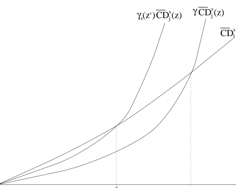
For a given value of γ = γ+_{, we assume from now onwards that – for some z}+ _and without loss of generality – we have that

CDs_l (z)−γCDs_j(z)≥0, for all z ∈[0, z+], (24) with strict inequality over at least part of the range. Such curves CDs_l(z) andγCDs_j(z) are shown on Figure 1. Condition (24) is clearly also valid for all other values ofγ < γ+_. Hence, either (24) also holds for all superior values ofγ > γ+_{, in which case we must have} that δs_{(z) = γ}++ _{for all z ∈ [0, z}+_{]. Or, there exists a critical value of γ beyond which} (24) does not hold everywhere over [0, z+_{]. Denoting this critical economic efficiency} threshold as γ_s(z+_{), we have:}

γ_s(z+_{) = inf}©_δs_(z)¯_{¯z ∈[0, z}+_]ª_{. (25)} Such a value of γ_s(z+_{) is shown in Figure 1 as that precise value of γ which makes}

CDs_l (z) and γCD_js(z) cross at z =z+_.

A similar exercise leads to a definition of a critical upper poverty threshold zs(γ+). To see this, assume again that, for a given value of γ =γ+_{, (24) holds for all values of}

z within some bottom range of z ∈ [0, z+_{], with strict inequality over at least part of} the range. Then, either (24) holds for any larger value of z+_{, in which case we can set}

zs(γ+) to as large a value as we wish and denote it by z++. Or, there exists a critical value of z+ _{beyond which (24) does not hold anymore, and this is given byz}

s(γ+):

zs(γ+) = sup ©

z¯¯δs_(y)≥γ+_{, y ∈[0, z], z ≤z}++ª_{. (26)} Figure 1 shows such a zs(γ) as the first crossing point of CD

s

l (z) and γCD s

j(z). Equa-tions (25) and (26) say that increasing tj and decreasingtl is socially efficient so long as

γ and z are not allowed to exceed certain critical thresholds, which depend on the order of ethical dominances. For a givenγ+ _{and z}+_,z

s(γ+) and γs(z+) give respectively the critical upper poverty line and the critical economic efficiency ratio up to which the tax reform is necessarily s-order poverty efficient.

zs(γ+) also gives the first poverty line (starting fromz = 0) at which a poverty analyst using an F GTs−1_{(z) poverty index would be exactly indifferent to the tax reform when} the MCPF ratio is given by γ+_{. At all lower poverty lines, the F GT poverty analyst}

would choose increasing tj, and at poverty lines just higher thanzs(γ+) he would prefer decreasing tj. Alternatively, γs(z+) gives the MCPF ratio for which a F GTs−1(z+) analyst would be exactly indifferent between reallocating or not the burden of indirect taxation across the goods j and l. At lower values of γ, the FGT analyst prefers taxing

j further; at higher values, he prefers taxing l further.

6

Discussion

A tax reform cannot be Pen efficient when γ ≥ 1, as Lemma 9 shows in the appendix. Pen-efficient tax reforms are, however, theoretically possible so long as γ < 1. Yitzhaki and Thirsk (1990) and Yitzhaki and Slemrod (1991) find that if γ is larger than one, a tax reform cannot be Dalton efficient, a result which is also shown in Lemma 10 in the Appendix. The proof of Proposition 2 also shows that γ_s(∞) ≤ 1 for any s = 3,4, ...

Thus, social efficiency of any ethical order requires economic efficiency.

A tax reform may, however, be poverty efficient at any order – even at the first – even whenγ >1.For first- and second-order poverty efficiency, the excess burden or economic efficiency cost of the reform then has to be paid by those households whose income is above the maximum poverty line z+_{, and to whose change in welfare poverty analysts} are ethically indifferent. More surprisingly perhaps, for ethical orders s = 3,4, ..., a tax reform may be poverty efficient when γ > 1 even when z+ _{> a (which says that all} can then be considered poor, though not equally poor). We sum up these results in the following remark:

Remark 3 Social efficiency of any order requires economic efficiency. Economic effi-ciency is not, however, needed for poverty effieffi-ciency; for s > 2 , this is true even in cases in which everyone may be considered poor.

If a tax reform is s-order poverty efficient up to some z+_{, then it is also poverty} efficient up toz+_{at thes+1 order (Lemma 11). Lemma 11 also says that ifγ}

s(z+)< γ++ and if there is strict dominance over a bottom range of z, then γ_s+1(z+_{) > γ}

s(z+), meaning that, as the order of ethical dominance increases, economic efficiency becomes less constraining. Increasing the order of dominance also increases the range of poverty lines over which a reform is poverty efficient. Indeed, if zs(γ+) < z++ and if there is strict dominance over a bottom range of z, then zs(γ+) < zs+1(γ+) (see Lemma 12). Finally, if there is poverty efficiency over a bottom range that extends toz+_{, with strict} dominance over at least part of that range, then for any other finite threshold z+_{, there} will also be poverty efficiency for a sufficiently large order s (this is by Lemma 1 of Davidson and Duclos (2000)).

These relationships are shown on Figure 2 using the distributive benefit ratios of equation (23). When a reform’s distributive benefit δs(z) over [0, z+_{] exceeds its} eco-nomic cost γ, the reform is deemed poverty efficient. At order s= 1, this is the case in Figure 2 for allγ up toγ₁(z+_{). It is also necessarily true for all higher orderss= 2,3, ....} It can also be seen that the distributive benefit increases withs over [0, z+_{], which then} graphically means that γ_s(z+_{) also rises with s (e.g., γ}

3(z+)> γ1(z+) in Figure 2). Al-ternatively, for a given γ+_{, the critical poverty line z}

s(γ+) (up to which the distributive benefit is higher than the economic cost) increases with s; on Figure 2, this is shown by

z3(γ+)> z2(γ+)> z1(γ+).

The Dalton efficiency condition of Theorem 2 is equivalent for s= 2 to a condition derived in Yitzhaki and Slemrod (1991) and Yitzhaki and Thirsk (1990). Their approach, however, is different. Their condition must be tested over the range of percentiles [0,1], while ours is defined over an income range. To see this difference more clearly, define the concentration curve for good k as C2_k(p):

C2_k(p) = 1

Xk(q)

Z _F−1_(p) 0

xk(y, q)dF(y) (27) whereF−1_{(p) is the (left) inverse of the marginal income distribution function of incomes,}

F−1_{(p) = inf{s > 0|F(s)≥p}. F}−1_{(p) is often called the p-quantile, that is, roughly} speaking, the income of the individual whose rank is p. Hence, CD2_k(z) = Ck(F(z)). There thus exists a parallel between the CD2_k(z) and the usual concentration curves. The CD2_k(y) curves gives the share in good k of those below y, whilst C2_k(p) yields the share in k of those with rank p or below. Concentration curves thus act as dual CD

curves, just as it is well known that Generalized Lorenz curves (see Shorrocks (1983)) act as dual D2_{(z) dominance curves. With the dual C}2

k(p) curves, Dalton efficiency is tested by checking C2_l (p)−γC2_j(p)≥0, ∀p∈[0,1].

We may also define a dual first-order CD curve, denoted as C1_k(p):

C1_k(p) = xk(F

−1_{(p), q)}

Xk(q)

, p∈[0,1]. (28) These curves simply show the expected consumption of good k (relative to average consumption) along Pen’s income parade. Pen efficiency can be tested by verifying whether C1_l (p)−γC1_j(p) ≥ 0, ∀p ∈ [0,1]. As can be easily seen, this is equivalent to checking CD1_l (y)−γCD1_j(y) ≥ 0, ∀y ∈ [0, a]. Similarly, first-order poverty efficiency can be tested by checking whether C1_l (p)−γC1_j(p)≥0, ∀p∈[0, F(z+_{)]. Using primal}

as opposed to dual curves has, however, the advantage of simplifying testing procedures for dominance orders higher than 2.9

Two additional points are worth discussing. Although notationally and expositionally more complicated, it would not be analytically much more difficult to allow for general equilibrium effects from changes int. This would involve considering changes in producer prices, with effects on the welfare of producers, which would typically feed into changes in the consumer and the producer prices of goods other than those whose tax rates are changed by the government. The analysis would then take into account the sum of the welfare effects of the marginal changes in the various consumer and producer prices. We hope to consider such a generalization in future work.

The tools developed above are in principle strictly limited to the analysis of infinites-imal price changes. For changes in tax rates that are not infinitely small, the impact of a change in tk on an exact measure of individual welfare is not precisely given by the pre-reform observed demand of good k times the change in tk. The proportional differ-ence between the exact measure and the inexact measure that we use is approximately equal to one half the compensated price elasticity of good k timesdtk/dqk. Hence, for a compensated price elasticity of 1, a 5% increase in the price of a good k leads approx-imately to a 2.5% error in the estimate of consumer welfare change when one uses the pre-reform consumption of k to compute that estimate. For many purposes, this error would probably seem relatively small.

7

Pareto efficient tax reforms

We mentioned above that Pen efficiency implies robustness of social welfare increase over all social welfare functions that are increasing and anonymous (or symmetric) in real incomes. Pareto efficiency does not, however, impose anonymity as a property of the social evaluation exercise. This difference between these two efficiency concepts may be subtle, but it is fundamental to the usefulness of practical searches for socially-efficient tax reforms.

A tax reform is Pareto efficient if it decreases no one’s real income. Under a marginal tax reform for which dqj = −γ(Xl/Xj)dql, the impact on one’s real income (with nominal income y and preferencesθ) is given by (consider (3)):

9_{Recall that the concentration curves used by Yitzhaki and Slemrod (1991) and Yitzhaki and Thirsk}

(1990) were used solely for second-order welfare efficiency. Note also that – following Zoli (1999) and Aaberge (2001) – one could probably link some yet-to-defined higher-order concentration curves to some “rank-order” ethical principles.

γXl Xj

xj(y, θ)dql−xl(y, θ)dql. (29) This is non-negative for dqj <0 if and only if xl(y, θ)−γxj(y, θ)≥0. Thus:

Definition 4 A tax reform is Pareto efficient if and only if

xl(y, θ, q)−γxj(y, θ, q) ≥ 0, for all y∈[0,∞) and for all θ∈Ω (30) for which dF(y) > 0 and dF(θ|y)>0.

Define now the “distributive benefit” of the tax reform for someone at y and with preferences θ as δ0_{(y, θ) =} ½xl(y,θ) xj(y,θ) if xj(y, θ)6= 0 γ++ _{if x} j(y, θ) = 0. (31) Denote by γ₀(z+_{) the maximum ratio of the MCPF for which the tax reform is Pareto} efficient over those with income up to z+_{. This is formally defined by}

γ₀(z+) = inf©δ0(y, θ)¯¯y∈[0, z+], θ ∈Ω, dF(y)>0, dF(θ|y)>0ª. (32) Let also z0(γ+) be the critical poverty line up to which a tax reform is Pareto efficient over the same income range:

z0(γ+) = sup ©

z¯¯δ0(y, θ)≥γ+_{, y ∈[0, z], θ∈Ω, dF(y, θ)>0, z ≤z}++ª_{. (33)} Lemma 13 in the appendix shows thatγ₀(z+_)≤γ

1(z+), with strict inequality if there is heterogeneity in the ratio of Engel curves for goodslandjat eachy ∈[0, z+_{]. Lemma 14} further shows thatz0(γ+)≤z1(γ+), with strict inequality ifz1(γ+)< z++and if there is heterogeneity in the ratio of Engel curves atz1(γ+_{). These are just formal ways of saying} that Pareto-efficient reforms are theoretically more difficult to identify than first-order socially efficient ones. It also implies that the implementation of a first-order efficient tax reform with a MCPF ratio equal to γ₁(z+_{) will usually generate losers among those} whose income is below z+_.

An arguably more important issue is whether in practice γ₀(z) is significantly lower than γ₁(z+_{), or whether z}

0(γ+) is substantially lower than z1(γ+). We can expect condition (30) to be very restrictive empirically (as has been argued before10_{). In fact,} it would not be misleading to suggest that a search for Pareto-efficient tax reforms will normally be doomed to failure. This is due to the considerable heterogeneity of preferences typically found in the observed consumption patterns of a real population of individuals. With Pareto efficiency as a social welfare constraint, it will be very difficult to identify any socially-efficient movement away from the current tax system, thus giving a sort of “vetoing status” to existing tax systems, whatever the defects of these systems may be. Furthermore, the identification of Pareto-efficient tax reforms requires the observation of consumption patterns that are free of measurement errors11_. This is less of a problem for Pen efficiency since it is the expected value of consumption patterns that matters, and in computing those expected values the measurement errors are (at least partially) averaged out. Whether the concept of Pen efficiency eases the search for socially-efficient reforms is ultimately, of course, an empirical issue, to which we will revert later.

8

Estimation and inference

We now turn to the estimation of some of the analytical tools developed above. For this, we suppose for expositional simplicity that we dispose of a sample of N indepen-dently and identically distributed observations12_{, and that the pre-reform income and} consumption of goodsjandlfor observationi(i= 1, ..., N) are denoted byyi, xij andxil, respectively. For s≥2, theCD curves can then be estimated by the natural estimator

d CDs_k(z) = 1 (s−2)! 1 N N X i=1 xi k(z−yi)s₊−2, (34) where f+ = max(0, f). The estimator CDd

s

l(z)−γCDd s

j(z) is given analogously. Note that (s−1)!z1−s_CDds

k(z)dqk is an estimator of the impact of a marginal change dqk on the F GTs−1_{(z) index. The asymptotic sampling distribution of CD}ds

k(z) for s ≥ 2 is given in Theorem 5.

10_{See for instance Ahmad and Stern (1984 and 1991) and the comments inter alia in Yitzhaki and}

Thirsk (1990) and Yitzhaki and Slemrod (1991).

11_{See a discussion of this in Ahmad and Stern (1984), p.290.}

Theorem 5 Let the second population moment of xk(y, θ) (z−y)s₊−2 be finite. Then, for s≥2, N0.5³_CDds

k(z)−CDks(z) ´

is asymptotically normal with mean zero and with asymptotic variance given by:

lim N→∞N ·var ³ d CDs_k(z)−CD_ks(z) ´ = (s−2)!−2_Eh¡_x k(y, θ)(z−y)s+−2 ¢₂i −CDs k(z) 2_{. (35)}

The asymptotic distribution of CDds_l(z)−γCDds_j(z) follows directly from Theorem 5 simply by replacing CDds_k(z) by CDds_l (z)−γCDds_j(z), CDs

k(z) by CDsl (z)−γCDjs(z), and xk(y, θ)(z − y)s+−2 by (xl(y, θ)−γxj(y, θ)) (z −y)s+−2. Normalized CD-curves can be defined as for CDds_k(z) in (34) by dividing xi

k by the estimate of average consump-tion Xbk = _N1

P_N

i=1xik. The sampling distribution of CDd s

k(z) can then be obtained by linearizing CDds_k(z) with respect to CDds_k(z) and bxk.13 The asymptotic distribution of

d

CDs_k(z) is subsequently given by Theorem 5 by replacing CDds_k(z) byCDds_k(z),CDs k(z) byCDs_k(z),and the limiting variance by

lim N→∞N ·var ³ d CDs_k(z)−CDs_k(z) ´ (36) = E h xk(y, θ)2 ¡ (s−2)!−1_(z−y)s−2 + −CD s k(z) ¢2i . (37)

An exactly similar procedure can be applied for CDds_l(z) − γCDds_j(z). Multiplying d

CDs_l (z)−γXlCDd s

j(z)/Xj by (s−1)!z1−sdql yields an estimator of the marginal impact of the reform on the F GTs−1_{(z) index.}

For s= 1, recall that we have that

CD1

k(z) = xk(z) f(z). (38)

Testing first-order social efficiency therefore requires an estimator of the product of the expected consumption of good k times the density of income at the poverty line, f(z).

For this, we can use non-parametric estimation procedures, using for instance a kernel estimator defined such as

d CD1_k(z) = 1 N N X i=1 κh(z−yi)xik, (39)

whereκh(u) =h−1κ(u/h), R

κ(u)du= 1,R uκ(u)du= 0 (for symmetry), andR u2_κ(u)du=

cκ. In the illustration below, we choose a Gaussian form for κ(u),

κ(u) = e

−0.5u2

√

2π , (40)

but other kernel functional forms could also be used. In the illustration, we choose h

using the cross-validation method, which is asymptotically optimal (see H¨ardle (1990), Theorem 5.1.1). Theorem 6 then gives the asymptotic sampling distribution of CDd1_k(z).

Theorem 6 Let i) R κ(u)2du exists, ii) h∼N−0.2_{, iii) CD}1

k(y) be twice differentiable in yaty=z, iv) f(z)>0, and v) ck(z) = R Ωxk(z, θ)2dF(θ|z)be continuous atz. Then, (Nh)0.5 ³ d CD1_k(z)−CD1 k(z)−h2Bk(z) ´

is asymptotically normal with mean 0 and lim-iting variance Vk(z), where Bk(z) = 0.5cκCD1

00

k (z) and Vk(z) =f(z)ck(z) R

κ(u)2du.

The asymptotic distribution ofCDd1_l (z)−γCDd1_j(z) follows again directly from Theo-rem 6 by appropriate substitutions. (Nh)0.5XkVk(z)−0.5 µ

d

CD1_k(z)−CD1_k(z)−h2_B

k(z)/Xk ¶

also has a limiting standard normal distribution14_. For s= 1, we can therefore test social efficiency using:

b d1(z, γ) =CDd 1 l (z)−γCDd 1 j(z)−h2(Bl(z)/Xl−γBj(z)/Xj) (41) and, for s≥2, we can use:

b ds(z, γ) = CDd s l(z)−γCDd s j(z) (42) with ds(z, γ) = CD s l (z)−γCD s

j(z) the corresponding population values. The terms needed to carry out statistical inference are either constants (cκ and

R

κ(u)2du) or can be readily estimated consistently in a distribution-free manner (this is the case, for instance, of Eh¡xk(z−y)s+−2

¢₂i , CDs

k(z)2, CD1 00

k (z), f(z) and ck(z)). Note, however, that it is usual to consider (and to find) the bias terms Bk(z) and Bk(z)/Xk to be of negligible practical importance15_{, and we also make this assumption in the illustration}

14_{This is in part becauseXb}

k−Xk =O(N−0.5) is of smaller order thanCDd

1 k(z)−E h d CD1k(z) i = O((N h)−0.5).

15_{This is particularly true in the study of consumption data, where the second order derivative of}

expected consumption atz,CD100

k (z),may be expected to be small. For more on this, see for instance H¨ardle (1990), p.101.

below and in deriving the limiting variance of the distribution of the estimators ofz1(γ+) and γ₁(z+_{). These are given (for s= 1,2, ...) respectively by bz}

s and bγs and are defined as: b γ_s(z+_{) = sup}n_γ¯¯_{¯ bd} s(y, γ)≥0, y ∈[0, z+], γ ≤γ++ o and b zs(γ+) = sup n z ¯ ¯ ¯ bds(y, γ+)≥0, y ∈[0, z], z ≤z++ o . (43)

Note that zbs(γ+) are estimators of the point at which CD curves first cross. zb1(γ+) is, in particular, an estimator of the first point at which kernel regression curves intersect. Denote dz_s(z, γ)≡ ∂ds(y, γ) ∂y ¯ ¯ ¯ ¯ y=z .

It can easily be checked that dz

s(z, γ) = ds−1(z, γ) for s > 1, which is thus easily

estimated. Fors = 1, dz 1(z, γ) is given by: dz 1(z, γ) = ∂E θ £ xj ¡ y, θ, qR¢_−γx l ¡ y, θ, qR¢¤ ∂y ¯ ¯ ¯ ¯ ¯ ¯ y=z , (44)

which can again be estimated consistently, using in (39) derivatives of the kernel func-tions κ(z, yi, θ) instead of the functions themselves. Theorems 7 and 8 then give the asymptotic sampling distribution of zbs(γ+) andbγs(z+) respectively.

Theorem 7 Assume that there exists zs(γ+) < z++ such that ds(zs(γ+), γ+) = 0,

ds(z, γ+) > 0 for all z < zs(γ+), and dsz(zs(γ+), γ+) < 0. For s = 2,3, ..., let the second population moment of (zs(γ+)−y)s₊−2(xj(y, θ)−γ+xl(y, θ)) be finite. Then, for

s≥2, N0.5_(zb

s(γ+)−zs(γ+))is asymptotically normal with mean zero and with asymp-totic variance given by

lim N→∞N ·var ¡ b zs(γ+)−zs(γ+) ¢ = dz s(zs(γ+), γ+)−2E £© (s−2)!−1_x l(y, θ) ¡ (zs(γ+)−y)s+−2−CD s l ¡ zs(γ+) ¢¢ −γ+_x j(y, θ) ¡ (s−2)!−1_(z s(γ+)−y)s+−2−CD s j ¡ zs(γ+) ¢¢ª₂i . (45)

Fors= 1, assume that conditions analogous to those of Theorem 6 forCDd1_k(z1(γ+_))hold

normal with mean zero and with asymptotic variance given by lim N→∞Nh·var ¡ b z1(γ+)−z1(γ+) ¢ = dz 1(z1(γ+), γ+)−2f(z1(γ+))clj(z1(γ+), γ+) Z κ(u)2du (46) where clj(z, γ) = R Ω(xl(z, θ)−γxj(z, θ)) 2_dF(θ|z).

Theorem 8 Assume that CDs

l(y) >0 over some interval y ∈[0, z+]. Let ds(y, γ)≥ 0 for all γ < γ_s(z+_{) and for all y∈[0, z}+_{], and let}

ς = sup{z|ds(z, γs(z+)) = 0, z∈[0, z+]}. For s= 2,3..., let the second population mo-ment of(ς−y)s₊−2(xj(y, θ)−γxl(y, θ))be finite. Then,N0.5(bγs(z+)−γs(z+))is asymp-totically normal with mean zero and with asymptotic variance given by

lim N→∞N ·var ¡ b γ_s(z+)−γ_s(z+)¢ = CDs_j(ς)−2E£©xl(y, θ) ¡ (s−2)!−1(ς−y)₊s−2−CDs_l (ς)¢ (47) −γ+_x j(y, θ) ¡ (s−2)!−1_{(ς −y)}s−2 + −CD s j(ς) ¢ª2i . (48) For s = 1,(Nh)0.5(bγ_s(z+_)−γ

s(z+)) is asymptotically normal with mean zero and with asymptotic variance given by

lim N→∞Nh·var ¡ b γ_s(z+_)−γ s(z+) ¢ = CDs_j(ς)−2_f(ς)c lj(ς, γ+) Z κ(u)2du. (49) with clj(z, γ) = R Ω(xl(z, θ)−γxj(z, θ)) 2_dF(θ|z).

9

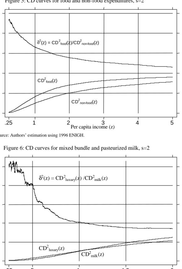
Empirical illustration

This section briefly applies the above normative and statistical tools to household-level data from Mexico’s 1996 ENIGH, a nationally representative survey with detailed income and consumption modules