Vadym Sakhno Mykola Sakhno
December 21, 2020
ABSTRACT
The Ising model was generalized to a system of cells interacting exclusively by presence of shared spins. Within the cells there are interactions of any complexity, the simplest intracell interactions come down to the Ising model. The system may be not only one-dimensional but also two-dimensional, three-dimensional, etc.
The purpose of the paper is to develop an approach to constructing the exact matrix model for any considered system in the simplest way. Without this, it is almost impossible to analyze complex systems. After trying a lot of ways, the approach has been simplified to suit first year students. Using the approach, the exact matrix model for a two-dimensional generalized Ising model was constructed.
The following approaches have already been developed to obtaining and analyzing partition function and various thermodynamic functions. They will be considered in following papers.
1
Introduction
1.1 Microreview
The Ising model arouses great interest in various fields. And even in comparatively narrow field of the Ising model exact solutions, there are thousands of publications. The authors have tried to develop their own approaches different from the published ones in order to get results worthy of Your attention. Therefore, the authors limited themselves to a microreview of only those works that are most directly related to their approaches. As foundation base of statistical mechanics, the authors use K. Huang [1], of Ising model exact solutions – L. Onsager [2], as fundamental review of exactly solved models – R.J. Baxter [3]. Among the numerous publications developing exact solutions, the closest seems to be P. Khrapov [4] and Yu.D. Panov [5]. And research directions were outlined by B.M. McCoy and J.-M. Maillard [6].
1.2 Systems and tasks under consideration
This paper considers systems depending on variables with a finite range of values (hereinafter, for brevity, each such variable is called spin, and the amount of its values - magnitude). These systems may have arbitrary: physical nature, the dimensions of space-time, geometry, other properties; but must have three given properties:
1. System energy E can be represented as the sum of energies of its parts called cells.
2. Each cell energy is the given function only of its own spins as well as internal and external parameters. Interaction between cells is performed exclusively through existence of shared spins. There are no other interactions between cells. The structure and parameters of different cells may vary.
3. There is such cell numbering that each cell has at least one spin belonging exclusively to cells with a lesser number.
For these systems, the following tasks are considered: 1. Construct the exact matrix model.
2. Using the exact matrix model, find the partition function exactly and analyse it Z=Xexp(− E
kB∗T
), (1)
where summing is performed over all possible values of all spins.
3. Using the partitioning function (1), find the thermodynamic functions exactly and analyze them: Helmholtz free energy A, magnetization M, magnetic susceptibilityχ, etc.
A=−kB∗T∗ln(Z), M =− ∂ ∂H( A kB∗T ), χ= ∂M ∂H. (2)
This paper considers only the first task, the rest ones will be discussed in following publications.
1.3 Notes
1. For d-magnitude spins, we assume that it has d values from(−d−1
2 )to(+
d−1
2 ), with step 1. For example,
2-magnitude spin has two values{−1
2,
1
2}, 3-magnitude spin has 3 values{−1, 0, 1}, etc.
2. The system may be split into cells by various ways. For example, some cells may be merged, and some other sell may be split. A shared part of two cells may be included in the first cell or the second cell or split in some way between these two cells. Such transformations do not influence the final result; however, they may simplify calculations.
3. The Ising model is obtained using the simplest energy function for cells. Thus, the considered systems are generalizations of the Ising model. For example, 4-spin cell considers not only interactions of its 4 spins with an external field and spin-spin interactions between nearest spins but also other spin-spin interactions as well as 3-spin and 4-spin interactions.
4. Typical cell numbering is suitable for typical systems.
1.4 Paper overview
Simple approach to construction of the exact matrix model for any considered system is developed in section 2. A simplified general example of this construction is shown in section 3.
A demonstration section was written initially. The exact matrix models were constructed for various one-dimensional systems there. But the authors got a comment on lack of novelty. Thus, the section was deleted.
The exact matrix model for a two-dimensional system is constructed in section 4.
2
A simple approach to construction of the exact matrix model for any considered system
The proposed approach consists of three simple steps: the first two steps are construction of two intermediate models and then a sought-for matrix model.
2.1 Construction of intermediate function model
Let the system consists ofN+ 2cells; each cell is assigned a unique numbern∈[0, N + 1]. The cell numbered 0 is called the start cell, the cell numberedN+ 1is called the finish cell, the remaining cells numberedn∈[1, N]are called internal cells.
A spin belonging to only one cell is called the local spin. The set of all local spins of the cell n is denoted byYn. Any
local spinynνof this set is numbered with a unique compound number consisted of two sub-numbers: n – cell number,ν
– serial number inside the cell. The set of all local spins of the system is denoted asY =Y0∪Y1∪Y2∪. . .∪YN∪YN+1.
Some local spins may have infinite range of values and even be continuous.
A spin belonging to two or more cells is called the shared spin. Any shared spinxnνis numbered with a unique compound
number consisted of two sub-numbers: n – the maximum number of the cell containing the spin,ν– serial number in shared spins having the first sub-number n. The set of all shared spins belonging to cell (not only having first sub-number n) is denoted byXn. The set of all shared spins of the system is denoted asX =X0∪X1∪X2∪. . .∪XN ∪XN+1.
Let us sum up in (1) over all local spins. Summation over continuous spin becomes integration. Of course, cells without local spins do not need to be summed over them. Thus, for each celln∈[0, N+ 1]we introduce cell functionZn(Xn)
Zn(Xn) = X Yn exp −En(Xn, Yn) kBT >0. (3)
Property 3 in subsection 1.2 implies that for each cell numberedn∈[1, N + 1]there is a non-empty subsetΥn ⊂Xn
of shared spins with the first sub-number n. Then summation over shared spins in (1) may be split into (N+1) partial summations Z = X ΥN+1 ZN+1(XN+1)∗ X ΥN ZN(XN)∗. . .∗ X Υn Zn(Xn)∗. . .∗ X Υ2 Z2(X2)∗ X Υ1 Z1(X1)∗Z0(X0), (4)
where each partial summationn∈[1, N+ 1]is performed over values of shared spins of setΥn.
The equation (4) uses the cell functions, so we call (4) the function model.
2.2 Construction of intermediate frame model
The function model (4) uses each cell function only in the values of its shared spins. Thus, each cell function generates a set of its values. Let us call the set a cell frame and enumerate its values as follows.
For eachdnν- magnitude shared spinxnν ∈[−dnν2−1, +dnν2−1]let us introduce a corresponding spin-numberinνlike
this
inν =xnν+
dnν−1
2 . (5)
The spin-numberinν ∈[0, dnν−1]is used for numbering values in any cell frame containing the spin.
The inverse equation for (5) is
xnν =inν−
dnν−1
2 . (6)
This results in a simple algorithm of constructing the frame for each cell functionZn(Xn). InZn(Xn)each spin
ofXnis substituted with its spin-number using (6). Let us denote the set of these spin-numbers asInand use it for
numbering in the cell frame. Then the cell frameZnInfor the cell functionZn(Xn)is
ZnIn=Zn(Xn(In))>0. (7)
Example. Let a cell functionZnhave three 2-magnitude spinsZn(xn+1, xn, xn−1). The cell frameZnin+1inin−1=
Zn in+1−12, in−12, in−1−12
consists of eight elements, for which spin-numbersin+1, in, in−1have two values
{0, 1}each. Namely: Zn000 =Zn −12,−12,−12,Zn001 =Zn −12,−12,12,Zn010 =Zn −12,12,−12,Zn011= Zn −12,12,12 ,Zn100=Zn 21,−12,−12 ,Zn101 =Zn 12,−12,12 ,Zn110=Zn 12,12,−12 ,Zn111=Zn 12,12,12 . Thus, set of spin-numbersin+1, in, in−1may be considered as a binary number having values from 0 to 7.
In the function model (4), substituting each spin with its spin-number, and each cell function with its frame constructs the frame model
Z= X I(ΥN+1) Z(N+1)IN+1∗ X I(ΥN) ZN IN ∗. . .∗ X I(Υn) ZnIn∗. . .∗ X I(Υ2) Z2I2∗ X I(Υ1) Z1I1∗Z0I0, (8)
whereI(Υn)withn∈[1, N+ 1]– spin-numbers set for spins of setΥn.
The constructing of the frame model may be substantiated more formally. In the function model (4), let us interpolate each cell function in the Lagrange form. Then the coefficients of Lagrange basis polynomials are the frame values. Taking into account the orthonormality of the Lagrange basis polynomials, we obtain the frame model (8).
2.3 Construction of the sought matrix model
When in the frame model (8) each cell frame is rewritten in the matrix form, then the summations turn into matrix multiplications. To do this, in the frame model (8) perform the following steps:
0. The frame of the start cellZ0I0is rewritten as a column vector
←− Z0.
1. Denote the result of the first summation as a column vector←A−1. Denote the frame of the first cellZ1I1 as a
matrix←Z→1 so that ←− A1= ←→ Z1∗ ←− Z0.
2. Denote the result of the second summation as a column vector←A−2. Denote the frame of the second cellZ2I2
as a matrix←Z→2so that ←− A2= ←→ Z2∗ ←− A1. ...
N. Denote the result of N-th summation as a column vector←−AN. Denote the frame of the N-th cellZN IN as a
matrix←Z→N so that ←− AN = ←→ ZN∗ ←−−− AN−1.
N+1. The frame of the finish cellZ(N+1)IN+1is rewritten as a row vector
−−−→
ZN+1. Then the resulting partitioning
function isZ=−−−→ZN+1∗
←− AN.
Combining all these steps, the sought-for matrix model is obtained
Z=−−−→ZN+1∗ ←→ ZN ∗. . .∗ ←→ Zn∗. . .∗ ←→ Z2∗ ←→ Z1∗ ←− Z0= −−−→ ZN+1∗ 1 Y n=N ←→ Zn ! ∗←Z−0. (9)
3
A general simplified example of obtaining the exact matrix model, and its analysis
In the function model (4) let us consider only the first summation from the start cell. The rest of the summations are considered similarly. Let cells 0 and 1 each have three 2-magnitude spins, and the first summation is
A1(x20, x30, x40) =
X
x10∈{−12,12}
Z1(x10, x20, x40)∗Z0(x10, x20, x30). (10)
3.1 Spin types with respect to summation
For spins of start cell functionZ0let us introduce the following types:
1. Spins belonging to the start and first cells exclusively and not belonging to any other cell. The summation “annihilates” them, so they are called “annihilated” spins. Property 3 in subsection 1.2 requires “annihilated”
spins to be present. There is one “annihilated” spinx10in (10).
2. Spins belonging to the start, first, and at least one more cell. The summation “processes” them and passes them further, so they are called “processed” spins. “Processed” spins may be missing. There is one “processed” spin x20in (10).
3. Spins not belonging to the first, but belonging to the start and at least one more cell. The summation just “passes” them further, so they are called “passed” spins. “Passed” spins may be missing. There is one “passed”
spinx30in (10).
The first cell has “destroyed” and “processed” spins shared with the start cell. In addition, the first cell may have spins of one more type:
4. Spins not belonging to the start, but belonging to the first and at least one more cell. The summation “creates” them, they are called “created” spins. There is one “created” spinx40in (10).
Thus, example (10) is general because it contains spins of all types. Simultaneously, this example is simplified because it contains only one spin of each type, and the spins are 2-magnitude.
3.2 Construction of the sought matrix model
First, from the function model (10) let us obtain the frame model in the form (8). In the function model, we need to substitute each spin with its spin-number, and each function with its frame. Frames of given cell functions Z0(x10, x20, x30)andZ1(x10, x20, x40)are calculated using (7). Moreover, this calculation is shown in detail in the
example after (7). The frame of the sought-for functionA1(x20, x30, x40)is just written. Then the frame model of (10)
is
A1i20i30i40 = X
i10∈{0,1}
Z1i10i20i40∗Z0i10i20i30. (11)
Let’s write (11) line by line. In the zero line:i20= 0, i30= 0, i40= 0; in the first line:i20= 0, i30= 0, i40= 1; . . . ;
in the seventh line:i20= 1, i30= 1, i40= 1
A1000=Z1000∗Z0000+Z1100∗Z0100, A1001=Z1001∗Z0000+Z1101∗Z0100, A1010=Z1000∗Z0001+Z1100∗Z0101, A1011=Z1001∗Z0001+Z1101∗Z0101, A1100=Z1010∗Z0010+Z1110∗Z0110, A1101=Z1011∗Z0010+Z1111∗Z0110, A1110=Z1010∗Z0011+Z1110∗Z0111, A1111=Z1011∗Z0011+Z1111∗Z0111. (12)
Let us introduce column vectorsA1andZ0and write (12) in matrix form
A1000 A1001 A1010 A1011 A1100 A1101 A1110 A1111 = Z1000 0 0 0 Z1100 0 0 0 Z1001 0 0 0 Z1101 0 0 0 0 Z1000 0 0 0 Z1100 0 0 0 Z1001 0 0 0 Z1101 0 0 0 0 Z1010 0 0 0 Z1110 0 0 0 Z1011 0 0 0 Z1111 0 0 0 0 Z1010 0 0 0 Z1110 0 0 0 Z1011 0 0 0 Z1111 ∗ Z0000 Z0001 Z0010 Z0011 Z0100 Z0101 Z0110 Z0111 , (13) or compactly ←− A1= ←→ Z1∗ ←− Z0. (14)
Hence the conclusions on the structure of the matrix←Z→1are
1. The matrix←Z→1 is non-negative.
2. The amount of columns in←Z→1is equal to the product of the magnitudes of “annihilated”, “processed” and
“passed” spins, that is, all spins of the start cell function (in this example it is 8).
3. The amount of non-zero columns in←Z→1 is equal to the product of the magnitudes of “annihilated” spins (in
this example it is 2).
4. The amount of rows in←Z→1is equal to the product of the magnitudes of “created”, “processed” and “passed”
spins (in this example it is 8).
5. The amount of non-zero rows in←Z→1 is equal to the product of the magnitudes of “created” spins (in this
example it is 2).
3.3 The simplest cyclic shift matrices
In (11) the start cell frameZ0i10i20i30 contains spin-numbersi20i30. The first sum frameA1i20i30i40contains the same
spin-numbers shifted to the left. Let us introduce cyclic left shift operatorPl, which for any vectorZi1i2i3performs the
Zi2i3i1 =Pl∗Zi1i2i3.
Let us move on to the matrix form
Z000 Z010 Z100 Z110 Z001 Z011 Z101 Z111 = 1 0 0 0 0 0 0 0 0 0 1 0 0 0 0 0 0 0 0 0 1 0 0 0 0 0 0 0 0 0 1 0 0 1 0 0 0 0 0 0 0 0 0 1 0 0 0 0 0 0 0 0 0 1 0 0 0 0 0 0 0 0 0 1 ∗ Z000 Z001 Z010 Z011 Z100 Z101 Z110 Z111 .
Hence the left cyclic shift matrix←P→l and its inverse as right cyclic shift matrix
←→ Pr = ←→ Pl−1 ←→ Pl = 1 0 0 0 0 0 0 0 0 0 1 0 0 0 0 0 0 0 0 0 1 0 0 0 0 0 0 0 0 0 1 0 0 1 0 0 0 0 0 0 0 0 0 1 0 0 0 0 0 0 0 0 0 1 0 0 0 0 0 0 0 0 0 1 , ←P→r = 1 0 0 0 0 0 0 0 0 0 0 0 1 0 0 0 0 1 0 0 0 0 0 0 0 0 0 0 0 1 0 0 0 0 1 0 0 0 0 0 0 0 0 0 0 0 1 0 0 0 0 1 0 0 0 0 0 0 0 0 0 0 0 1 . (15)
Then matrix←Z→1from (13) may be written in a form more convenient for analysis
←→ Zl = ←→ Zl∗ ←→ Pl ∗ ←→ Pr = Z1000 Z1100 0 0 0 0 0 0 Z1001 Z1101 0 0 0 0 0 0 0 0 Z1000 Z1100 0 0 0 0 0 0 Z1001 Z1101 0 0 0 0 0 0 0 0 Z1010 Z1110 0 0 0 0 0 0 Z1011 Z1111 0 0 0 0 0 0 0 0 Z1010 Z1110 0 0 0 0 0 0 Z1011 Z1111 ∗←P→r.
4
A two-dimensional system
In this paper, we restrict ourselves to considering only one of the two-dimensional systems, a particular case of which is easily diagonalized. The diagonalization will be considered in a following paper.
4.1 Description of the 2D system under consideration
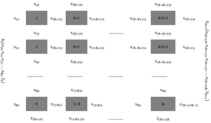
Let us consider the 2D model shown in Figure 1.
The system consists of(N+ 2)cells:N internal cells numbered from1toN, start cell numbered0, and finish cell numbered(N+ 1).
N internal cells formRrows. The lowest spin of a column continues into the highest spin of the next column (see x(R+1)0). Thus, cells are placed along a helix. The last column may be uncompleted.
Each internal cellnhas setXnof four shared 2-magnitude spins. The numbers of the upperxn0and the leftxn1spins
have their first sub-number equal to the cell numbern. Then the lower spin is numberedx(n+1)0as the upper one for
cell(n+ 1). And the right spin is numberedx(n+R)2as the left one for cell(n+R). Moreover, each internal celln
may contain an arbitrary set of local spinsYn. The internal cell energy is a given functionEn(Xn, Yn). Substituting it
into (3), we get the internal cell functionZn xn0, xn1, x(n+1)0, x(n+R)1
.
The start and finish cells each contain(R+ 1)shared spins and may contain arbitrary sets of local spins. Their energies are given functionsE0(x10, x11, x21, . . . , xR1, Y0)andEN+1 x(N+1)0, x(N+1)1, x(N+1)2, . . . , x(N+1)R, YN+1
Figure 1: The 2D system under consideration.
Substituting them into (3), we obtain the functions of the start and the finish cellsZ0(x10, x11, x21, . . . , xR1)and
ZN+1 x(N+1)0, x(N+1)1, x(N+1)2, . . . , x(N+1)R
.
4.2 Construction of the matrix model
Construction of the matrix model is similar to the general simplified example (section 3).
In the function model (4) let us consider only the first summation from the start cell. The rest of the summations are considered similarly. Let the result function of the first summation be denoted byA1. Then the first summation is
A1= X Υ1 Z1(X1)∗Z0(X0) = X Υ1 Z1 x10, x11, x20, x(1+R)1 ∗Z0(x10, x11, x21, . . . , xR1). (16)
SetX0of spins of the start cell functionZ0has spins of two types (see subsection 3.1): subset of two “annihilated”
spinsΥ1={x10, x11}and subset of(R−1)"passed" spins{x21, . . . , xR1}. SetX1of spins of the first cell function
Z1 also has spins of two types: the same subsetΥ1of two “annihilated” spins and subset of two “created” spins
x20, x(1+R)1 . Then the set of spins of the first result functionA1consisting of the "passed" and “created” spins is
x20, x21, . . . , xR1, x(1+R)1 .
Based on the conclusions from subsection 3.2, we can conclude the sought matrix←Z→1structure:
1. There are two 2-magnitude “annihilated” spins, so the amount of non-zero columns is22= 4.
2. There are(R+ 1)of 2-magnitude “annihilated” and “passed” spins, so the amount of columns is2R+1. 3. There are two 2-magnitude “created” spins, so the amount of non-zero rows is22= 4.
4. There are(R+ 1)of 2-magnitude “created” and “passed” spins, so the amount of rows is2R+1.
In (16), we need to substitute each spin with its spin-number and each function with its frame. Frames of given cell functionsZ0(x10, x11, x21, . . . , xR1)andZ1 x10, x11, x20, x(1+R)1
are calculated using (7). The frame of the first result functionA1 x20, x21, . . . , xR1, x(1+R)1
Let us describe in detail the frame of the first cell functionZ1 x10, x11, x20, x(1+R)1
. For each spinxnν ∈[−12, +12]
we introduce a corresponding spin-numberiν ∈[0,1]according to (6). Then, according to (7), the sought-for first cell
frame with 16 values is
Z1i10i11i20i(R+1)1 =Z1 i10− 1 2, i11− 1 2, i20− 1 2, i(R+1)1− 1 2 . (17)
After the described substitution of functions with frames and spins with spin-numbers in the function model (16), we obtain the frame model
A1i20i21...iR1i(1+R)1=
X
i10∈{0,1} i11∈{0,1}
Z1i10i11i20i(1+R)1∗Z0i10i11i21...iR1. (18)
Let us write (18) line by line
A100...00=Z10000∗Z0000...0+Z10100∗Z0010...0+Z11000∗Z0100...0+Z11100∗Z0110...0, A100...01=Z10001∗Z0000...0+Z10101∗Z0010...0+Z11001∗Z0100...0+Z11101∗Z0110...0, A100...10=Z10000∗Z0000...1+Z10100∗Z0010...1+Z11000∗Z0100...1+Z11100∗Z0110...1, A100...11=Z10001∗Z0000...1+Z10101∗Z0010...1+Z11001∗Z0100...1+Z11101∗Z0110...1, . . . A101...00=Z10000∗Z0001...0+Z10100∗Z0011...0+Z11000∗Z0101...0+Z11100∗Z0111...0, A101...01=Z10001∗Z0001...0+Z10101∗Z0011...0+Z11001∗Z0101...0+Z11101∗Z0111...0, A101...10=Z10000∗Z0001...1+Z10100∗Z0011...1+Z11000∗Z0101...1+Z11100∗Z0111...1, A101...11=Z10001∗Z0001...1+Z10101∗Z0011...1+Z11001∗Z0101...1+Z11101∗Z0111...1, . . . A110...00=Z10010∗Z0000...0+Z10110∗Z0010...0+Z11010∗Z0100...0+Z11110∗Z0110...0, A110...01=Z10011∗Z0000...0+Z10111∗Z0010...0+Z11011∗Z0100...0+Z11111∗Z0110...0, A110...10=Z10010∗Z0000...1+Z10110∗Z0010...1+Z11010∗Z0100...1+Z11110∗Z0110...1, A110...11=Z10011∗Z0000...1+Z10111∗Z0010...1+Z11011∗Z0100...1+Z11111∗Z0110...1, . . . A111...00=Z10010∗Z0001...0+Z10110∗Z0011...0+Z11010∗Z0101...0+Z11110∗Z0111...0, A111...01=Z10011∗Z0001...0+Z10111∗Z0011...0+Z11011∗Z0101...0+Z11111∗Z0111...0, A111...10=Z10010∗Z0001...1+Z10110∗Z0011...1+Z11010∗Z0101...1+Z11110∗Z0111...1, A111...11=Z10011∗Z0001...1+Z10111∗Z0011...1+Z11011∗Z0101...1+Z11111∗Z0111...1, . . . . (19)
Let us introduce column vectors←A−1and ←− Z0of dimension2R+1 ←− A1= A100...00 A100...01 A100...10 A100...11 . . . . . . A101...00 A101...01 A101...10 A101...11 . . . . . . A110...00 A110...01 A110...10 A110...11 . . . . . . A111...00 A111...01 A111...10 A111...11 . . . . . . , ←Z−0= Z0000...0 Z0000...1 . . . Z0001...0 Z0001...1 . . . Z0010...0 Z0010...1 . . . Z0011...0 Z0011...1 . . . Z0100...0 Z0100...1 . . . Z0101...0 Z0101...1 . . . Z0110...0 Z0110...1 . . . Z0111...0 Z0111...1 . . . . (20)
←→ ζ00= Z10000 0 . . . 0 0 . . . Z10100 0 . . . 0 0 . . . Z10001 0 . . . 0 0 . . . Z10101 0 . . . 0 0 . . . 0 Z10000 . . . 0 0 . . . 0 Z10100 . . . 0 0 . . . 0 Z10001 . . . 0 0 . . . 0 Z10101 . . . 0 0 . . . . . . . . . . . 0 0 . . . Z10000 0 . . . 0 0 . . . Z10100 0 . . . 0 0 . . . Z10001 0 . . . 0 0 . . . Z10101 0 . . . 0 0 . . . 0 Z10000 . . . 0 0 . . . 0 Z10100 . . . 0 0 . . . 0 Z10001 . . . 0 0 . . . 0 Z10101 . . . . . . . . . . . , ←→ ζ01= Z11000 0 . . . 0 0 . . . Z11100 0 . . . 0 0 . . . Z11001 0 . . . 0 0 . . . Z11101 0 . . . 0 0 . . . 0 Z11000 . . . 0 0 . . . 0 Z11100 . . . 0 0 . . . 0 Z11001 . . . 0 0 . . . 0 Z11101 . . . 0 0 . . . . . . . . . . . 0 0 . . . Z11000 0 . . . 0 0 . . . Z11100 0 . . . 0 0 . . . Z11001 0 . . . 0 0 . . . Z11101 0 . . . 0 0 . . . 0 Z11000 . . . 0 0 . . . 0 Z11100 . . . 0 0 . . . 0 Z11001 . . . 0 0 . . . 0 Z11101 . . . . . . . . . . . , ←→ ζ10= Z10010 0 . . . 0 0 . . . Z10110 0 . . . 0 0 . . . Z10011 0 . . . 0 0 . . . Z10111 0 . . . 0 0 . . . 0 Z10010 . . . 0 0 . . . 0 Z10110 . . . 0 0 . . . 0 Z10011 . . . 0 0 . . . 0 Z10111 . . . 0 0 . . . . . . . . . . . 0 0 . . . Z10010 0 . . . 0 0 . . . Z10110 0 . . . 0 0 . . . Z10011 0 . . . 0 0 . . . Z10111 0 . . . 0 0 . . . 0 Z10010 . . . 0 0 . . . 0 Z10110 . . . 0 0 . . . 0 Z10011 . . . 0 0 . . . 0 Z10111 . . . . . . . . . . . , ←→ ζ11= Z11010 0 . . . 0 0 . . . Z11110 0 . . . 0 0 . . . Z11011 0 . . . 0 0 . . . Z11111 0 . . . 0 0 . . . 0 Z11010 . . . 0 0 . . . 0 Z11110 . . . 0 0 . . . 0 Z11011 . . . 0 0 . . . 0 Z11111 . . . 0 0 . . . . . . . . . . . 0 0 . . . Z11010 0 . . . 0 0 . . . Z11110 0 . . . 0 0 . . . Z11011 0 . . . 0 0 . . . Z11111 0 . . . 0 0 . . . 0 Z11010 . . . 0 0 . . . 0 Z11110 . . . 0 0 . . . 0 Z11011 . . . 0 0 . . . 0 Z11111 . . . . . . . . . . . . (21) Then we get (14) ←− A1= ←→ Z1∗ ←− Z0,
←→ Z1= ←→ ζ00 ←→ ζ01 ←→ ζ10 ←→ ζ11 ! . (22)
And so on. In the end, we introduce the row vector for the finish cell−−−→ZN+1and get the matrix model (9)
Z=−−−→ZN+1∗ ←→ ZN ∗. . .∗ ←→ Zn∗. . .∗ ←→ Z2∗ ←→ Z1∗ ←− Z0= −−−→ ZN+1∗ 1 Y n=N ←→ Zn ! ∗←Z−0.
4.3 2D cyclic shift matrices
The structure of four2R×2Rmatrices←ζ→00,
←→ ζ01,
←→ ζ10,
←→
ζ11is similar to the structure of the matrix
←→
Z1from (13). As in
subsection 3.3, we introduce2R×2Rleft cyclic shift matrix←P→l and its inverse as right cyclic shift matrix
←→ Pr = ←→ Pl−1. ←→ Pl = 1 0 0 0 . . . 0 0 0 0 . . . . 0 0 1 0 . . . 0 0 0 0 . . . . . . . . 0 0 0 0 . . . 1 0 0 0 . . . . 0 0 0 0 . . . 0 0 1 0 . . . . . . . . 0 1 0 0 . . . 0 0 0 0 . . . . 0 0 0 1 . . . 0 0 0 0 . . . . . . . . 0 0 0 0 . . . 0 1 0 0 . . . . 0 0 0 0 . . . 0 0 0 1 . . . . . . . . , ←→ Pr = 1 0 . . . 0 0 . . . 0 0 . . . 0 0 . . . 0 0 . . . 0 0 . . . 1 0 . . . 0 0 . . . 0 1 . . . 0 0 . . . 0 0 . . . 0 0 . . . 0 0 . . . 0 0 . . . 0 1 . . . 0 0 . . . . . . . . . . . 0 0 . . . 1 0 . . . 0 0 . . . 0 0 . . . 0 0 . . . 0 0 . . . 0 0 . . . 1 0 . . . 0 0 . . . 0 1 . . . 0 0 . . . 0 0 . . . 0 0 . . . 0 0 . . . 0 0 . . . 0 1 . . . . . . . . . . . . (23)
Then the matrixZ1from (22) can be represented as
←→ Z1= ←→ B00 ←→ B01 ←→ B10 ←→ B11 ! ∗ ←→ Pr 0 0 ←P→r ! , (24)
where four2R×2Rblock matrices←→B00,
←→ B01,
←→ B10,
←→
B11are block-diagonal, along the diagonal of which there are
identical2×2blocks.
Consider elements of these four block matrices. An element with compound row numberi0i1i2. . . iR−1and compound
column numberj0j1j2. . . jR−1is non-zero only if all row sub-numbers except the last sub-numberR−1are equal to
the corresponding column sub-numbers. To emphasize this, we denote these four block matrices as2×2matrices with the number[R−1]. Then four block matrices from (24) are
←→ B00= ←→ ζ00∗ ←→ Pl = Z10000 Z10100 Z10001 Z10101 [R−1] = Z10000 Z10100 0 0 . . . 0 0 Z10001 Z10101 0 0 . . . 0 0 0 0 Z10000 Z10100 . . . 0 0 0 0 Z10001 Z10101 . . . 0 0 . . . . 0 0 0 0 . . . Z10000 Z10100 0 0 0 0 . . . Z10001 Z10101 , ←→ B01= ←→ ζ01∗ ←→ Pl = Z11000 Z11100 Z11001 Z11101 [R−1] = Z11000 Z11100 0 0 . . . 0 0 Z11001 Z11101 0 0 . . . 0 0 0 0 Z11000 Z11100 . . . 0 0 0 0 Z11001 Z11101 . . . 0 0 . . . . 0 0 0 0 . . . Z11000 Z11100 0 0 0 0 . . . Z11001 Z11101 , ←→ B10= ←→ ζ10∗ ←→ Pl = Z10010 Z10110 Z10011 Z10111 [R−1] = Z10010 Z10110 0 0 . . . 0 0 Z10011 Z10111 0 0 . . . 0 0 0 0 Z10010 Z10110 . . . 0 0 0 0 Z10011 Z10111 . . . 0 0 . . . . 0 0 0 0 . . . Z10010 Z10110 0 0 0 0 . . . Z10011 Z10111 , ←→ B11= ←→ ζ11∗ ←→ Pl = Z11010 Z11110 Z11011 Z11111 [R−1] = Z11010 Z11110 0 0 . . . 0 0 Z11011 Z11111 0 0 . . . 0 0 0 0 Z11010 Z11110 . . . 0 0 0 0 Z11011 Z11111 . . . 0 0 . . . . 0 0 0 0 . . . Z11010 Z11110 0 0 0 0 . . . Z11011 Z11111 . (25) Let us indicate the further used properties of2R×2Rshift matrices←P→
l and ←→ Pr ←→ PlR= ←→ PrR= ←→ 1 , (26)
where←→1 is2R×2Ridentity matrix.
Moreover, for arbitrary matrix←→B[r]the equalities hold
←→ Pr∗ ←→ B[r]∗ ←→ Pl = ←→ B[r+1], ←→ Pl ∗ ←→ B[r]∗ ←→ Pr = ←→ B[r−1]. (27)
5
Conclusion
1. In this paper, Section 2 describes the simple method for constructing the exact matrix model for the generalized Ising model.
2. Using this method, the exact matrix model is constructed for two-dimensional system (see Figure 1). It is (24) taking into account (23), (25) and (17).
References
[2] Lars Onsager. Crystal statistics. i. a two-dimensional model with an order-disorder transition.Physical Review, 65: 117–149, 1944.
[3] Rodney J. Baxterg.Exactly Solved Models in Statistical Mechanics. Elsevier Science, 2016.
[4] Pavel Khrapov. Disorder solutions for the partition functions of the two-dimensional ising-like models. 2020. URL
https://arxiv.org/abs/2011.10259.
[5] Yu.D. Panov. Local distributions of the 1d dilute ising model. 2020. URLhttps://arxiv.org/abs/2007. 04127.
[6] Barry M. McCoy and Jean-Marie Maillard. The importance of the ising model. Progress of Theoretical Physics, 127:791–817, 2012.