Modeling count time series following generalized linear models

(1)

Modeling Count Time Series

Following

Generalized Linear Models

Dissertation

Tobias Liboschik

In partial fulfillment of the

requirements for the degree of

Doktor der Naturwissenschaften

presented to the

Department of Statistics

TU Dortmund University

Advisors:

Prof. Dr. Roland Fried, TU Dortmund University

Prof. Dr. Konstantinos Fokianos, University of Cyprus

(2)

(3)

(4)

(5)

Abstract

Count time series are found in many different applications, e.g. from medicine, finance or industry, and have received increasing attention in the last two decades. The class of count time series following generalized linear models is very flexible and can describe serial correlation in a parsimonious way. The conditional mean of the observed process is linked to its past values, to past observations and to potential covariate effects. In this thesis we give a comprehensive formulation of this model class. We consider models with the identity and with the logarithmic link function. The conditional distribution can be Poisson or Negative Binomial. An important special case of this class is the so-called INGARCH model and its log-linear extension.

A key contribution of this thesis is theRpackage tscountwhich provides likelihood-based

estimation methods for analysis and modeling of count time series based on generalized linear models. The package includes methods for model fitting and assessment, prediction and intervention analysis. This thesis summarizes the theoretical background of these methods. It gives details on the implementation of the package and provides simulation results for models which have not been studied theoretically before. The usage of the package is illustrated by two data examples. Additionally, we provide a review of R

packages which can be used for count time series analysis. A detailed comparison of

tscount to those packages demonstrates that tscount is an important contribution which

extends and complements existing software.

A thematic focus of this thesis is the treatment of all kinds of unusual effects influencing the ordinary pattern of the data. This includes structural changes and different forms of outliers one is faced with in many time series. Our first study on this topic is concerned with retrospective detection of such changes. We analyze different approaches for modeling such intervention effects in count time series based on INGARCH models. Other authors treated a model where an intervention affects the non-observable underlying mean process at the time point of its occurrence and additionally the whole process thereafter via its dynamics. As an alternative, we consider a model where an intervention directly affects

(6)

the observation at its occurrence, but not the underlying mean, and then also enters the dynamics of the process. While the former definition describes an internal change of the system, the latter can be understood as an external effect on the observations due to e.g. immigration. For our alternative model we develop conditional likelihood estimation and, based on this, develop tests and detection procedures for intervention effects. Both models are compared analytically and using simulated and real data examples. The procedures for our new model work reliably and we find some robustness against misspecification of the intervention model.

The aforementioned methods are applied after the complete time series has been observed. In another study we investigate the prospective detection of structural changes, i.e. in real time. For example in public health, surveillance of infectious diseases aims at recognizing outbreaks of epidemics with only short time delays in order to take adequate action promptly. We point out that serial dependence is present in many infectious disease time series. Nevertheless it is still ignored by many procedures used for infectious disease surveillance. Using historical data, we design a prediction-based monitoring procedure for count time series following generalized linear models. We illustrate benefits but also pitfalls of using dependence models for monitoring.

Moreover, we briefly review the literature on model selection, robust estimation and robust prediction for count time series. We also make a first study on robust model identification using robust estimators of the (partial) autocorrelation.

Keywords: Count time series, generalized linear models, serial correlation, temporal

dependence, autoregressive models, regression models, likelihood, mixed Poisson, model selection, prediction, forecasting, statistical software, R, intervention analysis, level shifts, outliers, statistical process control, online monitoring, change point detection, aberration detection, outbreak detection, infectious disease surveillance, epidemiology, public health.

(7)

Chapter 1 Introduction

1.1 Motivation

Count time series appear naturally in various areas whenever a number of events per time period is observed over time. Examples for the wide range of applications in medicine are the weekly number of patients recruited for a clinical trial, the daily number of hospital admissions or the weekly number of epileptic seizures of a patient. An important example from epidemiology is the weekly number of registered infections by certain pathogens, which is routinely collected by public health authorities. Important objectives of such data analysis are the prediction of future values for adequate planning of resources, the detection of unusual values pointing at some epidemics or the proper description of e.g. seasonal patterns for better understanding and interpretation of data generating mechanisms. Examples from other fields are the number of stock market transactions per minute, from finance, or the hourly number of defect items, from industrial quality control.

Models for count time series should take into account that the observations are nonnegative integers and they should capture suitably the dependence among observations. A convenient and flexible approach is to employ the generalized linear model (GLM) methodology (Nelder and Wedderburn, 1972) for modeling the observations conditionally on the past information. This methodology is implemented by choosing a suitable distribution for count data and an appropriate link function. Such an approach is pursued by Fahrmeir and Tutz (2001, Chapter 6) and Kedem and Fokianos (2002, Chapters 1–4), among others. Another important class of models for time series of counts is based on the thinning operator, like the integer autoregressive moving average (INARMA) models, which, in a way, imitate the structure of the common autoregressive

(10)

moving average (ARMA) models (see the review article by Weiß, 2008). A different type of count time series models are the so-called state space models. We refer to the reviews of Fokianos (2011), Jung and Tremayne (2011), Fokianos (2012), Tjøstheim (2012) and Fokianos (2015) for an in-depth overview of models for count time series. Advantages of GLM-based models compared to the models which are based on the thinning operator are the following:

(a) They can describe covariate effects and negative correlations in a straightforward way.

(b) There is a rich toolkit available for this class of models.

State space models allow to describe even more flexible data generating processes than GLM models but at the cost of a more complicated model specification. On the other hand, GLM-based models yield predictions in a convenient manner due to their explicit formulation.

This thesis is concerned with methods for count time series based on generalized linear models. In the following section we give a comprehensive formulation of this model class.

1.2 Models

Denote a count time series by{Yt :t ∈N}. We will denote by{Xt :t ∈N}a time-varying

r-dimensional covariate vector, say Xt = (Xt,1, . . . , Xt,r)>. We model the conditional mean E(Yt|Ft−1) of the count time series by a process, say {λt : t ∈ N}, such that

E(Yt|Ft−1) = λt. Denote by Ft0 the history of the joint process {Yt, λt,Xt+1 : t ∈ N}

up to time t0 including the covariate information at time t0 + 1. The distributional assumption forYtgivenFt−1 is discussed later. We are interested in models of the general form g(λt) = β0+ p X k=1 βkeg(Yt−ik) + q X `=1 α`g(λt−j`) +η > Xt, (1.1) where g : _R+ _→

R is a link function and eg : N0 → R is a transformation function. The parameter vector η= (η1, . . . , ηr)> corresponds to the effects of covariates. In the terminology of GLMs we call νt = g(λt) the linear predictor. To allow for regression on arbitrary past observations of the response, define a set P = {i1, i2, . . . , ip} and integers 0 < i1 < i2. . . < ip < ∞, with p ∈ N0. This enables us to regress on the lagged observations Yt−i1, Yt−i2, . . . , Yt−ip. Analogously, define a set Q={j1, j2, . . . , jq}, q∈_N0 and integers 0< j1 < j2. . . < jq <∞, for regression on lagged conditional means

(11)

λt−j1, λt−j2, . . . , λt−jq. This case is covered by the theory for models with P ={1, . . . , p}

and Q = {1, . . . , q} by choosing p and q suitably and setting some model parameters

to zero. Our formulation is useful particularly when dealing with modeling stochastic seasonality (see Section 2.6.1, for an example). Specification of the model order, i.e., of the setsP andQ, are guided by considering the empirical autocorrelation functions of the

observed data. This approach is described for ARMA models in many time series analysis textbooks and transfers to the above model by employing its ARMA representation (see (A.4) in Appendix A.3). Parameter constraints which ensure stationarity and ergodicity

of two important special cases of (1.1) are given in Section 2.2.1.

We give several examples of model (1.1). Consider the situation where g and _eg equal

the identity, i.e., g(x) =_eg(x) =x. Furthermore, let P ={1, . . . , p}, Q={1, . . . , q} and η =0. Then model (1.1) becomes

λt=β0+ p X k=1 βkYt−k+ q X `=1 α`λt−`. (1.2)

Assuming further thatYtgiven the past is Poisson distributed, then we obtain an

integer-valued GARCH model of orderp andq, abbreviated as INGARCH(p,q). These models

are also known as autoregressive conditional Poisson (ACP) models. They have been

discussed by Heinen (2003), Ferland, Latour, and Oraichi (2006) and Fokianos, Rahbek, and Tjøstheim (2009), among others. An example of an INGARCH model with covariates is given in Section 2.5, where we fit a count time series model which includes intervention effects.

Consider again model (1.1) but now with the logarithmic link function g(x) = log(x),

e

g(x) = log(x+ 1) and P,Q as before. Then, we obtain a log-linear model of order pand q for the analysis of count time series. Indeed, setνt= log(λt)to obtain from (1.1) that

νt=β0+ p X k=1 βk log(Yt−k+ 1) + q X `=1 α`νt−`. (1.3)

This log-linear model is studied by Fokianos and Tjøstheim (2011), Woodard, Matteson, and Henderson (2011) and Douc, Doukhan, and Moulines (2013). We follow Fokianos and Tjøstheim (2011) in transforming past observations by employing the function e

g(x) = log(x+ 1), such that they are on the same scale as the linear predictor νt. These authors show that the addition of a constant c to each observation for avoiding zero

values does not affect inference; in addition they argue that a reasonable choice for cis 1.

Note that model (1.3) allows modeling of negative serial correlation, whereas model (1.2) accommodates positive serial correlation only. Additionally, (1.3) accommodates

(12)

covari-ates easier than (1.2) since the log-linear model implies positivity of the conditional mean process {λt}. The linear model (1.2) with covariates should be fitted with some care because it is limited to positive effects on {λt}. This is so because we need to ensure that the resulting mean process is positive. The effects of covariates on the response are multiplicative for model (1.3); they are additive though for model (1.2). For a discussion on the inclusion of time-dependent covariates see Fokianos and Tjøstheim (2011, Section 4.3).

In model (1.1) the effect of a covariate fully enters the dynamics of the process and propagates to future observations both by the regression on past observations and by the regression on past conditional means. The effect of such covariates can be seen as an internal influence on the data-generating process, which is why we refer to it as an

internal covariate effect. We also allow to include covariates in a way that their effect

only propagates to future observations by the regression on past observations but not directly by the regression on past conditional means. Following Liboschik, Kerschke, Fokianos, and Fried (2016), who make this distinction for the case of intervention effects described by deterministic covariates, we refer to the effect of such covariates as an

external covariate effect. Let e = (e1, . . . , er)> be a vector specified by the user with

ei = 1 if the i-th component of the covariate vector has an external effect and ei = 0 otherwise, i = 1, . . . , r. Denote by diag(e) a diagonal matrix with diagonal elements

given bye. The generalization of (1.1) allowing for both internal and external covariate

effects is given by g(λt) =β0+ p X k=1 βkeg(Yt−ik) + q X `=1 α` g(λt−j`)−η >_diag (e)Xt−j` +η>Xt. (1.4)

Basically, the effect of all covariates with an external effect is subtracted in the feedback terms such that their effect enters the dynamics of the process only via the observations. We refer to Chapter 3 (based on Liboschik et al., 2016) for an extensive discussion and

comparison of internal and external effects. It is our experience with these models that on the one hand an empirical discrimination between internal and external covariate effects is difficult but on the other hand there is some robustness against misspecification of the type of covariate effect.

So far we have only specified the mean of Yt|Ft−1 but not its distribution. Model (1.1) together with thePoisson assumption, i.e., Yt|Ft−1 ∼Poisson(λt), implies

P(Yt =y|Ft−1) =

λy_texp(−λt)

(13)

It holds VAR(Yt|Ft−1) = E(Yt|Ft−1) = λt. Hence in the case of a conditional Poisson response model the conditional mean is identical to the conditional variance of the observed process.

TheNegative Binomial distribution allows for a conditional variance to be larger than the

mean λt, which is often referred to as overdispersion and observed in many time series. Following Christou and Fokianos (2014), it is assumed that Yt|Ft−1 ∼ NegBin(λt, φ), where the Negative Binomial distribution is parametrized in terms of its mean with an additional dispersion parameter φ∈(0,∞) (Hilbe, 2011), i.e.,

P(Yt=y|Ft−1) = Γ(φ+y) Γ(y+ 1)Γ(φ) φ φ+λt φ λt φ+λt y , y∈_N0. (1.6)

In this case it again holds E(Yt|Ft−1) = λt but VAR(Yt|Ft−1) = λt+λ2t/φ, i.e., the conditional variance increases quadratically with λt. The Poisson distribution is a limiting case of the Negative Binomial when φ → ∞.

Note that the Negative Binomial distribution belongs to the class of mixed Poisson processes. A mixed Poisson process is specified by setting Yt=Nt(0, Ztλt], where {Nt} are i.i.d. Poisson processes with unit intensity and {Zt}are i.i.d. random variables with mean 1 and variance σ2, independent of {Yt}. When {Zt} is an i.i.d. process of Gamma random variables, then we obtain the Negative Binomial process with σ2 = 1/φ. We

refer to σ2 as the overdispersion coefficient because it is proportional to the extent of

overdispersion of the conditional distribution. The limiting case of σ2 _{= 0}_corresponds to the Poisson distribution, i.e., no overdispersion. The estimation procedure we study is not confined to the Negative Binomial case but to any mixed Poisson distribution. However, the Negative Binomial assumption is required for prediction intervals and model assessment; these topics are discussed in Sections 2.3 and 2.4.

1.3 Outline

Chapter 2 introduces the R packagetscount which implements methods for the class of

count time series following GLMs. This package includes methods for model fitting and assessment, prediction and intervention analysis. The chapter summarizes the theoretical background of these methods. It gives details on the implementation of the package and provides simulation results for models which have not been studied theoretically before. The usage of the package is illustrated by two data examples. Additionally, we provide a review of R packages which can be used for count time series analysis. This includes a

(14)

detailed comparison of tscount to those packages. The chapter is based on a manuscript

entitled “tscount: AnRpackage for Analysis of Count Time Series Following Generalized

Linear Models” which is currently under revision for Journal of Statistical Software. A

previous version of that manuscript has been published as a discussion paper (Liboschik, Fokianos, and Fried, 2015) and the most recent version is available as a vignette of the package.

In many applications, unusual external effects or measurement errors can lead to either sudden or gradual changes in the structure of the data, so-called intervention effects. A goal of an intervention analysis is to examine the effect of known interventions, for example to judge whether a policy change had the intended impact, or to search for unknown intervention effects and to find explanations for them. Chapter 3 studies different approaches for modeling intervention effects by deterministic covariates, focusing on INGARCH models from the class of GLM-based count time series models. Fokianos and Fried (2010) treated a model where an intervention has an internal effect according to the definition in the previous section, which describes an internal change of the system. We consider an alternative model where an intervention has an external effect on the observations due to e.g. immigration. For our alternative model we develop conditional likelihood estimation and, based on this, tests and detection procedures for intervention effects. We compare both models analytically and using simulated and real data examples. Our simulations confirm that the procedures for our new model perform well. It turns out that there is some robustness against misspecification of the intervention model. The chapter is based on the article “Modelling interventions in INGARCH processes” published in the International Journal of Computer Mathematics (Liboschik et al., 2016,

accepted for publication in July 2014).

The aforementioned methods are applied after the complete time series has been observed. Chapter 4 investigates the prospective detection of structural changes, i.e. in real time. For example in public health, surveillance of infectious diseases aims at recognizing outbreaks of epidemics with only short time delays in order to take adequate action promptly. We point out that serial dependence is present in many infectious disease time series. Nevertheless it is still ignored by many procedures used for infectious disease surveillance. This chapter studies how accommodating temporal dependence can improve monitoring procedures. Using historical data, we design a prediction-based monitoring procedure for count time series following GLMS. Our simulations and a data example demonstrate that such a procedure can substantially improve the immediate detection of outbreaks but that its dependence on previous observations may also yield undesired effects in some situations. We discuss some ideas how to utilize the promising features of dependent models for monitoring and at the same time to overcome their weakness.

(15)

Chapter 5 discusses three further topics, all of particular interest in the context of infectious disease surveillance, and points to directions where further research is needed. Section 5.1 reviews some further tools for model selection. The other two sections are concerned with robust methods which work reliably in the presence of outliers or intervention effects. Section 5.2 is a first study on robust identification of the model order for count time series with the robustly estimated (partial) autocorrelation function. This Section is based on Section 4 of the article “On Outliers and Interventions in Count Time Series following GLMs” published in the Austrian Journal of Statistics (Fried, Liboschik,

Elsaied, Kitromilidou, and Fokianos, 2014, Sections 4 and 5 are written by the author of this thesis). Section 5.3 reviews robust methods for parameter estimation and prediction. Chapter 6 concludes this thesis with a brief summary of its most important results.

(16)

(17)

Chapter 2 Basic methods and implementation

2.1 Introduction

Recently, there has been an increasing interest in regression models for time series of counts and a considerable number of publications on this subject has appeared in the literature. However, many of the proposed methods are not yet available in a statistical software package and hence they cannot be applied easily. We aim at filling this gap and publish a package named tscount for the popular free and open source software

environment R (R Core Team, 2016). In fact, our main goal is to develop software

for models whose conditional mean depends on previous observations and on its own previous values. These models are quite analogous to the generalized autoregressive conditional heteroscedasticity (GARCH) models (Bollerslev, 1986) which were proposed for describing the conditional variance.

In the first version of the package tscount we provide likelihood-based methods for the

framework of count time series following GLMs. Some simple autoregressive models can be fitted with standard software by treating the observations as if they were independent (see Section 2.7 and Appendix A.3), for example, using theRfunctionglm. However, these

procedures are in general not tailored for dependent data and may yield invalid model fits. The implementation in the packagetscountallows for a more general dependence structure

which is specified conveniently by the user. We consider general time series models whose conditional mean may depend on time-varying covariates, previous observations and, similar to the conditional variance of a GARCH model, on its own previous values. The usage and output of our functions is in parts inspired by the R functions arima andglm

in order to provide a familiar user experience. Furthermore tscountis object-oriented and

(18)

other Rfunctions available which can be employed for analyzing count time series. Many

of those are related to GLMs and have been developed for independent observations but are, with some limitations, also capable to describe simple forms of serial dependence. There are also some functions available for extending such models to time series. Another group of functions handles state space models for count time series. We briefly review these functions and the corresponding model classes in Section 2.7 and compare them to tscount. As it turns out, there are special cases for which our model corresponds to

existing ones. In these cases we obtain quite similar results with functions from some other packages, thus confirming the reliability of our package. However, many features of

tscount, like the flexible dependence structure, outreach the capability of other packages.

Admittedly, some packages provide features like zero-inflation or more general forms of the linear predictor which cannot be accommodated yet by tscount but could possibly

be included in future versions. As a conclusion, this package is a valuable addition to the

R environment which fills some significant gaps associated with time series fitting.

The functionality of tscount partly goes beyond the theory available in the literature

since theoretical investigation of these models is still an ongoing research theme. For instance the problem of accommodating covariates in such GLM-type count time series models or fitting a mixed Poisson log-linear model have not been studied theoretically. We have checked their appropriateness by simulations reported in Appendix B. However, some care should be taken when applying the package’s programs to situations which are not covered by existing theory.

This chapter is organized as follows. At first the theoretical background of the methods included in the package is briefly summarized with references to the literature for more details. Section 2.2 describes quasi maximum likelihood estimation of the unknown model parameters and gives some details regarding its implementation. Section 2.3 treats prediction with such models. Section 2.4 sums up tools for model assessment. Section 2.5 discusses procedures for the detection of interventions. Section 2.6 demonstrates the usage of the package with two data examples. Section 2.7 reviews other R packages

which are capable to model count time series and compares them with our package. Finally, Section 2.8 gives an outlook on possible future extensions of our package. In the Appendix we give further details and we confirm empirically some of the new methods that we discuss but which have not been studied, as of yet.

(19)

2.2 Estimation and inference

2.2.1 Estimation

Thetscountpackage fits models of the form (1.1) by quasi conditional maximum likelihood

(ML) estimation (function tsglm). If the Poisson assumption holds true, then we obtain

an ordinary ML estimator. However, under the mixed Poisson assumption we obtain a quasi-ML estimator. Denote by θ = (β0, β1, . . . , βp, α1, . . . , αq, η1, . . . , ηr)> the vector of regression parameters. Regardless of the distributional assumption, the parameter space for the INGARCH model (1.2) with covariates is given by

Θ = ( θ ∈_Rp+q+r+1 _: _β 0 >0, β1, . . . , βp, α1, . . . , αq, η1, . . . , ηr ≥0, p X k=1 βk+ q X `=1 α`<1 ) .

The intercept β0 must be positive and all other parameters must be nonnegative to ensure positivity of the conditional mean λt. The other condition ensures that the fitted model has a stationary and ergodic solution with moments of any order (Ferland et al.,

2006; Fokianoset al., 2009; Doukhan, Fokianos, and Tjøstheim, 2012); see also Tjøstheim

(2015) for a recent review. For the log-linear model (1.3) with covariates the parameter space is taken to be Θ = ( θ ∈_Rp+q+r+1 _: _|_β 1|, . . . ,|βp|,|α1|, . . . ,|αq|<1, p X k=1 βk+ q X `=1 α` <1 ) ,

see Appendix A.1 for a discussion. Christou and Fokianos (2014) point out that with the parametrization (1.6) of the Negative Binomial distribution the estimation of the regression parameters θ does not depend on the additional dispersion parameterφ. This

allows to employ a quasi maximum likelihood approach based on the Poisson likelihood to estimate the regression parameters θ, which is described below. The nuisance parameter

φ is then estimated separately in a second step. This approach is different from a full

maximum likelihood estimation based on the Negative Binomial distribution, which for example has been implemented in the function glm.nbin the Rpackage MASS(Venables

and Ripley, 2002). In that algorithm, maximization of the Negative Binomial likelihood for an estimated dispersion parameterφand estimation ofφgiven the estimated regression

parameters θ are iterated until convergence. The quasi negative binomial approach has

been chosen for simplicity and its usefulness on deriving consistent estimators when the model for λt has been correctly specified (see also Ahmad and Francq, 2016).

(20)

The log-likelihood, score vector and information matrix are derived conditionally on pre-sample values of the time series and the conditional mean process {λt}, precisely on

F0. An appropriate initialization is needed for their evaluation, which is discussed in the next subsection. For a vector of observations y = (y1, . . . , yn)>, the conditional quasi log-likelihood function, up to a constant, is given by

`(θ) = n X t=1 logpt(yt;θ) = n X t=1 ytln(λt(θ))−λt(θ) , (2.1)

where pt(y;θ) =P(Yt =y|Ft−1)is the probability density function of a Poisson distribu-tion as defined in (1.5). The condidistribu-tional mean is regarded as a funcdistribu-tionλt: Θ→R+ and thus it is denoted by λt(θ)for all t. The conditional score function is the (p+q+r+ 1) -dimensional vector given by

Sn(θ) = ∂`(θ) ∂θ = n X t=1 yt λt(θ) −1 ∂λt(θ) ∂θ . (2.2)

The vector of partial derivatives∂λt(θ)/∂θ can be computed recursively by the recursions given in Appendix A.2. Finally, the conditional information matrix is given by

Gn(θ;σ2) = n X t=1 COV ∂`(θ;Yt) ∂θ Ft−1 = n X t=1 1 λt(θ) + σ2 ∂λt(θ) ∂θ ∂λt(θ) ∂θ > . (2.3)

In the case of the Poisson assumption it holds σ2 _{= 0} and in the case of the Negative Binomial assumptionσ2 _{= 1}_/φ. For the ease of notation let _G∗

n(θ) = Gn(θ; 0), which is the conditional information matrix in case of a Poisson distribution.

The quasi maximum likelihood estimator (QMLE) θb_n of θ, assuming that it exists, is the solution of the non-linear constrained optimization problem

b

θ :=bθ_n= arg max θ∈Θ

`(θ). (2.4)

Denote the fitted values by bλ_t = λ_t(θb). Following Christou and Fokianos (2014), the dispersion parameterφ of the Negative Binomial distribution is estimated by solving the

equation n X t=1 (Yt−bλ_t)2 b λt+bλ2_t/φb) =n−(p+q+r+ 1), (2.5)

(21)

which is based on Pearson’s χ2 statistic. The variance parameter σ2 is estimated by

b

σ2 _{= 1}_/

b

φ. For the Poisson distribution we set σ_b2 _{= 0}_{. Strictly speaking, the log-linear} model (1.3) does not fall into the class of models considered by Christou and Fokianos (2014). However, results obtained by Douc et al. (2013) (for p=q= 1) and Sim (2016)

(for p = q) allow us to use this estimator also for the log-linear model. This issue is

addressed by simulations in Appendix B.2, which support that the estimator obtained by (2.5) provides good results also for models with the logarithmic link function.

2.2.2 Inference

Inference for the regression parameters is based on the asymptotic normality of the QMLE, which has been studied by Fokianos et al. (2009) and Christou and Fokianos

(2014) for models without covariates. For a well behaved covariate process {Xt} we conjecture that √ n b θn−θ0 _d −→Np+q+r+1 0, G−_n1(bθn;bσ 2 )G∗_n(bθn)Gn−1(θbn;σb 2 ) , (2.6)

as n→ ∞, where θ0 denotes the true parameter value andσb

2 _{is a consistent estimator} of σ2. We suppose that this applies under the same assumptions usually made for the

ordinary linear regression model (see for example Demidenko, 2013, p. 140 ff.). For deterministic covariates these assumptions are ||Xt||< c, where|| · || denotes the usual Euclidean norm, i.e., the covariate process is bounded, andlimn→∞n−1P_t=1n XtX>t =A, wherecis a constant andAis a nonsingular matrix. For stochastic covariates it is assumed

that the expectations E(Xt) and E XtX>t

exist and that E XtX>t

is nonsingular. The assumptions imply that the information on each covariate grows linearly with the sample size and that the covariates are not linearly dependent. Fuller (1996, Theorem 9.1.1) shows asymptotic normality of the least squares estimator for a regression model with time series errors under even more general conditions which allow the presence of certain types of trends in the covariates. For the special case of a Poisson model with the identity link, Agosto, Cavaliere, Kristensen, and Rahbek (2015) show asymptotic normality of the MLE for a model with covariates that are functions of Markov processes with finite second moments and that are not collinearly related to the response. The asymptotic normality of the QMLE in our context is supported by the simulations presented in Appendix B.1. A formal proof requires further research. To avoid numerical instabilities when inverting Gn(bθ_n;

b

σ2) we apply an algorithm which makes use of the

(22)

As an alternative method to the normal approximation (2.6) for obtaining standard errors and confidence intervals (functionse) we include a parametric bootstrap procedure

(argument B), for which computation time is many times higher. Accordingly, B time

series are simulated from the model fitted to the original data. The empirical standard errors of the parameter estimates for these B time series are the bootstrap standard

errors. Confidence intervals are based on quantiles of the bootstrap sample, see Efron and Tibshirani (1993, Chapter 13). This procedure can compute standard errors and confidence intervals both forθb and _bσ2. In our experienceB = 500yields stable results.

2.2.3 Implementation

This section and Appendix A provide some details on the implementation of the function

tsglm and explain its technical arguments. The default settings of this arguments are

chosen wisely based on plenty of experiments and should be sufficient for most situations though.

The parameter restrictions which are imposed by the conditionθ∈Θcan be formulated as

dlinear inequalities. This means that there exists a matrixU of dimensiond×(p+q+r+1)

and a vector c of length d, such thatΘ ={θ | U θ ≥c}. For the linear model (1.2) one

needs d=p+q+r+ 2 constraints to ensure nonnegativity of the conditional meanλt and stationarity of the resulting process. For the log-linear model (1.3) there are not any constraints on the intercept term and on the covariate coefficients; henced = 2(p+q+ 1).

In order to enforce strict inequalities the respective constraints are tightened by an arbitrarily small constant ξ >0; this constant is set to ξ = 10−6 by default (argument

slackvar).

For solving numerically the maximization problem (2.4) we employ by default the function

constrOptim. This function applies an algorithm described by Lange (1999, Chapter

14), which essentially enforces the constraints by adding a barrier value to the objective function and then employs an algorithm for unconstrained optimization of this new objective function, iterating these two steps if necessary. By default the quasi-Newton Broyden-Fletcher-Goldfarb-Shanno (BFGS) algorithm is employed for the latter task of unconstrained optimization, which additionally makes use of the score vector (2.2). It is possible to tune the optimization algorithm and even to employ an unconstrained optimization (argument final.control).

Note that the log-likelihood (2.1) and the score (2.2) are given conditional on unobserved pre-sample values. They depend on the linear predictor and its partial derivatives, which

(23)

can be computed recursively using any initialization. We give the recursions and present several strategies for their initialization in Appendix A.2 (arguments init.method and

init.drop). Christou and Fokianos (2014, Remark 3.1) show that the effect of the

initialization vanishes asymptotically. Nevertheless, from a practical point of view the initialization of the recursions is crucial. Especially in the presence of strong serial dependence, the resulting estimates can differ substantially even for long time series with 1000 observations; see the simulated example in Table A.1 in Appendix A.2.

Solving the non-linear optimization problem (2.4) requires a starting value for the parameter vector θ. This starting value can be obtained from fitting a simpler model for

which an estimation procedure is readily available. We consider either to fit a GLM or to fit an ARMA model. A third possibility is to fit a naive i.i.d. model without covariates. Furthermore, the user can assign fixed values. All these possibilities are available by the argument start.control. It turns out that the optimization algorithm converges very

reliably even if the starting values are not close to the global optimum of the likelihood. A starting value which is closer to the global optimum usually requires fewer iterations until convergence. However, we have encountered some examples where starting values close to a local optimum, obtained by one of the first two aforementioned methods, do not yield the global optimum. Consequently, we recommend fitting the naive i.i.d. model without covariates to obtain starting values. More details on these approaches are given in Appendix A.3.

2.3 Prediction

In terms of the mean square error, the optimal 1-step-ahead predictor Yb_n+1 for Y_n+1, given Fn, i.e., the past of the process up to time n and potential covariates at time n+ 1, is the conditional expectation λn+1 given in (1.1) (S3 method of function predict). By construction of the model the conditional distribution of Yb_n+1 is a Poisson (1.5) respec-tively Negative Binomial (1.6) distribution with mean λn+1. An h-step-ahead prediction

b

Yn+h forYn+h is obtained by recursive 1-step-ahead predictions, where unobserved values

Yn+1, . . . , Yn+h−1 are replaced by their respective 1-step-ahead prediction,h ∈ N. The

distribution of this h-step-ahead predictionYbn+h is not known analytically but can be approximated numerically by a parametric bootstrap procedure, which is described below. In applications, λn+1 is substituted by its estimator bλ_n+1 =λ_n+1(θb), which depends on the estimated regression parameters bθ. The dispersion parameter φ of the Negative Binomial distribution is replaced by its estimator φb. Note that plugging in the estimated

(24)

parameters induces additional uncertainty to the predictive distribution. This estimation uncertainty is not taken into account for the construction of prediction intervals described in the following paragraphs.

Prediction intervals for Yn+h with a given coverage rate 1−α (argument level) are designed to cover the true observation Yn+h with a probability of1−α. Simultaneous prediction intervals achieving a global coverage rate for Yn+1, . . . , Yn+h can be obtained by a Bonferroni adjustment of the individual coverage rates to 1−α/h each (argument

global = TRUE).

There are two different principles for constructing predictions intervals available which in practice often yield identical intervals. Firstly, the limits can be the(α/2)- and(1−α/2)

-quantile of the (approximated) predictive distribution (argumenttype = "quantiles").

Secondly, the limits can be chosen such that the interval has minimal length given that, according to the (approximated) predictive distribution, the probability that a value falls into this interval is at least as large as the desired coverage rate1−α (argumenttype =

"shortest").

One-step-ahead prediction intervals can be straightforwardly obtained from the condi-tional distribution (argument method = "conddistr"). Prediction intervals obtained

by a parametric bootstrap procedure (argument method = "bootstrap") are based on

B simulations of realizations y_n+1(b) , . . . , y_n+h(b) from the fitted model, b = 1, . . . , B

(argu-ment B). To obtain an approximative prediction interval for Yn+h one can either use the empirical (α/2)- and(1−α/2)-quantile of y_n+h(1) , . . . , y(B)_n+h (if type = "quantiles") or

find the shortest interval which contains at least d(1−α)·Beof these observations (if

type = "shortest"). This bootstrap procedure can be accelerated by distributing it

to multiple cores simultaneously (argument parallel = TRUE), which requires a

com-puting cluster registered by the R package parallel (see the help page of the function

setDefaultCluster).

2.4 Model assessment

Tools originally developed for generalized linear models as well as for time series can be utilized to asses the model fit and its predictive performance. Within the class of count time series following generalized linear models it is desirable to asses the specification of the linear predictor as well as the choice of the link function and of the conditional distribution. The tools presented in this section facilitate the selection of an adequate model for a given data set. Note that all tools are introduced as in-sample versions,

(25)

meaning that the observations y1. . . , yn are used for fitting the model as well as for assessing the obtained fit. However, it is straightforward to apply such tools as out-of-sample criteria.

Recall that the fitted values are denoted by λbt=λt(θb). Note that these do not depend on the chosen distribution, because the mean is the same regardless of the response distribution. There are various types of residuals available (S3 method of function

residuals). Response (or raw) residuals (argument type = "response") are given by

rt =yt−bλ_t, (2.7)

whereas a standardized alternative are Pearson residuals (argument type = "pearson")

r_tP = (yt−bλ_t)/ q b λt+bλ2_t b σ2_, (2.8)

or the more symmetrically distributed standardized Anscombe residuals (argument type

= "anscombe") rA_t = 3/bσ 2 _{1 +}_y tbσ 22/3 − 1 +bλ_t b σ22/3 + 3 y_t2/3−λb 2/3 t 2 bλ_t+λb2_t_bσ2 1/6 , (2.9)

for t= 1, . . . , n(see for example Hilbe, 2011, Section 5.1). The empirical autocorrelation

function of these residuals is useful for diagnosing serial dependence which has not been explained by the fitted model. A plot of the residuals against time can reveal changes of the data generating process over time. Furthermore, a plot of squared residuals r_t2

against the corresponding fitted values bλ_t exhibits the relation of mean and variance and might point to the Poisson distribution if the points scatter around the identity function or to the Negative Binomial distribution if there exists a quadratic relation (see Ver Hoef and Boveng, 2007).

Christou and Fokianos (2015b) and Jung and Tremayne (2011) extend tools for assessing the predictive performance to count time series, which were originally proposed by Gneiting, Balabdaoui, and Raftery (2007) and others for continuous data and trans-ferred to independent but not identically distributed count data by Czado, Gneiting, and Held (2009). These tools follow the prequential principle formulated by Dawid

(1984), depending only on the realized observations and their respective forecast dis-tributions. Denote by Pt(y) = P Yt ≤ y|Ft−1

the cumulative distribution function (c.d.f.), by pt(y) = P Yt = y|Ft−1

the probability density function, y ∈ _N0, and by

υt=

p

(26)

a Poisson distribution with mean bλt or a Negative Binomial distribution with mean bλt and overdispersion coefficient σb

2 _{(recall Section 2.3 on 1-step-ahead prediction).}

A tool for assessing the probabilistic calibration of the predictive distribution (see Gneiting et al., 2007) is the probability integral transform (PIT), which will follow a

uniform distribution if the predictive distribution is correct. For count data Czado et al.

(2009) define a non-randomized PIT value for the observed value yt and the predictive distribution Pt(y) by Ft(u|y) =            0, u≤Pt(y−1) u−Pt(y−1) Pt(y)−Pt(y−1) , Pt(y−1)< u < Pt(y) 1, u≥Pt(y) .

The mean PIT is then given by

F(u) = 1 n n X t=1 Ft(u|yt), 0≤u≤1.

To check whetherF(u)is the c.d.f. of a uniform distribution Czado et al.(2009) propose

plotting a histogram withHbins, where binhhas the heightfj =F(h/H)−F((h−1)/H),

h = 1, . . . , H (function pit). By default H is chosen to be 10. A U-shape indicates

underdispersion of the predictive distribution, whereas an upside down U-shape indicates overdispersion. Gneitinget al. (2007) point out that the empirical coverage of central,

e.g., 90% prediction intervals can be read off the PIT histogram as the area under the 90% central bins.

Marginal calibration is defined as the difference of the average predictive c.d.f. and the

empirical c.d.f. of the observations, i.e.,

1 n n X t=1 Pt(y)− 1 n n X t=1 1(yt≤y) (2.10)

for all y ∈ _R. In practice we plot the marginal calibration for values y in the range

of the original observations (Christou and Fokianos, 2015b) (function marcal). If the

predictions from a model are appropriate the marginal distribution of the predictions resembles the marginal distribution of the observations and (2.10) should be close to zero. Major deviations from zero point to model deficiencies.

Gneitinget al.(2007) show that the calibration assessed by a PIT histogram or a marginal

(27)

Scoring rule Abbreviation Definition

squared error score sqerror (yt−λt)2 normalized squared error score normsq (yt−λt)2/υt2 Dawid-Sebastiani score dawseb (yt−λt)2/υt2+ 2 log(υt) logarithmic score logarithmic −log(pt(yt)) quadratic (or Brier) score quadratic −2pt(yt) +kptk

2 spherical score spherical −pt(yt)/kptk ranked probability score rankprob P∞_y=0(Pt(y)−1(yt≤y))2 Table 2.1: Definitions of proper scoring rules s(Pt, yt) (cf. Czado et al., 2009) and their abbreviations in the package; kptk

2

=P∞_y=0p2 t(y).

They advocate to favor the model with the maximal sharpness among all sufficiently calibrated models. Sharpness is the concentration of the predictive distribution and can be measured by the width of prediction intervals. A simultaneous assessment of calibration and sharpness summarized in a single numerical score can be accomplished by

proper scoring rules (Gneitinget al., 2007). Denote a score for the predictive distribution

Pt and the observationyt by s(Pt, yt). A number of possible proper scoring rules is given in Table 2.1. The mean score for each corresponding model is given by Pn

t=1s(Pt, yt)/n. Each of the different proper scoring rules captures different characteristics of the predictive distribution and its distance to the observed data (function scoring). Except for the

normalized error score, the model with the lowest score is preferable. The mean squared error score is the only one which does not depend on the distribution and is also known as mean squared prediction error. The mean normalized squared error score measures the variance of the Pearson residuals and is close to one if the model is adequate. The Dawid-Sebastini score is a variant of this with an extra term to penalize overerstimation of the standard deviation.

Other popular tools are model selection criteria like Akaike’s information criterion (AIC) and the Bayesian information criterion (BIC) (functions AIC and BIC). The model with

the lowest value of the respective information criterion is preferable. Denote the log-likelihood by `e(θb,

b

σ2) =Pn

t=1log (pt(yt)). Note that this is the true and not the quasi log-likelihood given in (2.1). Furthermore, e`(bθ,_bσ2) includes all constant terms which have been omitted on the right hand side of (2.1). The AIC and BIC are given by AIC=−2e`(bθ, b σ2_{) + 2}_df _{and BIC}₌₋₂ e `(bθ, b σ2_{) + log(}_n

eff)df, respectively. Here df is the total number of parameters (including the dispersion coefficient) and neff the number of effective observations (excluding those only used for initialization when argument

init.drop = TRUE). The BIC generally yields more parsimonious models than the AIC.

(28)

(2.1) but not`e(θ, σ2). In such cases the quasi information criterion (QIC), proposed by Pan (2001) for regression analysis based on the generalized estimating equations, is a properly adjusted alternative to the AIC (functionQIC). We have verified by a simulation

reported in Appendix B.3 that in case of a Poisson distribution the QIC approximates the AIC quite satisfactory.

2.5 Intervention analysis

In many applications sudden changes or extraordinary events occur. Box and Tiao (1975) refer to such special events as interventions. This could be for example the outbreak of an epidemic in a time series which counts the weekly number of patients infected with a particular disease. It is of interest to examine the effect of known interventions, for example to judge whether a policy change had the intended impact, or to search for unknown intervention effects and find explanations for them a posteriori.

Fokianos and Fried (2010, 2012) model interventions affecting the location by including a deterministic covariate of the formδt−τ₁₍_t_≥_τ₎_{, where}_τ _{is the time of occurrence and} the decay rateδ is a known constant (functioninterv_covariate). This covers various

types of interventions for different choices of the constant δ: a singular effect for δ= 0

(spiky outlier), an exponentially decaying change in location for δ ∈ (0,1) (transient

shift) and a permanent change of location for δ = 1(level shift). Similar to the case of

covariates, the effect of an intervention is essentially additive for the linear model and multiplicative for the log-linear model. However, the intervention enters the dynamics of the process and therefore its effect on the linear predictor is not purely additive. Our package includes methods to test for such intervention effects developed by Fokianos and Fried (2010, 2012), suitably adapted to the more general model class described in Section 1.2. The linear predictor of a model with s types of interventions according to

parameters δ1, . . . , δs occurring at time points τ1, . . . , τs reads

g(λt) = β0+ p X k=1 βkeg(Yt−ik) + q X `=1 α`g(λt−j`) +η > Xt+ s X m=1 ωmδtm−τm1(t≥τm), (2.11)

where ωm, m = 1, . . . , s are the intervention sizes. At the time of its occurrence an intervention changes the level of the time series by adding the magnitude ωm, for a linear model like (1.2), or by multiplying the factor exp(ωm), for a log-linear model like (1.3). In the following paragraphs we briefly outline the proposed intervention detection

(29)

Our package allows to test whether s interventions of certain types occurring at given

time points, according to model (2.11), have an effect on the observed time series, i.e., to test the hypothesis H0 : ω1 = . . . = ωs = 0 against the alternative H1 : ω` 6= 0 for some ` ∈ {1, . . . , s}. This is accomplished by employing an approximate score test

(function interv_test). Under the null hypothesis the score test statisticTn(τ1, . . . , τs) has asymptotically a χ2-distribution with_s degrees of freedom, assuming some regularity conditions (Fokianos and Fried, 2010, Lemma 1).

For testing whether a single intervention of a certain type occurring at an unknown time point τ has an effect, the package employs the maximum of the score test statistics Tn(τ) and determines a pvalue by a parametric bootstrap procedure (functioninterv_detect).

If we consider a set D of time points at which the intervention might occur, e.g.,

D = {2, . . . , n}, this test statistic is given by Te_n = max_τ∈DTn(τ). The bootstrap

procedure can be computed on multiple cores simultaneously (argument parallel = TRUE). The time point of the intervention is estimated to be the valueτ which maximizes

this test statistic. Our empirical observation is that such an estimator usually has a large variability. It is possible to speed up the computation of the bootstrap test statistics by using the model parameters used for generation of the bootstrap samples instead of estimating them for each bootstrap sample (argument final.control_bootstrap = NULL). This results in a conservative procedure, as noted by Fokianos and Fried (2012).

If more than one intervention is suspected in the data, but neither their types nor the time points of its occurrences are known, an iterative detection procedure is used (function

interv_multiple). Consider the set of possible intervention times D as before and a

set of possible intervention types ∆, e.g., ∆ ={0,0.8,1}. In a first step the time series is

tested for an intervention of each type δ∈∆ as described in the previous paragraph and

the p values are corrected to account for the multiple testing by the Bonferroni method.

If none of the p values is below a previously specified significance level, the procedure

stops and does not identify an intervention effect. Otherwise the procedure detects an intervention of the type corresponding to the lowest p value. In case of equal p values

preference is given to interventions with δ = 1, that is level shifts, and then to those

with the largest test statistic. In a second step, the effect of the detected intervention is eliminated from the time series and the procedures starts anew and continues until no further intervention effects are detected. Finally, model (2.11) with all detected intervention effects can be fitted to the data to estimate the intervention sizes and the other parameters jointly (which are in general different than when estimated in separate steps). Note that statistical inference for this final model fit has to be done with care.

(30)

In practical applications, the decay rate δ of a particular intervention effect is often

unknown and needs to be estimated. Since the parameter δ is not identifiable when the

corresponding intervention size ω is zero, its estimation is nonstandard. As suggested

by a reviewer of theJournal of Statistical Software, estimation could be carried out by

profiling the likelihood over this parameter. For a single intervention effect this could be done by computing the (quasi) ML estimator of all other parameters for a given decay rate δ. This is repeated for all δ ∈ ∆, where ∆ is a set of possible decay rates, and

the value which results in the maximum value of the log-likelihood is chosen (apply the function tsglm repeatedly). Note that this approach affects the validity of the usual

statistical inference for the other parameters.

Chapter 3 (based on Liboschik et al., 2016) studies a model for external intervention

effects (modeled by external covariate effects, recall (1.4) and the related discussion) and compare it to internal intervention effects studied in the two aforementioned publications (argument external).

2.6 Usage of the package

The most recent stable version of the tscount package is distributed via the

Compre-hensive RArchive Network (CRAN). A current development version is available from

the project’s website http://tscount.r-forge.r-project.org on the development

platform R-Forge. After installation of the package it can be loaded in R by typing

library("tscount").

The central function for fitting a GLM for count time series is tsglm, whose help page

(accessible by ?tsglm) is a good starting point to become familiar with the usage of the

package. The most relevant functions of the package are summarized in Table 2.2. There are many standard S3 methods available for well-known generic functions. A detailed

description of the functions’ usage including examples can be found on the accompanying help pages. There is also a number of auxiliary functions which are not intended to be called by the average user. In total the package currently consists of about 1600 lines of code and a manual of more than forty pages. The package provides some data sets which are also listed in Table 2.2.

In the following sections we demonstrate typical applications of the package by two data examples.

(31)

Name Description

Functions tsglm Fitting a model to given data (class "tsglm")

tsglm.sim Simulating from the model

Generic functions with methods for class "tsglm": plot Diagnostic plots

se Standard errors and confidence intervals

summary Summary of the fitted model

fitted Fitted values

residuals Residuals

AIC Akaike’s information criterion BIC Bayesian information criterion QIC Quasi information criterion

pit Probability integral transform histogram

marcal Marginal calibration plot

scoring Proper scoring rules

predict Prediction

interv_test Test for intervention effects

interv_detect Detection of single intervention effects

interv_multiple Iterative detection of multiple intervention effects

Data sets campy Campylobacter infections in Québec

ecoli E. coli infections in North Rhine-Westphalia (NRW)

ehec EHEC/HUS infections in NRW

influenza Influenza infections in NRW

measles Measles infections in NRW

(32)

Time Number of cases 1990 1992 1994 1996 1998 2000 0 10 20 30 40 50

Figure 2.1: Number of campylobacterosis cases (reported every 28 days) in the North of Québec in Canada.

2.6.1 Campylobacter infections in Canada

We first analyze the number of campylobacterosis cases (reported every 28 days) in the North of Québec in Canada. The data are shown in Figure 2.1 and were first reported by Ferland et al.(2006). These data are made available in the package (object

campy). We fit a model to this time series using the function tsglm. Following the

analysis of Ferland et al. (2006) we fit model (1.2) with the identity link function,

defined by the argument link. For taking into account serial dependence we include a

regression on the previous observation. Seasonality is captured by regressing on λt−13, the unobserved conditional mean 13 time units (which is about one year) back in time. The aforementioned specification of the model for the linear predictor is assigned by the argument model, which has to be a list. We also include the two intervention effects

detected by Fokianos and Fried (2010) in the model by suitably chosen covariates provided by the argumentxreg, see also Section 3.5. We compare a fit of a Poisson with that of a

Negative Binomial conditional distribution, specified by the argument distr. The call

for both model fits is then given by:

R> interventions <- interv_covariate(n = length(campy), tau = c(84, 100), + delta = c(1, 0))

R> campyfit_pois <- tsglm(campy, model = list(past_obs = 1, past_mean = 13), + xreg = interventions, distr = "poisson")

R> campyfit_nbin <- tsglm(campy, model = list(past_obs = 1, past_mean = 13), + xreg = interventions, distr = "nbinom")

The resulting fitted models campyfit_pois and campyfit_nbinhave class "tsglm", for

(33)

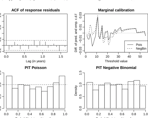
model summary and plot for diagnostic plots. The diagnostic plots like in Figure 2.2

can be produced by:

R> acf(residuals(campyfit_pois), main = "ACF of response residuals")

R> marcal(campyfit_pois, ylim = c(-0.03, 0.03), main = "Marginal calibration") R> lines(marcal(campyfit_nbin, plot = FALSE), lty = "dashed")

R> legend("bottomright", legend = c("Pois", "NegBin"), lwd = 1, + lty = c("solid", "dashed"))

R> pit(campyfit_pois, ylim = c(0, 1.5), main = "PIT Poisson")

R> pit(campyfit_nbin, ylim = c(0, 1.5), main = "PIT Negative Binomial")

0.0 0.5 1.0 1.5

−0.2

0.2

0.6

1.0

Lag (in years)

A

CF

ACF of response residuals

0 10 20 30 40 50 −0.03 −0.01 0.01 0.03 Marginal calibration Threshold value Diff

. of pred. and emp

. c.d.f

Pois NegBin

PIT Poisson

Probability integral transform

Density 0.0 0.2 0.4 0.6 0.8 1.0 0.0 0.5 1.0 1.5

PIT Negative Binomial

Probability integral transform

Density 0.0 0.2 0.4 0.6 0.8 1.0 0.0 0.5 1.0 1.5

Figure 2.2: Diagnostic plots after model fitting to the campylobacterosis data.

The response residuals are identical for the two conditional distributions. Their empirical autocorrelation function, shown in Figure 2.2 (top left), does not exhibit any serial correlation or seasonality which has not been taken into account by the models. Figure 2.2 (bottom left) points to an approximately U-shaped PIT histogram indicating that the Poisson distribution is not adequate for model fitting. As opposed to this, the PIT histogram which corresponds to the Negative Binomial distribution appears to approach uniformity better. Hence the probabilistic calibration of the Negative Binomial model is satisfactory. The marginal calibration plot, shown in Figure 2.2 (top right), is inconclusive. As a last tool we consider the scoring rules for the two distributions:

(34)

R> rbind(Poisson = scoring(campyfit_pois), NegBin = scoring(campyfit_nbin)) logarithmic quadratic spherical rankprob dawseb normsq sqerror Poisson 2.750 -0.07669 -0.2751 2.200 3.662 1.3081 16.51 NegBin 2.722 -0.07800 -0.2766 2.185 3.606 0.9643 16.51

All considered scoring rules are in favor of the Negative Binomial distribution. Based on the PIT histograms and the results obtained by the scoring rules, we decide for the Negative Binomial model. The degree of overdispersion seems to be small, as the estimated overdispersion coefficient sigmasqof 0.0297 given in the output below is close

to zero.

R> summary(campyfit_nbin) Call:

tsglm(ts = campy, model = list(past_obs = 1, past_mean = 13), xreg = interventions, distr = "nbinom")

Coefficients:

Estimate Std.Error CI(lower) CI(upper) (Intercept) 3.3184 0.7851 1.7797 4.857 beta_1 0.3690 0.0696 0.2326 0.505 alpha_13 0.2198 0.0942 0.0352 0.404 interv_1 3.0810 0.8560 1.4032 4.759 interv_2 41.9541 12.0914 18.2554 65.653 sigmasq 0.0297 NA NA NA

Standard errors and confidence intervals (level = 95 %) obtained by normal approximation.

Link function: identity

Distribution family: nbinom (with overdispersion coefficient 'sigmasq') Number of coefficients: 6

Log-likelihood: -381.1 AIC: 774.2

BIC: 791.8 QIC: 787.6

The coefficient beta_1 corresponds to regression on the previous observation, alpha_13

corresponds to regression on values of the conditional mean thirteen units back in time. The output reports the estimation of the overdispersion coefficient σ2_{, which is} related to the dispersion parameterφ of the Negative Binomial distribution byφ = 1/σ2. Accordingly, the fitted model for the number of new infections Yt in time periodt is given byYt|Ft−1 ∼NegBin(λt,33.61) with

(35)

The standard errors of the estimated regression parameters and the corresponding confidence intervals in the summary above are based on the normal approximation given in (2.6). For the additional overdispersion coefficient sigmasq of the Negative

Binomial distribution there is no analytical approximation available for its standard error. Alternatively, standard errors (and confidence intervals, not shown here) of the regression parameters and the overdispersion coefficient can be obtained by a parametric bootstrap (which takes about 15 minutes computation time on a single 3.2 GHz processor for 500

replications):

R> se(campyfit_nbin, B = 500)$se

(Intercept) beta_1 alpha_13 interv_1 interv_2 sigmasq 0.89850 0.06941 0.10136 0.93836 11.16856 0.01460 Warning message:

In se.tsglm(campyfit_nbin, B = 500) :

The overdispersion coefficient 'sigmasq' could not be estimated in 5 of the 500 replications. It is set to zero for these

replications. This might to some extent result in a biased estimation of its true variability.

Estimation problems for the dispersion parameter (see warning message) occur occasion-ally for models where the true overdispersion coefficient σ2 _{is small, i.e., which are close} to a Poisson model; see Appendix B.2. The bootstrap standard errors of the regression parameters are slightly larger than those based on the normal approximation. Note that neither of the approaches reflects the additional uncertainty induced by the model selection.

2.6.2 Road casualties in Great Britain

Next we study the monthly number of killed drivers of light goods vehicles in Great Britain between January 1969 and December 1984 shown in Figure 2.3. This time series is part of a dataset which was first considered by Harvey and Durbin (1986) for studying the effect of compulsory wearing of seatbelts introduced on 31 January 1983. The dataset, including additional covariates, is available in R in the object Seatbelts. In their paper

Harvey and Durbin (1986) analyze the numbers of casualties for drivers and passengers of cars, which are so large that they can be treated with methods for continuous-valued data. The monthly number of killed drivers of vans analyzed here is much smaller (its minimum is 2 and its maximum 17) and therefore methods for count data are to be preferred.

(36)

Time Number of casualties 0 5 10 15 1969 1971 1973 1975 1977 1979 1981 1983 1985

Figure 2.3: Monthly number of killed van drivers in Great Britain. The introduction of compulsory wearing of seatbelts on 31 January 1983 is marked by a vertical line.

For model selection we only use the data until December 1981. We choose the log-linear model with the logarithmic link because it allows for negative covariate effects. We aim at capturing the short range serial dependence by a first order autoregressive term and the yearly seasonality by a 12th order autoregressive term. Both of these terms are declared by the list element named past_obs of the argument model. Following

Harvey and Durbin (1986) we use the real price of petrol as an explanatory variable. We also include a deterministic covariate describing a linear trend. Both covariates are provided by the argument xreg. Based on PIT histograms, a marginal calibration plot

and the scoring rules (not shown here) we find that the Poisson distribution is sufficient for modeling. The model is fitted by the call:

R> timeseries <- Seatbelts[, "VanKilled"]

R> regressors <- cbind(PetrolPrice = Seatbelts[, c("PetrolPrice")], + linearTrend = seq(along = timeseries)/12)

R> timeseries_until1981 <- window(timeseries, end = 1981 + 11/12) R> regressors_until1981 <- window(regressors, end = 1981 + 11/12) R> seatbeltsfit <- tsglm(timeseries_until1981,

+ model = list(past_obs = c(1, 12)), link = "log", distr = "poisson", + xreg = regressors_until1981)

R> summary(seatbeltsfit, B = 500) Call:

tsglm(ts = timeseries_until1981, model = list(past_obs = c(1,

(37)

Coefficients:

Estimate Std.Error CI(lower) CI(upper) (Intercept) 1.7872 0.39925 1.1927 2.727 beta_1 0.0854 0.08515 -0.1055 0.209 beta_12 0.1581 0.10082 -0.0334 0.314 PetrolPrice 1.1893 2.76888 -4.0278 6.427 linearTrend -0.0306 0.00885 -0.0489 -0.016

Standard errors and confidence intervals (level = 95 %) obtained by parametric bootstrap with 500 replications.

Link function: log

Distribution family: poisson Number of coefficients: 5 Log-likelihood: -396.1 AIC: 802.2

BIC: 817.5 QIC: 802.2

Accordingly, the fitted model for the number of van driversYt killed in month t is given by Yt|Ft−1 ∼Poisson(λt) with

log(λt) = 1.9 + 0.09Yt−1+ 0.15Yt−12+ 0.08Xt−0.03t/12, t = 1, . . . ,156,

where Xt denotes the real price of petrol at time t. The estimated coefficient beta_1 corresponding to the first order autocorrelation is very small and even slightly below the size of its approximative standard error, indicating that there is no notable dependence on the number of killed van drivers of the preceding week. We find a seasonal effect captured by the twelfth order autocorrelation coefficient beta_12. Unlike in the model for the car

drivers by Harvey and Durbin (1986), the petrol price does not seem to influence the number of killed van drivers. An explanation might be that vans are much more often used for commercial purposes than cars and that commercial traffic is less influenced by the price of fuel. The linear trend can be interpreted as a yearly reduction of the number of casualties by a factor of 0.97 (obtained by exponentiating the corresponding estimated coefficient), i.e., on average we expect 2.9% fewer killed van drivers per year (which is below one in absolute numbers).

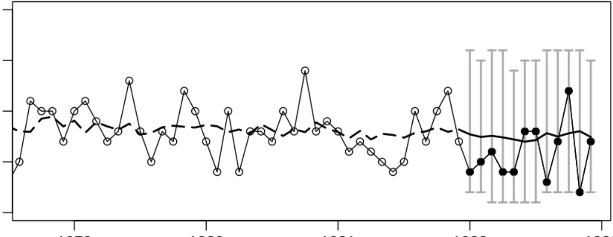
Based on the model fitted to the training data until December 1981, we can predict the number of road casualties in 1982 given the respective petrol price. Coherent, i.e. integer-valued forecasts could be obtained by rounding the predictions. A graphical representation of the following predictions is given in Figure 2.4.

R> timeseries_1982 <- window(timeseries, start = 1982, end = 1982 + 11/12) R> regressors_1982 <- window(regressors, start = 1982, end = 1982 + 11/12)