A Comparison of the Quality of Rule Induction from Inconsistent Data Sets and Incomplete Data Sets

(1)

A Comparison of the Quality of Rule Induction from

Inconsistent Data Sets and Incomplete Data Sets

By

Xiaomeng Su

Submitted to the Department of Electrical Engineering and Computer Science and the Graduate Faculty of the University of Kansas

in partial fulfillment of the requirements for the degree of Master of Science

Committee members

Jerzy W. Grzymala-Busse, Chairperson

Prasad A. Kulkarni

Zongbo Wang

(2)

The Project Report Committee for Xiaomeng Su certifies that this is the approved version of the following project report :

A Comparison of the Quality of Rule Induction from Inconsistent Data Sets and Incomplete Data Sets

Jerzy W. Grzymala-Busse, Chairperson

(3)

Abstract

In data mining, decision rules induced from known examples are used to classify unseen cases. There are various rule induction algorithms, such as LEM1 (Learning from Examples Module version 1), LEM2 (Learning from Examples Module version 2) and MLEM2 (Modified Learning from Examples Module version 2). In the real world, many data sets are imperfect, either inconsistent or incomplete. The idea of lower and upper approximations, or more generally, the probabilistic approximation, provides an effective way to induce rules from inconsistent data sets and incomplete data sets. But the accuracies of rule sets induced from imperfect data sets are expected to be lower. The objective of this project is to investigate which kind of imperfect data sets (inconsistent or incomplete) is worse in terms of the quality of rule induction. In this project, experiments were conducted on eight inconsistent data sets and eight incomplete data sets with lost values. We implemented the MLEM2 algorithm to in-duce certain and possible rules from inconsistent data sets, and implemented the local probabilistic version of MLEM2 algorithm to induce certain and possible rules from incomplete data sets. A program called Rule Checker was also developed to classify unseen cases with induced rules and measure the classification error rate. Ten-fold cross validation was carried out and the average error rate was used as the criterion for comparison. The Mann-Whitney nonparametric tests were performed to compare, separately for certain and possible rules, incompleteness with inconsistency. The re-sults show that there is no significant difference between inconsistent and incomplete data sets in terms of the quality of rule induction.

(4)

Acknowledgements

Looking back to the years I spent at KU, there are so many people who had helped me. This thesis would not have been finished without their support.

I would like to express my deepest thanks to my advisor Dr. Jerzy Grzymala-Busse for his persistent guidance on my study and thesis. His enthusiasm of teaching and research impressed me a lot, and will have long lasting effects on me. I also thank Dr. Prasad Kulkarni, Dr. Zongbo Wang for serving in my committee, and for their fantastic suggestions and inspiring questions. Thank the professors in my department for the wonderful teaching, I really learned a lot from their lectures. I’ve expanded scope of knowledge, and acquired skills for research and work in the future.

My special thanks go to Dr. Heather Desaire and Dr. Man Kong. They took care of me and were always there for me. I would not be able to sutdy here without their generous help. I also thank Pam Shadoin and Anna Paradis, for taking care of all the "little" things, but together they make a whole difference.

I am also grateful for my family and friends. They always cheer me up and stand by me through ups and downs. Thank all the people who made this report possible.

(5)

List of Figures

4.1 Experiment procedure . . . 36 4.2 Comparison of error rates of certain rules for inconsistent and incomplete data sets 38 4.3 Comparison of error rates of possible rules for inconsistent and incomplete data sets 38

(8)

List of Tables

2.1 An example of a decision table . . . 3

2.2 All attribute-value blocks of Table 2.1 . . . 4

2.3 Probabilistic approximations for[(Flu,yes)]of Table 2.1 . . . 8

2.4 An incomplete data set . . . 10

2.5 All attribute-value blocks of Table 2.4 . . . 10

2.6 Probabilistic approximations for[(Trip,yes)]of Table 2.4 . . . 14

2.7 An incomplete data set . . . 16

2.8 Probabilistic approximations for[(Hobby,f ishing)]of Table 2.7 . . . 16

3.1 A decision table for demonstrating LEM2 algorithm . . . 20

3.2 A decision table containing numerical for demonstrating MLEM2 attributes . . . . 25

3.3 An incomplete data set for demonstrating the local probabilistic version of MLEM2 algorithm . . . 30

4.1 Average error rates of inconsistent data sets . . . 37

4.2 Average error rates of incomplete data sets . . . 37

4.3 Ranking details of Mann-Whitney test to compare the error rates of certain rules induced from inconsist and incomplete data sets . . . 40

4.4 Ranking details of Mann-Whitney test to compare the error rates of possible rules induced from inconsist and incomplete data sets . . . 40

(9)

Chapter 1 Introduction

As we encounter exponential growth of data acquisition in recent years, it is of great interest to discover the hidden information lying beneath the data, so that explanation of patterns and prediction of new examples are possible. Data mining is a research area aiming to extract such previously unknown information. Classification is a type of problems in which the decision values are category labels, and the decisions of training examples are known. One way to represent the extracted knowledge of classification problems is to use decision rules.

There are many rule induction algorithms. In this project, we focused on the LERS (Learning from Examples based on Rough Set) learning system, which is a data mining system that induces a rule set from examples represented as a decision table, and classifies unseen examples using the previously induced rule set (Grzymala-Busse, 1992). LEM1 (Learning from Examples Module version 1), LEM2 (Learning from Examples Module version 2) and MLEM2 (Modified Learning from Examples Module version 2) are different rule induction algorithms frequently used in LERS system.

Ideally we want training sets to be consistent and complete, from such sets rule sets with high accuracy could be induced. However, in the real world, we usually have imperfect data sets, either inconsistent or incomplete, which make rule induction more difficult. Lower and upper approxima-tions, or more generally, probabilistic approximaapproxima-tions, provide an effective and practical way to

(10)

in-duce certain and possible rules from inconsistent data sets and incomplete data sets (Pawlak, 1982) (Pawlak, 1992) (Clark & Grzymala-Busse, 2011) Busse & Siddhaye, 2004) (Grzymala-Busse et al., 2014). The approximation is based on "indiscernibility relation", which is an equiv-alence relation on inconsistent data sets. For incomplete data set, the indiscernibility relation is reflexive, but is not necessarily symmetric or transitive. Therefore the approximation on incom-plete data set is not unique. One has several choices on which approximation to use, for example, subset approximation, concept approximation, or local approximation. However, no matter what approximation is used, the qualities of rule sets induced from inconsistent data sets and incomplete data sets are expected to be lower than rules induced from perfect data set. Since inconsistent data sets and incomplete data sets are very common, it is worth the effort to investigate which one is worse.

The objective of this project is to find out which type of imperfect data sets, inconsistent or incomplete, has more negative effects on rule induction. In this project, we implemented the conventional MLEM2 algorithm and the local probabilistic version of MLEM2 algorithm. We also developed a program to classify cases from testing set and measure the classification error rate. Experiments were carried out on eight inconsistent data sets and eight incomplete data sets. For inconsistent data sets, certain rules and possible rules were induced with MLEM2 algorithm. For incomplete data sets, we only considered one type of missing attribute values, which arelost values (denoted by ?), and applied the local probabilistic version of MLEM2 algorithm to induce certain rules and possible rules. Ten-fold cross validation was conducted on each data set, and the average error rate was used as the criterion for comparison. The Mann-Whitney nonparametric test was performed to compare, separately for certain and possible rules, incompleteness with inconsistency. The results show that inconsistent data sets and incomplete data sets are comparable with each other in terms of the quality of rule induction. There is no significant difference between the two types of imperfect data sets.

(11)

Chapter 2 Data Representation

2.1 Decision Table

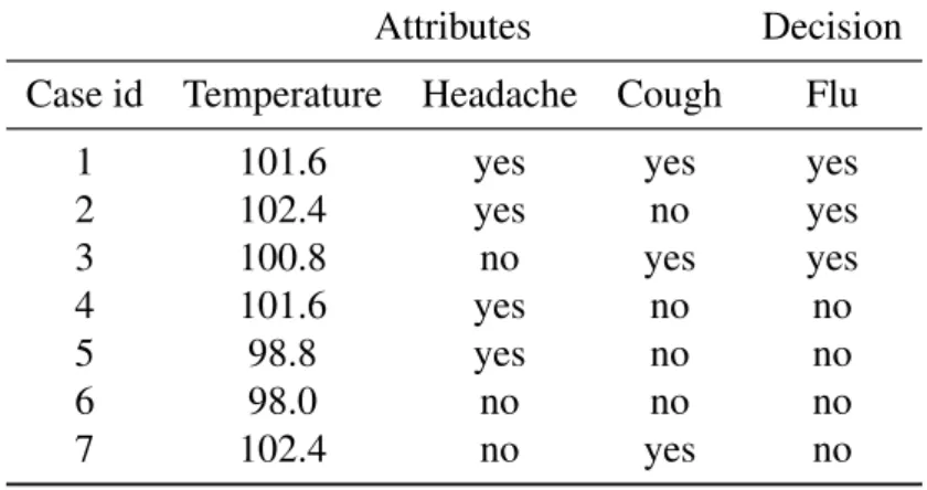
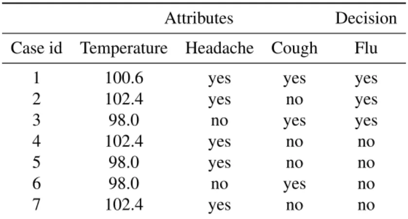
In this thesis, we follow the terminologies of the LERS system (Grzymala-Busse, 1992). In the LERS system, an input data set is presented as adecision table. Each row of a decision table is called a case, and each column corresponds to a variable. One special variable is selected as decision, and the other variables areattributes. Conventionally, we usedto denote decision,U to denote the entire set of cases, andAto denote the set of all attributes. Table 2.1 is an example of a decision table which keeps a record on the symptoms of a patient and whether he/she has flu or not. In this table,U={1,2,3,4,5,6,7},d=Flu, andA={Temperature,Headache,Cough}.

Table 2.1: An example of a decision table Attributes Decision Case id Temperature Headache Cough Flu

1 100.6 yes yes yes

2 102.4 yes no yes 3 98.0 no yes yes 4 102.4 yes no no 5 98.0 yes no no 6 98.0 no yes no 7 102.4 yes no no

(12)

Table 2.2: All attribute-value blocks of Table 2.1 (a,v) [(a,v)] (Temperature,98.0) {3,5,6} (Temperature,100.6) {1} (Temperature,102.4) {2,4,7} (Headache,yes) {1,2,4,5,7} (Headache,no) {3,6} (Cough,yes) {1,3,6} (Cough,no) {2,4,5,7}

"Headache" and "Cough" are symbolic attributes because the values of these attributes are discrete labels. On the contrary, "Temperature" is a numerical attribute because the values of this attribute are continuous numerical numbers. Numerical attributes are usually discretized to intervals. The MLEM2 algorithm handles discretization at the same time with rule induction, which will be discussed in Chapter 3.

Let adenote an attribute,x denote a case, vdenote a value of a particular attribute. The pair

(a,v) is called an attribute-value pair. For example, (Headache,yes) is an attribute-value pair. Theattribute-value pair block, denoted by[(a,v)]for complete data sets is defined as

[(a,v)] ={x|x∈U,a(x) =v} (2.1)

A full list of all attribute-value blocks of Table 2.1 is summarized in Table 2.2. Similarly, we could defineconcept, which is the block of a decision-value pair.

[(d,w)] ={x|x∈U,d(x) =w} (2.2)

In Table 2.1, there are two concepts: [(Flu,yes)] ={1,2,3}and[(Flu,no)] ={4,5,6,7}. With the knowledge of attribute-value pair blocks and concepts, we are able to discuss consistency, completeness, and approximations.

(13)

2.2 Inconsistent Data Sets

2.2.1 Indiscernibility Relation and Elementary Sets

A decision table is consistent if there does not exist more than one case that share the same values for all attributes, while belong to different concepts. A formal definition is based on indis-cernibilityrelation of cases, which is denoted by ∼

B. Let x andybe two cases and Bbe a subset

of all variables(B⊆A∪ {d}). Casex is indiscernible from case y byB if and only if for every elementainB,a(x) =a(y)(Pawlak, 1982), as is shown in Equation 2.3.

x∼ By⇔ ∀a∈B,a(x) =a(y) (2.3) In Table 2.1, we have 1∼ A1 2∼A2 2∼A4 2∼A7 3∼ A3 3∼A6 4∼A2 4∼A4 4∼A 7 5∼ A5 6∼A3 6∼A6 7∼A2 7∼A 4 7∼A7

Observe that the indiscernibility relation on a complete data set is reflexive, symmetric and transitive. In other words, the indiscernibility relation on complete data sets is an equivalence relation onU. Therefore, the idea of partition could be used to describe pairwise indiscernibility relations in a more concise way. The set of all cases that are indiscernible fromxbyB, denoted by

[x]B, is called anequivalent set.

[x]B=∩{[(a,a(x))]|a∈B} (2.4)

For example, in Table 2.1,[1]A={1}, and[2]A={2,4,7}.

PartitionB∗ofU is the set of all equivalent sets of indiscernibility relation generated byB.

(14)

IfB=A, the equivalent sets ofA∗are calledelementary sets. For Table 2.1, {Temperature}∗={{1},{2,4,7},{3,5,6}} {Headache}∗={{1,2,4,5,7},(3,6}} {Cough}∗={{1,3,6},{2,4,5,7}} {Temperature,Cough}∗={{1},{2,4,7},{3,6},{5}}

Consider two partitions onU, partitionP∗is said to be smaller than or equal to partitionQ∗if and only if for each blockE∈P∗, there exists a blockE0∈Q∗, such thatE is a subset ofE0. For example, in Table 2.1,{Temperature,Cough}∗6{Temperature}∗.

The consistency of a data set is based on the inequality of partitions. A decision table is said to beconsistentif and only ifA∗6{d}∗.

Table 2.1 is inconsistent because

A∗={Temperature,Headache,Cough}∗={{1},{2,4,7},{3,6},{5}} {d}∗={Flu}∗={{1,2,3},{4,5,6,7}}

A∗{d}∗

Note that when we discuss consistency, we assume the decision table to be complete, i.e., there are no missing attribute values. If a decision contains missing attribute values, it is categorized as incomplete data set.

2.2.2 Lower and Upper Approximations

For consistent data sets, rules for a concept could be directly induced with algorithms like LEM1 and LEM2 without preliminary processing. However, for inconsistent data sets, we need to use approximations of concepts to induce rules (Pawlak, 1992) (Grzymala-Busse, 1992). Consider an inconsistent data set, given a setX ⊆U and a setB⊆A, theB-singleton lower approximation

(15)

ofX, denoted byapprsingleton_B (X)is defined as follows

apprsingleton_B (X) ={x|x∈U,[x]B⊆X} (2.6)

TheB-subset lower approximationsofX, denoted byapprsubset_B (X)is defined as follows

apprsubset_B (X) =∪{[x]B|x∈U,[x]B⊆X} (2.7)

TheB-concept lower approximationsofX, denoted byapprconcept_B (X)is defined as follows apprconcept_B (X) =∪{[x]B|x∈X,[x]B⊆X} (2.8)

TheB-singleton upper approximationofX, denoted byapprBsingleton(X)is defined as follows

apprsingleton_B (X) ={x|x∈U,[x]B∩X 6= /0} (2.9)

TheB-subset upper approximationofX, denoted byapprsubset_B (X)is defined as follows

apprsubset_B (X) =∪{[x]B|x∈U,[x]B∩X 6= /0} (2.10)

TheB-concept upper approximationofX, denoted byapprconcept_B (X)is defined as follows

apprconcept_B (X) =∪{[x]B|x∈X,[x]B∩X6= /0} (2.11)

For example, the singleton, subset, and concept lower and upper approximations of concept

[(Flu,yes)] ={1,2,3}of Table 2.1 are

apprsingleton_A (X) =apprsubset_A (X) =apprconcept_A (X) ={1}

(16)

Table 2.3: Probabilistic approximations for[(Flu,yes)]of Table 2.1 α appr_α_,_A({1,2,3})

1/3 {1,2,3,4,6,7}

1/2 {1,3,6}

1 {1}

For inconsistent data sets, the singleton, subset and concept definitions of lower and upper approximations give the same results. Thus sometimes we could omit the word singleton, subset or concept, and simply say lower and upper approximations.

2.2.3 Probabilistic Approximations

Lower and upper approximations are special cases of a more generalized approximation called probabilistic approximation. For inconsistent data sets, the singleton, subset and concept defini-tions of probabilistic approximadefini-tions also give the same approximation results. Therefore we do not distinguish the three definitions. Given a setX ⊆U, and a setB⊆A, the probabilistic approx-imations of X with a parameterα, 0<α 61, are defined as follows (Clark & Grzymala-Busse, 2011)

apprsingleton_α_,_B (X) =apprsubset_α_,_B (X) =apprconcept_α_,_B (X) =∪{[x]B|x∈U,P(X|[x]B)>α} (2.12)

where

P(X|[x]B) = |X∩[x]B|

|[x]B| .

The probabilistic approximations of concept [(Flu,yes)] ={1,2,3} of Table 2.1 are listed in Table 2.3. Observe that with very small α, the probabilistic approximation of X equals to the B-lower approximation ofX, and with α =1 the probabilistic approximation ofX becomes the B-upper approximation ofX.

(17)

2.3 Incomplete Data Sets

2.3.1 Missing Attribute Values and Characteristic Sets

Although Table 2.1 is inconsistent, it is complete since every attribute value is specified. In the real world, there are many incomplete data sets with missing attribute values due to a lot of reasons. We consider three interpretations of missing attribute values: lostvalues, "do not care" values andattribute-conceptvalues.

• Lost values, denoted by ?

If the original value of an attribute is erased or is never obtained, we interpret it as a lost value. For lost values, we have no idea to guess what the original values are. Therefore, if a(x) =?,xis not included in any[(a,v)]blocks for all specified valuesvof attributea.

• "Do not care" values, denoted by *

"Do not care" values could be replaced by any specified values from the attribute domain. This usually happens when people do not feel comfortable to reply to some unpleasing ques-tions, like age, income, and so on. If the corresponding value of casexis "do not care" value for attributea,xis included in all[(a,v)]blocks for all specified values v of attributea.

• Attributeconcept values, denoted by

-The property of attribute-concept values lies somewhere between lost values and "do not care" values. The original attribute value is lost, but it is reasonable for us to replace it by "typical" attribute values of other cases from the same concept to which the case belongs. When computing attribute-value pair blocks, ifa(x) =-, xis included in blocks [(a,v)]for all specified valuesv∈V(x,a), where

(18)

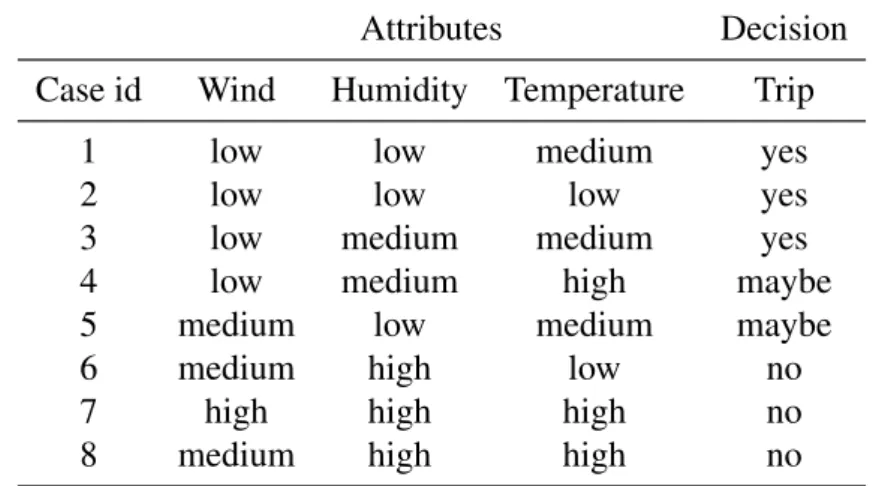
Table 2.4: An incomplete data set

Attributes Decision Case id Wind Humidity Temperature Trip

1 low low medium yes

2 - low * yes

3 * medium medium yes

4 low ? high maybe

5 medium - medium maybe

6 medium high low no

7 ? high * no

8 low low high no

Table 2.5: All attribute-value blocks of Table 2.4

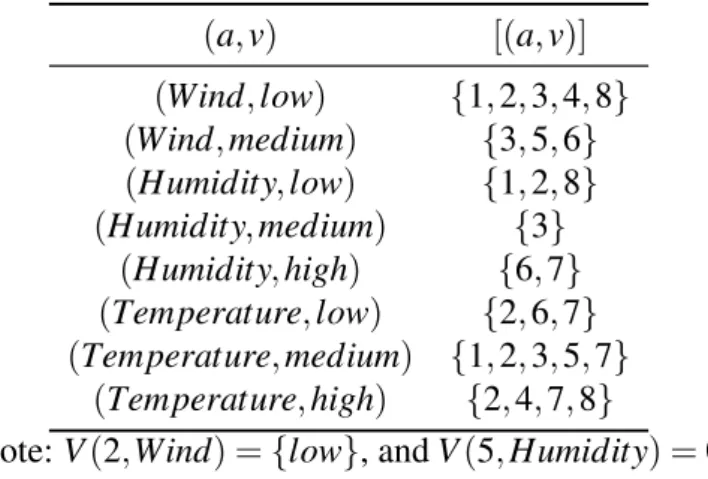
(a,v) [(a,v)] (Wind,low) {1,2,3,4,8} (Wind,medium) {3,5,6} (Humidity,low) {1,2,8} (Humidity,medium) {3} (Humidity,high) {6,7} (Temperature,low) {2,6,7} (Temperature,medium) {1,2,3,5,7} (Temperature,high) {2,4,7,8}

Note:V(2,Wind) ={low}, andV(5,Humidity) = /0

Table 2.4 is an example of an incomplete data set, and the attribute-value pair blocks of this decision table is shown in Table 2.5.

In Section 2.2.1 we have defined elementary sets for complete data sets. For incomplete data sets, the idea of elementary sets is extended to the idea of characteristic sets (Grzymala-Busse,

(19)

2004) denoted byKA. KA(x) = \ a∈A K(x,a) where K(x,a) =                  [(a,a(x)] ifa(x)is specified U ifa(x) =?, ora(x) =∗, ora(x) =- andV(x,a) = /0 S v∈V(x,a) [(a,v)] ifa(x) =- andV(x,a)6=/0 (2.14)

For the data set of Table 2.4, the characteristic sets are computed as

KA(1) ={1,2,3,4,8} ∩ {1,2,8} ∩ {1,2,3,5,7}={1,2} KA(2) ={1,2,3,4,8} ∩ {1,2,8} ∩U={1,2,8} KA(3) =U∩ {3} ∩ {1,2,3,5,7}={3} KA(4) ={1,2,3,4,8} ∩U∩ {2,4,7,8}={2,4,8} KA(5) ={3,5,6} ∩U∩ {1,2,3,5,7}={3,5} KA(6) ={3,5,6} ∩ {6,7} ∩ {2,6,7}={6} KA(7) =U∩ {6,7} ∩U={6,7} KA(8) ={1,2,3,4,8} ∩ {1,2,8} ∩ {2,4,7,8}={2,8}

Note that for incomplete data set, the indiscernibility relation is reflexive, but is not necessar-ily symmetric or transitive. Thus the indiscernibility relation on incomplete data sets is not an equivalence relation, which will make approximations not unique for incomplete data sets.

2.3.2 Lower and Upper Approximations

In Section 2.2.2, we have discussed the lower and upper approximations of concepts from an inconsistent (but complete) data set. For incomplete data sets, the lower and upper approxima-tions could be defined similarly by replacing the elementary sets by characteristic sets in all

(20)

equa-tions (Grzymala-Busse & Siddhaye, 2004). Consider an incomplete data set, given a setX ⊆U and a setB⊆A, the B-singleton lower approximationofX, denoted byapprsingleton_B (X)is defined as follows

apprsingleton_B (X) ={x|x∈U,KB(x)⊆X}. (2.15)

TheB-subset lower approximationsofX, denoted byapprsubset

B (X)is defined as follows

apprsubset_B (X) =∪{KB(x)|x∈U,KB(x)⊆X}. (2.16)

TheB-concept lower approximationsofX, denoted byapprconcept

apprconcept_B (X) =∪{KB(x)|x∈X,KB(x)⊆X}. (2.17)

TheB-singleton upper approximationofX, denoted byapprBsingleton(X)is defined as follows

apprsingleton_B (X) ={x|x∈U,KB(x)∩X 6= /0}. (2.18)

TheB-subset upper approximationofX, denoted byapprsubset

apprsubset_B (X) =∪{KB(x)|x∈U,KB(x)∩X 6= /0}. (2.19)

TheB-concept upper approximationofX, denoted byapprconcept_B (X)is defined as follows

(21)

For example, for the concept[(Trip,yes)] ={1,2,3}of Table 2.4, the approximations are apprsingleton_A (X) ={1,3} apprsubset_A (X) ={1,2,3} apprconcept_A (X) ={1,2,3} apprsingleton_A (X) ={1,2,3,4,5,8} apprsubset_A (X) ={1,2,3,4,5,8} apprconcept_A (X) ={1,2,3,8}

Observe that for incomplete data sets, the three definitions (singleton, subset and concept) of lower and upper approximations could give different results, which is different from approxima-tions on inconsistent data sets.

2.3.3 Probabilistic Approximations

Lower and upper approximations are special cases of probabilistic approximations with very small α and withα =1 respectively. Similar to the discussion in 2.2.3, we can also define the general probabilistic approximations for incomplete data sets (Grzymala-Busse et al., 2014). Given a setX ⊆U, and a setB⊆A, the probabilistic approximations ofX with a thresholdα, 0<α 61, are defined as follows

apprsingleton_α_,_B (X) ={x|x∈U,P(X|KB(x])>α} (2.21) apprsubset_α_,_B (X) =∪{KB(x)|x∈U,P(X|KB(x)>α} (2.22) apprconcept_α_,_B (X) =∪{[KB(x)|x∈X,P(X|KB(x))>α} (2.23) where P(X|KB(x)) = |X∩KB(x)| |KB(x)| .

(22)

Table 2.6: Probabilistic approximations for[(Trip,yes)]of Table 2.4

α appr_α_,_A({1,2,3}singleton) appr_α_,_A({1,2,3}subset) appr_α_,_A({1,2,3}concept)

1/3 {1,2,3,4,5,8} {1,2,3,4,5,8} {1,2,3,8}

1/2 {1,2,3,5,8} {1,2,3,5,8} {1,2,3,8}

2/3 {1,2,3} {1,2,3,8} {1,2,3,8}

1 {1,3} {1,2,3} {1,2,3}

The probabilistic approximations of concept[(Trip,yes)] ={1,2,3}of Table 2.4 are summa-rized in Table 2.6.

The singleton, subset and concept definitions of probabilistic approximations are also not unique on incomplete data sets. There is no absolute answer to the question "which definition would give the best results for rule induction". However, it is found that in many cases, if the approximation is closer to the original concept, the quality of induced rules is better. Also, it has been proved in (Clark et al., 2014) that for any conceptX and a subsetB⊆A,

apprsingleton_α_,_B (X)⊆apprsubset_α_,_B (X)

apprconcept_α_,_B (X)⊆apprsubset_α_,_B (X)

Consider thatappr_A(X)⊆X⊆appr_A(X), if one is using lower approximation for rule induc-tion, it is recommended to start with subset definiinduc-tion, and if one is using upper approximainduc-tion, concept definition might be a good choice. Singleton definition is not recommended because it may not be locally definable, which will be discussed in the next section.

2.3.4 Local approximations

In Section 2.3.3, we have mentioned that singleton approximations are not always locally defin-able. LetBbe a subset ofA, T be a set of attribute-value pairs, i.e. T ={t1,t2, ...tn},ti={ai,vi}.

If all ai are distinct and belong to B, T is called a B-complex. If B=A, we simply say T is a

complex.T is nontrivial if[T] = Tn

i=1[(ai,vi)]6= /0. A setX isglobally definableif and only ifX is a

(23)

intersections of attribute-value pair blocks from some complexes.

Definability of a set is very important because decision rules and the rule induction algorithms we are going to discuss in Chapter 3 only work on locally definable sets (Grzymala-Busse & Rzasa, 2006).

We also mentioned in 2.3.3 that usually we would like to choose an approximation that is close to the original set. Sometimes subset and concept probabilistic approximations are not satisfying. For example, consider the incomplete data set in Table 2.7, the(a,v)blocks and characteristic sets are

[(Age,under−21)] ={1,8} [(Age,21−40)] ={3,5,7}

[(Age,41−and−over)] ={4} [(Education,elementary)] ={1,3,6,8}

[(Education,secondary)] ={2,3,6,7} [(Education,higher)] ={3,4,6}

[(Gender,male)] ={1,4,8} [(Gender,f emale)] ={2,5,6,7,8}

KA(1) ={1,8} KA(2) ={2,6,7}

KA(3) ={3,5,7} KA(4) ={4}

KA(5) ={5,7} KA(6) ={2,5,6,7,8}

KA(7) ={7} KA(8) ={1,8}

The subset and concept probabilistic approximations of concept[(Hobby,f ishing)] ={1,2,3}

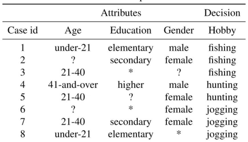
are listed in Table 2.8. If we restrict to subset and concept probabilistic approximations, we only have two choices on which approximation to use to induce rules for concept [(Hobby,f ishing)], either{1,2,3,5,6,7,8}or{1,8}. However, since any locally definable set could be expressed by a rule set, a more promising choice of approximation of concept[(Hobby,f ishing)]could be

{1,3,7,8}= [(Age,under−21)]∪([(Education,secondary)]∩[(Age,21−41)]) ={1,8} ∪({2,3,6,7} ∩ {3,5,7}).

(24)

Table 2.7: An incomplete data set

Attributes Decision Case id Age Education Gender Hobby

1 under-21 elementary male fishing

2 ? secondary female fishing

3 21-40 * ? fishing

4 41-and-over higher male hunting

5 21-40 ? female hunting

6 ? * female jogging

7 21-40 secondary female jogging 8 under-21 elementary * jogging

Table 2.8: Probabilistic approximations for[(Hobby,f ishing)]of Table 2.7 α appr_α_,_A({1,2,3}subset) appr_α_,_A({1,2,3}concept)

1/5 {1,2,3,5,6,7,8} {1,2,3,5,6,7,8}

1/3 {1,2,3,5,6,7,8} {1,2,3,5,6,7,8}

1/2 {1,8} {1,8}

1 /0 /0

Therefore, we introduce local lower approximation, local upper approximation, and local prob-abilistic approximation (Grzymala-Busse & Rzasa, 2006) (Clark et al., 2012).

• B-local lower approximation, denoted byLBX, is defined as

LBX =∪{[T]|T is a nontrivial B-complex ofX,[T]⊆X} (2.24)

For example,

L(A){6,7,8}= ([(Education,elementary)]∩[(Gender,f emale)])

∪([(Age,21−40)]∩[(Education,secondary)]∩[(Gender,male)]) ={6,7,8}

(25)

• B-local upper approximation, denoted byLBX, is defined as

LBX={[T]|∃a familyTof nontrivial B-complexes ofX,T ∈T,[T]∩X6= /0} (2.25)

Local upper approximations are not unique, for example,{6,7,8}and{1,2,6,7,8}are both local upper approximations of concept[(Hobby,jogging)].

Note:{1,2,6,7,8}= [(Age,under−21)]∪([(Education,secondary)]∩[(Gender,f emale)]).

• B-local probabilistic approximation, denoted byapprlocal

α (X), is defined as

apprlocal_α_,_B (X) =∪{[T]|∃a familyTof nontrivial B-complexes ofX,T ∈T,P(X|[T]>α)}

(2.26) Local probabilistic approximations are also not unique.

The local lower and upper approximations are special cases of the local probabilistic approxi-mation. Local approximations are very promising choices of approximations for rule induction on incomplete data sets. However, since local approximations are not unique, finding the optimal ap-proximation (i.e. the apap-proximation that is closest to the original set) is quite time consuming. One needs to examine all possible combinations of(a,v)pairs, which could not be done in polynomial time. A heuristic approach calledlocal probabilistic version of MLEM2 algorithm to calculate a single local probabilistic approximation (sub-optimal) and induce rules from incomplete data sets will be discussed in Chapter 3.

(26)

Chapter 3 Rule Induction

3.1 Decision Rules

Aruleis represented in the LERS format as shown in Equation 3.1

number1,number2,number3

(a1,v1)&(a2,v2)&(a3,v3)&. . .&(am,vm)→(d,w)

(3.1)

whereai∈A,vi∈V(ai),∀i=1,2,3, . . . ,m.

The three numbers are specificity, strength, and the rule domain size respectively, which are important features of a rule (Gryzmala-Busse & Wang, 1996).

• Specificity

The attribute-value pairs on the left-hand side of a rule are called conditions. The total num-ber of conditions indicates the complexity of a rule, which is called specificity. Specificity is usually a concern in the health and medication field, where conditions are often associated with results of lab tests. The more conditions a rule contains, the more tests a patient need to take to obtain the diagnosis.

• Rule Domain Size

(27)

we say that casex is covered by ruler. The total number of training cases that completely match the left-hand side of a rule is called the rule domain size. (The idea of training cases and testing cases are discussed in Chapter 4.) In general, we want a rule to cover as many cases as possible.

• Strength

Apart from the rule domain size, we are also interested in the correctness of a rule. The total number of training cases that are correctly classified by a rule is called strength. If all the cases that are covered by a ruler are also correctly classified byr, we say that ruleris consistent with the data set.

In most cases, a single rule only covers a few cases, thus we need a set of rules to cover as many cases in a decision table as possible. A rule setRis complete if and only if for any casei∈U, there exists a ruler, such that caseiis covered byr. A rule setRis consistent with the decision table if and only if every ruler∈Ris consistent with the decision table. The most common rule induction task is to induce a rule setRthat is both complete and consistent with the decision table.

3.2 The LEM2 Algorithm

The LEM2 (Learn from examples, module version 2) algorithm is a module of the LERS learn-ing system, which computes a local coverlearn-ing for every concept of the trainlearn-ing data set. Then the local coverings are converted to a rule set (Grzymala-Busse, 1992).

In Section 2.3.4, we have defined complexT ={t1,t2, . . . ,tn}, wheret1,t2, . . .,tnare

attribute-value pairs with distinct attribute names. Observe thatT corresponds to the left-hand side of a rule. LetBrepresent a nonempty concept or an nonempty approximation of a concert. T is aminimal complexofBif and only if (1)[T] = Tn

i=1ti⊆B; (2) There does not exist a subsetT

0_⊂_T _{such that}

[T0]⊆B. LetT={T1,T2, . . . ,Tm}be a nonempty set of nontrivial complexes.Tis alocal covering

ofBif and only if it satisfies the following conditions:

(28)

Table 3.1: A decision table for demonstrating LEM2 algorithm Attributes Decision Case id Wind Humidity Temperature Trip

1 low low medium yes

2 low low low yes

3 low medium medium yes

4 low medium high maybe

5 medium low medium maybe

6 medium high low no

7 high high high no

8 medium high high no

2. S

T∈T

T =B.

3. Tis minimal, i.e., if anyT is removed fromT, the second condition is violated.

As is mentioned earlier, a local covering could be converted to a set of rules. Condition 1 ensures that every rule in the rule set only covers cases belong toB, and every rule is as simple as possible. Condition 2 guarantees that every case inB is covered by the rule set, and condition 3 indicates that there are no redundant rules. The following example illustrates how to convert a local covering to a set of rules.

Consider a decision table as shown in Table 3.1, a local covering of concept [(Trip,yes)] =

{1,2,3}isT={{Wind,low),(Humidity,low)},{(Humidity,medium),(Temperature,medium)}}, which is corresponding to two rules for concept[(Trip,yes)]:

(Wind,low)→(Trip,yes)

(Wind,medium)→(Trip,maybe)

(Temperature,high)→(Trip,no)

The first rule covers case 1 and case 2, and the second rule covers case 3. Both rules are consistent with the data set, and there are no more cases of concept[(Trip,yes)]that are not covered by the two rules. Also, both rules are minimal because no conditions could be removed to maintain

(29)

the consistency of the rules. Furthermore, there is no redundant rule, both rules are necessary to cover all cases in [(Trip,yes)]. Similarly, we can find rules for concepts [(Trip,maybe)] and

[(Trip,no)].

Therefore, an effective way to induce a rule set from a decision table is to compute a local covering for every concept. The LEM2 algorithm is designed to find a single local covering for a given concept. The essential part of the LEM2 algorithm is to select the best attribute-value pair t from all available attribute-value pairs. Given a goal G, which is a set of cases that need to be covered, the criteria of selectingt are

1. Select at such thatt is most relevant toG. ⇔ |G∩[t]|is maximum.

2. If a tie occurs from criterion 1, select at such that the conditional probabilityP(G|[t]) is maximized.

Note that the order of the criteria brings a bonus of simplifying the computation of conditional probability. Consider P(G|[t]) = |G∩[t]|/|[t]|, the first criterion makes sure that if multiple t (t1,t2, . . . ,tk) give the same maximum relevance, we must have|G∩[t1]|=|G∩[t2]|=. . .=|G∩

[tk]|. Then smaller cardinality size of [t]results in larger value ofP(G|[t]). Thus we only need to

pick up atwith the smallest|[t]|, and it will automatically give the largestP(G|[t]).

The procedure of LEM2 is described by Algorithm 1. In this algorithm,|X|denotes the cardi-nality of setX.

Here is an example showing how the LEM2 algorithm would work on Table 3.1. First, all attribute-value pairs are computed.

[(Wind,low)] ={1,2,3,4} [(Wind,medium)] ={5,6,8}

[(Wind,high)] ={7} [(Humidity,low)] ={1,2,5}

[(Humidity,medium)] ={3,4} [(Humidity,high)] ={6,7,8}

[(Temperature,low)] ={2,6} [(Temperature,medium)] ={1,3,5}

(30)

Algorithm 1LEM2 Procedure

Input: a nonempty setB, which is a concept, or some approximation of a concept

Output: a single local coveringTof setB

1: begin procedure 2: G:=B; 3: T:= /0; 4: whileG6=0do 5: T := /0; 6: T(G):={t|[t]∩G6= /0}; 7: whileT = /0or[T]*Bdo

8: select a pairt∈T(G)such that|t∩G|is maximum; if a tie occurs, select a pairt∈T(G)

with the smallest cardinality of[t]; if another tie occurs, select first pair;

9: T :=T∪ {t}; 10: G:= [t]∩G; 11: T(G):={t|[t]∪G6= /0}; 12: T(G):=T(G)−T; 13: end while 14: foreacht∈T do 15: if[T− {t}]⊆Bthen 16: T :=T− {t}; 17: end if 18: end for 19: T:=T∪T; 20: G:=B− S T∈TT; 21: end while 22: foreachT ∈Tdo 23: if S S∈T−{T} [S] =Bthen 24: T:=T− {T}; 25: end if 26: end for 27: end procedure

(31)

Let us induce rules for concept[(Trip,yes)] ={1,2,3}. Initially,B=G={1,2,3}. The set of all relevant attribute-value pairs isT(G) ={(Wind,low),(Humidity,low),(Humidity,medium),

(Temperature,low),(Temperature,medium)}. Among all t ∈T(G), (Wind,low) yields to the maximum|t∩G|. Therefore(Wind,low)is selected andT={(Wind,low)}. SinceT *B, we have to go through another iteration of the inner while loop (lines 7 to 13 of Algorithm 1) to select the next attribute-value pair withG={1,2,3}andT(G) ={(Humidity,low),(Humidity,medium),

(Temperature,low),(Temperature,medium)}.

In the second iteration, both(Humidity,low)and(Temperature,medium)give the maximum

|t∩G|=2, and both attribute-pairs have the same cardinality of 2. We select (Humidity,low)by the heuristic of choosing first pair, thenT is updated to{(Wind,low),(Humidity,low)}. The inner while loop is terminated because[T] ={1,2} ⊆B.

Next, we need to check if T is minimal by running the first for loop (lines 14 to 18 of Algo-rithm 1), and find that no pairs could be dropped fromT. As a result,{(Wind,low),(Humidity,low)}

is the first minimal complex ofB. ThenGis updated to{3}and we identify the second minimal complex, which is {(Humidity,medium),(Temperature,medium)}. The newGis now an empty set. As we come out from the outer while loop, we need to examine ifTis minimal by running the second for loop (lines 22 to 27 of Algorithm 1). It is found that both complexes should be kept. Eventually, the local covering of concept[(Trip,yes)] ={1,2,3}is

T={{(Wind,low),(Humidity,low)},{(Humidity,medium),(Temperature,medium)}}.

3.3 Discretization and MLEM2 Algorithm

Consider some attributes like height, age, interest rate, speed and so on, usually the values of these attributes are continuous (numerical). Numerical attributes need to be discretized for rule induction. In general, there are two ways to handle data sets with numerical attributes. The first

(32)

way is to perform a preliminary discretization step, and then apply rule induction algorithms. Fre-quently used discretization methods include dominant attribute approach, multiple scanning ap-proach, and many other approaches. The second way is to include the discretization procedure into the rule induction procedure. In this project, we focus on the second approach, and adapt a mod-ified version of the LEM2 algorithm named MLEM2 for rule induction with data sets containing numerical attributes (Grzymala-Busse, 2008).

Consider an attribute a with numerical values from an interval [b,c], the discretization pro-cedure is to divide interval [b,c] into subintervals[b1,b2), [b2,b3), . . ., [bm−1,bm] where b1=b,

bm=c, andbi−i<bi,∀i=1,2,3, . . . ,m. The numbers b2, b3, . . .,bm−1are calledcut points. We

use "bi−1..bi" to represent the interval [bi−1,bi) for i<m, and use "bm−1..bm" to represent the

interval[bm−1,bm].

The MLEM2 algorithm is analogous to LEM2 in searching for best attribute-value pairs and identifying a local covering for each concept. The main difference between MLEM2 and LEM2 algorithms is the calculation of candidatest1,t2, . . ., tn (also called elementary conditions) in the

searching space. In LEM2 the elementary conditions are(a,v)pairs. In MLEM2, the elementary conditions for symbolic attributes are also(a,v)pairs, while the elementary conditions for numer-ical attributes are presented as(a,bi−1..bi), which means the value of attributeais in between of

bi−1andbi. Another difference between MLEM2 and LEM2 is the updating ofT(G)at the end of

each iteration of the inner while loop. In LEM2,T(G):=T(G)−T, which means only the selected elementary conditions are deleted from T(G). While in MLEM2, ∀t = (at,x..y)⊆T, if at is an

numerical attribute, the set{t0|t0= (at,u..v),t0⊆T(G),x..yandu..vare disjoint , orx..y⊆u..v}is

also subtracted fromT(G). This is because selectingt0won’t bring any benefit in makingT(G)a subset ofB.

Let us show how MLEM2 works using the following example. The decision table is shown in Table 3.2. There is one numerical attribute (Temperature) and two symbolic attributes (Headache and Cough). First, we calculate all the cut points for attribute "Temperature" as follows:

(33)

Table 3.2: A decision table containing numerical for demonstrating MLEM2 attributes Attributes Decision

Case id Temperature Headache Cough Flu

1 101.6 yes yes yes

2 102.4 yes no yes 3 100.8 no yes yes 4 101.6 yes no no 5 98.8 yes no no 6 98.0 no no no 7 102.4 no yes no 98.0 98.8 100.8 101.6 102.4

2. Calculate the average of two adjacent numbers, which are the cut points.

(98.0+98.8)/2=98.4 (98.8+100.8)/2=99.8

(100.8+101.6)/2=101.2 (101.6+102.4)/2=102.0

Therefore, cut points are 98.4, 99.8, 101.2, and 102.0.

Second, all elementary conditions are determined and the blocks of elementary conditions are computed. For symbolic attributes "Headache" and "Cough", the elementary conditions are attribute-value pairs. For numerical attribute "Temperature", we create two elementary conditions for every cut pointbias(Temperature,start-number..bi)and(Temperature,bi..end-number), where

start-numberis the smallest numerical value andend-numberis the largest numerical value of the attribute. The blocks of such elementary conditions are calculated as

[(a,start-number..bi)] ={x|start-number6a(x)<bi}

[(a,bi..end-number)] ={x|bi<a(x)6end-number}

Let us induce rules for concept [(Flu,yes)] ={1,2,3}. We need to identify a local covering for {1,2,3}, and the criteria of selecting the best elementary condition t are the same as in the

(34)

LEM2 algorithm. Initially,B=G={1,2,3}. All the available elementary conditions are listed as follows. [(Temperature,98.0..98.4)] ={6} [(Temperature,98.4..102.4)] ={1,2,3,4,5,7} [(Temperature,98.0..99.8)] ={5,6} [(Temperature,99.8..102.4)] ={1,2,3,4,7} (Temperature,98.0..101.2) ={3,5,6} [(Temperature,101.2..102.4)] ={1,2,4,7} [(Temperature,98..102.0)] ={1,3,4,5,6} [(Temperature,102.0..102.4)] ={2,7}

[(Headache,yes)] ={1,2,4,5} [(Headache,no)] ={3,6,7}

[(Cough,yes)] ={1,3,7} [(Cough,no)] ={2,4,5,6}

The set of all relevant attribute-value pairs is

T(G) ={(Temperature,98.4..102.4),(Temperature,99.8..102.4),

(Temperature,98..101.2),(Temperature,101.2..102.4),

(Temperature,98..102.0),(Temperature,102.0..102.4),

(Headache,yes),(Headache,no),(Cough,yes),(Cough,no)}

.

98.4..102.4)]|, the first elementary conditiont selected by MLEM2 algorithm is(Temperature,

99.8..102.4). Because [(Temperature,99.8..102.4)] = {1,2,3,4,7} *B, we need to select the next elementary condition t. To update T(G), (Temperature,99.8..102.4) should be deleted be-cause it is already selected. (Temperature,98..98.4)should also be deleted since the two intervals

[99.8,102.4]and[98,98.4)have no intersection.

The next selected elementary condition is (Cough,yes). Since[(Temperature,99.8..102.4)]∩

(35)

(Temperature,98..102.0). The first minimal complex ofBis

T ={(Temperature,99.8..102.4),(Cough,yes),(Temperature,98..102.0)}.

T is minimal, all the three elementary conditions are necessary. However,(Temperature,

99.8..102.4)and(Temperature,98..102.0)could be combined to(Temperature,99.8..102.0). The procedure of combining elementary conditions for numerical attributes is calledmerging intervals. The second minimal complex of B could be identified in a similar way, and finally we get a local covering ofBas

T={{(Temperature,99.8..102.0),(Cough,yes)},

{(Temperature,102.0..102.4),(Headache,yes)}}.

The rules for[(Flu,yes)]are

2,2,2

(Temperature,99.8..102)&(Cough,yes)→(Flu,yes)

2,1,1

(Temperature,102.0..102.4)&(Headache,yes)→(Flu,yes)

So far we only discussed how to induce rules with LEM2 and MLEM2 from consistent data sets. In Chapter 2, we discussed approximations of concepts. For inconsistent data sets and incom-plete data sets, we could apply LEM2 and MLEM2 algorithms by replacing the original concept by some approximation (e.g. lower approximation, probabilistic approximation, etc.) of the concept. Rules that are induced with lower approximations are calledcertain rules, and those induced with upper approximations are calledpossible rules.

(36)

3.4 Local Probabilistic version of MLEM2 Algorithm

We introduced local approximations for incomplete data sets. It has been mentioned that lo-cal approximations are quite promising. However, one needs to check all possible combinations of elementary conditions t to find the optimal approximation, the computation complexity is ex-ponential to the total number of t. The local probabilistic version of MLEM2 algorithm is a heuristic approach which identifies one single local approximation and induce rules at the same time (Grzymala-Busse & Rzasa, 2010). Note that the identified local approximation may not be the optimal approximation, but we are able to finish calculation in polynomial time.

The procedure of the local probabilistic version of MLEM2 algorithm (LocalPrMLEM2) is analogous to MLEM2 except for the following modifications.

1. In MELM2, we check if[T]⊆Beach time an elementary condition is selected, andBremains the same during the procedure of rule induction. While in LocalPrMLEM2, we introduce a setD, and check if[T]⊆D. Originally,D=X, andDis updated during the rule induction procedure. X is some concept.

2. For incomplete data sets, one may not get[T]⊆Dwhen one runs out of available elementary conditions. In this case, the conditional probabilityP(X|[T]) =|X∩[T]|/|[T]|is calculated. If P(X|[T]>α, thenD=D∪[T], indicating that all the cases belong to [T]are included into the approximation. Otherwise, we introduce a set of "junk complexes" J, and update J:=J∪[T], which means all the cases belong to[T]are excluded from the approximation, andT is excluded from the local coveringT.

3. When the algorithm terminates, S

S∈T

[S]represents a single local approximation ofX, andT could be converted into rules.

The full description of LocalPrMLEM2 is shown in Algorithm 2. If the input parameter α equals to 1, the algorithm induces certain rules. Ifα is very small, possible rules are induced.

To demonstrate how LocalPrMLEM2 works, let us induce rules for[(Hobby,f ishing)] ={1,2,3}

(37)

Algorithm 2Local Probabilistic version of MLEM2 Procedure

Input: a setX (a subset ofU) and a parameterα

Output: a single local probabilistic coveringTof setX

1: begin procedure 2: G:=X; D:=X; 3: T:= /0; J:= /0; 4: whileG6=0do 5: T := /0; Ts:= /0; Tn:=/0; 6: T(G):={t|[t]∩G6= /0}; 7: while(T =/0or[T]*D) and T(G)6= /0do

8: select a pairt= (at,vt)∈T(G)such that|t∩G|is maximum; if a tie occurs, select a pair

t∈T(G)with the smallest cardinality of[t]; if another tie occurs, select first pair;

9: T :=T∪ {t}; 10: G:= [t]∩G;

11: T(G):={t|[t]∪G6= /0};

12: ifat is symbolic{ letVat be the domain ofat}then

13: Ts:=Ts∪ {(at,v)|v∈Vat};

14: else

15: {at is numerical, let t = (at,u..v)} Tn := Tn∪ {(at,x..y)|disjointx..yandu..v} ∪

{(at,x..y)|x..y⊇u..v}; 16: end if 17: T(G):=T(G)−(Ts∪Tn}; 18: end while 19: ifPT(X|[T])>α then 20: D:=D∪[T]; T:=T∪ {T}; 21: else 22: J:=J∪ {T}; 23: end if 24: G:=D− S S∈T∪J [S]; 25: end while 26: foreachT ∈Tdo

27: foreach numerical attributeat with(at,u..v)∈T do

28: while(T contains at least two different pairs(at,u..v)and(at,x..y)with the same

numer-ical attributeat)do

29: replace these two pairs with a new pair(at,common part of(u..v)and(x..y));

30: end while 31: end for 32: foreacht∈T do 33: if[T− {t}]⊆Dthen 34: T :=T− {t}; 35: end if 36: end for 37: end for 38: foreachT ∈Tdo 39: if S s∈(T−{T}) [S] = S S∈T[S]then 40: T:=T− {T}; 41: end if end for 29

(38)

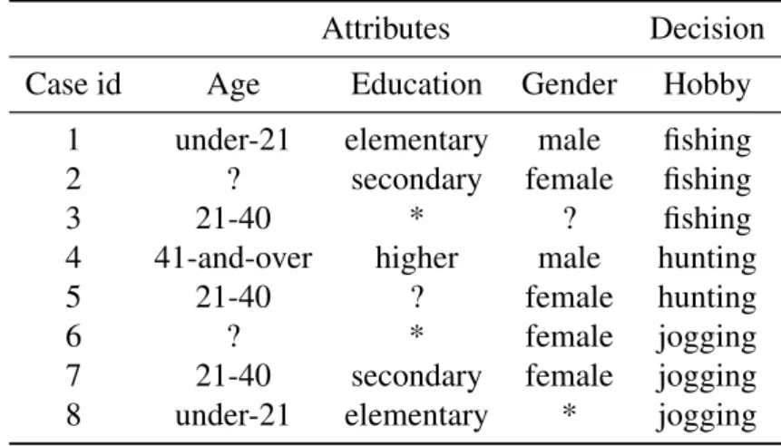
Table 3.3: An incomplete data set for demonstrating the local probabilistic version of MLEM2 algorithm

Attributes Decision Case id Age Education Gender Hobby

1 under-21 elementary male fishing

2 ? secondary female fishing

3 21-40 * ? fishing

4 41-and-over higher male hunting

5 21-40 ? female hunting

6 ? * female jogging

7 21-40 secondary female jogging 8 under-21 elementary * jogging

elementary),(Age,under−21)and(Gender,male)successively, we run out of available elemen-tary conditions and [T] = {1,8} *D. Therefore, we need to calculate the conditional proba-bility, which is P(X|[T]) = |{1,2,3} ∩ {1,8}|/|{1,8}|= 0.5. Since P(X|[T])>α, we update D:=D∪[T] ={1,2,3,8}, and

T={{(Education,elementary),(Age,under−21),(Gender,male)}}.

The new goalGbecomes {2,3}, and in a similar way we obtain the secondT as{(Education,

secondary),(Age,21−40)}and updateDto{1,2,3,7,8}.

Next, we continue to identify another T for the goal G= {2}. This time we end up with T={(Education,secondary),(Gender,f emale)}.Since[T] ={2,6,7}*D, we calculate the con-ditional probabilityP(X|[T]) =|{2}|/|{2,6,7}|=0.333. BecauseP(X|[T])<α,T is put toJand

[T] ={2,6,7}is subtracted fromG, which makes the newGto be an empty set. Then we run the for loops (lines 26 to 42 of Algorithm 2) to merge intervals and remove redundancy.

Eventually the approximation of concept [(Hobby,f ishing)] is S

S∈T[S] ={1,3,7,8}, the local

covering is

(39)

and the rules for concept[(Hobby,f ishing)]with conditional probability larger than or equal to 0.5 are

1,1,2

(Age,under−21)→(Hobby,f ishing)

2,1,2

(40)

Chapter 4 Experiments

The objective of this project is to investigate which type of data sets, inconsistent or incomplete, would have more negative effects on rule induction. In order to answer this question, we conducted experiments to induce rules from inconsistent data sets and incomplete data sets, classify testing cases with induced rules, and measure the error rate of classification. The data set from which rules are induced is called training set, and the data set on which the accuracy of classification with the induced rules is measured is called testingset. The method of classifying unseen cases is introduced in Section 4.1, the idea of ten-fold cross validation is discussed in Section 4.2. Sec-tion 4.3 described the set up and procedures of the experiments, and the results of the experiments are presented in Section 4.4.

4.1 Classification System

In this project, we followed the classification method of the LERS learning system (Gryzmala-Busse & Wang, 1996). The determination of which concept should an unseen case be classified to depends on three factors: strength, support, and partial matching factor. Strength is defined in Chapter 3 as the total number of training cases that are correctly classified by the rule. For concept C, the support ofCis defined as the sum of products of strength and specificity for all the complete

(41)

matching rules that refer to conceptC.

Support(C) =

∑

completely matching rulerdescribingC

Strength(r)×Speci f icity(r) (4.1)

If several rulesr1,r2,r3, . . . ,rn completely match a casex, and all refer to the same conceptC,

xwill be classified as a member ofC. However, if the complete matching rules refer to different concepts, supports of every concept are calculated. The conceptCwith the largest support will be the winner, andxwill be classified toC.

If complete matching is impossible for a casex, we will search for all partially matching rules. Partial matching means the attribute values of a case only match some of the conditions of a rule. Partial matching factor (pmf) is defined as the number of matched conditions divided by the total number of conditions. When complete matching is impossible, the support of conceptC is calculated as

Support(C) =

∑

partially matching rulerdescribingC

pm f(r)×Strength(r)×Sepci f icity(r) (4.2)

Again, casexis classified to the conceptCwith the largest support. For example, consider the following two cases and four rules,

Caseid Temperature Headache Cough Flu

1 high yes yes yes

(42)

2,12,15

(Temperature,high)&(Headache,yes)→(Flu,yes) (r1)

2,14,20

(Temperature,high)&(Cough,yes)→(Flu,yes) (r2)

2,16,18

(Temperature,high)&(Cough,yes)→(Flu,no) (r3)

3,20,25

(Temperature,normal)&(Headache,no)&(Cough,no)→(Flu,no) (r4)

For case 1, there are three completely matching rules r1, r2, and r3. Rulesr1 and r2 would

classify case 1 to concept[(Flu,yes)], and the support of[(Flu,yes)]is 12×2+14×2=52. Rule r3 would classify case 1 to[(Flu,no)], and the support of this concept is 16×2=32. Therefore

case 1 is classified as a member of[(Flu,yes)].

For case 2, there is no complete matching. However, we are able to find partial matching rules r1,r3andr4, with partial matching factors 0.5, 0.5 and 0.667 respectively. Ruler1refers to concept [(Flu,yes)]and the support is 12×2×0.5=12. Rulesr3 andr4refer to concept[(Flu,no)]and

the support is 16×2×0.5+20×3×0.667=56. Therefore case 2 would be classified as a member of[(Flu,no)].

4.2 Ten-fold Cross Validation

Ten-fold cross validation is commonly accepted as a standard method to measure the accuracy of classification with a rule set. In ten-fold cross validation, the data set is randomly shuffled. The re-ordered cases are divided into ten mutually disjoint subsets, and each subset contains roughly 10% cases. For each subsetSi, the other nine subsetsS1,S2, . . . ,Si−1,Si+1, . . . ,S10 are combined as

(43)

the training set for rule induction, andSi is used as the testing set. The rule set induced from the

training set is used to classify every case from the testing set, and the error rate is measured as

error_rate= number of incorrectly classified cases

number of total cases ×100% (4.3)

In total, ten runs of rule induction and classification are conducted and the average error rate is used to measure the accuracy of classification.

4.3 Experiment Procedure

We implemented the conventional MLEM2 algorithm and the local probabilistic version of MLEM2 algorithm for rule induction. We also developed a program to classify cases with induced rule sets and measure the classification error rate. Experiments were conducted on eight inconsis-tent data sets and eight incomplete data sets. The data sets were obtained by making modifications on a data set calledIris. The originalIrisdata sets contains 150 cases, 5 numerical attributes, and 3 concepts. There are no missing attribute values or inconsistent cases in the original Iris data set. Incomplete data sets were created by replacing a certain percentage of existing attribute values to lost values (denoted by ?). We obtained eight incomplete data sets, with 0%, 5%, 10%, 15%, 20%, 25%, 30%, 35% missing attribute values respectively. To set up inconsistent data sets, we discretize the data set to a point such that there were some inconsistent cases. The inconsistent data sets were discretized using a method based on agglomerative cluster analysis. Eight incon-sistent data sets were created in this way, with 6, 16, 26, 39, 49, 59, 80, and 92 inconincon-sistent cases respectively.

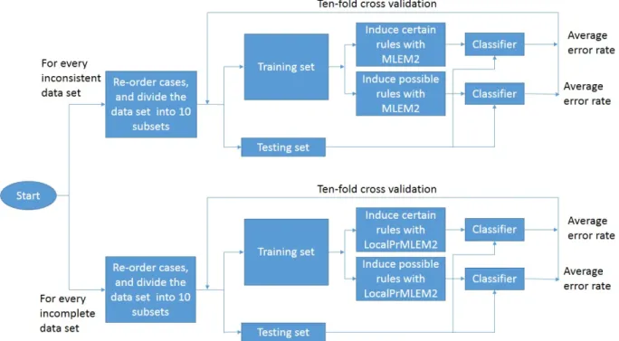
The procedure of the experiments is shown in Figure 4.1. For every inconsistent experiment data set, we applied MLEM2 algorithm to induce two sets of rules: certain rule set and possible rule set (using lower approximation and upper approximation). For every incomplete experiment data set, the local probabilistic version of MLEM2 algorithm was applied withα =1 to induce certain rules, and with α =0.0001 to induce possible rules. Ten-cross validation was conducted

(44)

Figure 4.1: Experiment procedure

to measure the average error rates of classifications with certain and possible rule sets separately. In this project, we exclude specificity (set specificity to 1) in the classification procedure, because this set up usually gives better results from previous experience (Grzymala-Busse & Zou, 1998).

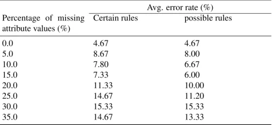
4.4 Experiment Results

The average error rates of ten-fold cross validation for inconsistent data sets are shown in Ta-ble 4.1, the percentage of inconsistency of an inconsistent data set was calculated as the ratio of the number of inconsistent cases and the number of total cases. From the table, it is observed that although there are some exceptions, the average error rates tends to be higher as the percentage of inconsistency gets larger. This conclusion holds for both certain rules and possible rules. This is because the if two inconsistent cases are covered by a rule, no matter what concept the rule refers to, at least one case is incorrectly classified. Therefore when there are many inconsistent cases, the error rate of classification is expected to be higher.