Improving unsupervised learning with exemplarCNNs

Improving Unsupervised Learning with ExemplarCNNs

Insight Centre for Data Analytics, Dublin City University

Abstract

Most recent unsupervised learning methods explore alternative objectives, often referred to as self-supervised tasks, to train convolutional neural networks without the supervision of human annotated labels. This paper explores the generation of surrogate classes as a self-supervised alternative to learn discriminative features, and proposes a clustering algorithm to overcome one of the main limitations of this kind of approach. Our clustering technique improves the initial implementation and achieves 76.4% accuracy in the STL-10 test set, surpassing the current state-of-the-art for the STL-10 unsupervised benchmark. We also explore several issues with the unlabeled set from STL-10 that should be considered in future research using this dataset.

Keywords:Unsupervised learning, self-supervised, computer vision, agglomerative clustering.

1

Introduction

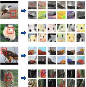
Figure 1: Examples of random transfor-mations applied to the patches extracted from the unlabeled set of STL-10

Computer vision is one of the machine learning fields most revolutionized by the successful introduction of deep learn-ing and convolutional neural networks (CNN) (Krizhevsky et al., 2012). This is not only due to technical and algo-rithmic improvements, but also due to the availability of high quality labeled datasets (Russakovsky et al., 2015; Lin et al., 2014; Everingham et al., 2012) that have allowed the exploration of new architectures and demanded a better understanding of deep learning. In parallel, the amount of data that can be collected for annotated has substan-tially increased giving the opportunity to produce even larger datasets (Li et al., 2017; Liu et al., 2016) to further explore deep learning. However, when such large amounts of data are available, the annotation process becomes very expensive and time consuming, which sometimes results in datasets with low-quality annotation, such as Clothing 1M (Liu et al., 2016) or WebVision (Li et al., 2017).

The challenge of learning from the data itself and in-dependently from the labels, known as unsupervised or

self-supervised learning, has become a key challenge in the deep learning community. The classical approaches for unsupervised learning consist of techniques like hierarchical clustering or k-means clustering, Gaussian mixture models, or self-organizing maps, and aim to extract the underlying structure in the data. In deep learning, there has been many approaches that substitute the human annotated labels by labels obtained directly from the data (Dosovitskiy et al., 2016; Zhang et al., 2016; Noroozi and Favaro, 2016) (often called self-supervised learning). These labels are created artificially from inherent properties in the data without practically any annotation cost.

In this work we propose a clustering strategy to overcome one of the main limitations of the self-supervised learning methodology proposed in (Dosovitskiy et al., 2016) (ExemplarCNN). The core idea of the method is to artificially create multiple views of different objects randomly perturbing the original image to simulate changes in the shape, lighting conditions, and camera position. This creates a surrogate dataset in which each class contains many patches from the same image (Figure 1). The model is then trained to classify the images among the surrogate classes generated. In other words, the model is trained to recognize the corrupted versions of one particular image as samples from the same category. We propose to use agglomerative clustering as a method to generate surrogate classes that contain natural variations of the objects across images.

The following section gives an overview of the current state-of-the-art in self-supervised and unsupervised learning. Section 3 provides a detailed description of the method used, the generation of the surrogate dataset, the evaluation procedure, and a discussion on some of the main challenges present in the STL-10 benchmark (Coates et al., 2011). Section 4 reports on the technical details of the experiments, show the results obtained, and provides a comparison with the relevant state-of-the-art. Finally, Section 5 presents our conclusions and outlines possible future improvements.

2

Related Work

Recent approaches for unsupervised learning focus onself-supervisedtasks, as an alternative to super-vision from manually annotated samples, where labels are automatically created directly from images (Noroozi and Favaro, 2016; Zhang et al., 2016; Dosovitskiy et al., 2016; Doersch et al., 2015; Gidaris et al., 2018). In these scenarios models are trained using alternative orpretexttasks with objectives like solving Jigsaw puzzles (Noroozi and Favaro, 2016) or colorizing images (Zhang et al., 2016).

Most self-supervised approaches are based on intuitive ideas of how humans learn visual patterns. For example, (Doersch et al., 2015) and (Noroozi and Favaro, 2016) build a task that encourages the network to understand the spatial location of certain features in the image. In (Doersch et al., 2015) the authors use two patches from the same image and train a CNN to predict the location of one patch with respect to the other. Similarly, (Noroozi and Favaro, 2016) train a model to solve Jigsaw puzzles. They argue that in this scenario, the model has to learn the different parts from the objects and that they are made of different parts. Another commonly used pretext task is colorization, a basic approach for this task is to predict the channelsabusing the information from theLchannel in theLab color space (Zhang et al., 2016). (Guadarrama et al., 2017) brings this a step further and proposes a recursive colorization to generate a high-resolution image colorization. A very simple approach is proposed in (Gidaris et al., 2018) that outperform most of the previous methods; they train a network to identify which rotation was applied to an image. Finally, (Dosovitskiy et al., 2016) propose to train a CNN to recognize patches extracted from one image as examples coming from that specific image. They extract several patches from each of the images and apply random transformations to try to replicate natural changes (location, illumination, etc). The authors explore the proposed method using the STL-10 dataset, among others. This study is especially interesting since STL-10 contains 96×96 images, which is more realistic than the commonly used lower resolution datasets (e.g. CIFAR10).

By artificially creating different views from a single image, (Dosovitskiy et al., 2016) train a CNN using stochastic gradient descent (SGD) and learn discriminative features that achieve very competitive results in several benchmarks including STL-10 and CIFAR10. There are, however, three main downsides to this method. First, this method creates a dataset where images from the same semantic class generate different surrogate classes, creating collisions and misguiding training (SGD optimization). (Dosovitskiy et al., 2016) introduce clustering methods to reduce the collisions in the datasets allowing them to increase the amount of unlabeled data used for training. Second, the method ignores the relationship between elements from the same semantic class and between elements from different classes. These two points are studied in (Bautista et al., 2016), where the authors propose a

curriculum learning approach to train the model placing samples from different classes inside every mini-batch. Third, the dataset generated with this method contains a large number of classes, which requires a very large softmax to compute the loss function and provides a weak guide for parameter updates. In (Doersch and Zisserman, 2017) the authors use a triplet loss approach to overcome this last challenge.

Other approaches step outside the unsupervised learning paradigm and try to maximally leverage the small set of labeled samples using techniques such as extreme data augmentations (DeVries and Taylor, 2017; Zhong et al., 2017), clustering techniques (Ji and Vedaldi, 2018; Dundar et al., 2015), autoencoders (Zhao et al., 2015), or other more theoretical approaches (Hjelm et al., 2019; Ji and Vedaldi, 2018). In (Hjelm et al., 2019)convolutional k-means clusteringis proposed as a technique to exploit the relationships between the layers from a deep convolutional neural network to prevent the network from learning redundant filters and learn more efficiently from less labeled data. Regarding autoencoders, (Zhao et al., 2015) propose a method where each pooling layer from the encoder generates a variable with image content information that passes to the following layer, and a variable with spatial information that passes to the corresponding layer in the decoder. (Hjelm et al., 2019) propose a more theoretical approach based on the maximization of the mutual information between the output of an encoder CNN and local regions of the input. Similarly, (Ji and Vedaldi, 2018) minimize the mutual information between the classes predicted for a pair of patches extracted of two images.

This paper proposes a method that uses agglomerative clustering to address the collisions between classes. Unlike the clustering used by Dosovitskiy et al. (2016), we use a conservative complete linkage (maximal distance) strategy to avoid clustering images from different semantic classes, eliminating the need for the heuristic of discarding noisy clusters and merging similar ones. Moreover, while the clustering proposed in Dosovitskiy et al. (2016) generates 6, 510 clusters with approximately 10 images per-cluster, we keep the number of clusters constant and equal to number of surrogate classes (16, 000), each containing approx. 4 images, thus making use of more of the unlabeled data to learn better representations.

3

Methodology

The approach used in our experiments is to generate a surrogate dataset with labels created directly from the data as an alternative to fully supervised learning. As in (Dosovitskiy et al., 2016), we extract patches from the original unlabeled data and randomly transform them to simulate different points of views of the same instance. All patches coming from the same image constitute a class from the surrogate dataset. By training a CNN to classify the transformed patches as corresponding to one or another image, the CNN learns to extract discriminative features that generalize to other tasks. We evaluated the model by extracting features from a small subset of labeled data and training a linear SVM. We then assess the accuracy of the SVM in the testing subset as specified in (Coates et al., 2011). We propose a clustering technique to improve this method and show that it allows the CNN to learn more effective representations. Our code is available athttps://git.io/fjP5u.

3.1 Surrogate dataset

We generate the surrogate dataset by extracting patches around an anchor pixel from the image and applying random transformations. The anchor pixel is selected based on its probability of being an edge. Then, we randomly translate the anchor over the horizontal and vertical axis following a random Normal distribution (a uniform distribution gives very similar results). Since the size of the resulting images is 32×32 pixels, the original image is up-scaled or down-scaled to accommodate the crops depending on the scaling factor applied to each particular patch.

Following (Dosovitskiy et al., 2016) we randomly apply several transformations from a set of transformations. We extract all patches and apply all transformations before training the CNN. The

optimal number of classes reported in (Dosovitskiy et al., 2016) is 16, 000, 100 images per class for training and 10 samples per class for validation.

We use the Sobel operator to find edges and then sample patch anchor locations with probability proportional to edge strength. The intuition here is that strong edges are prevalent near objects and other interesting image regions. Figure 1 shows examples of patches obtained after applying the transformations.

3.2 STL-10 dataset

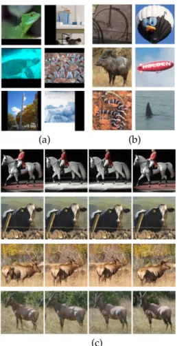
(a) (b)

(c)

Figure 2: Examples of the challenges from STL-10. a) black borders artifacts; b) out-of-distribution samples; c) near duplicates. The STL-10 benchmark (Coates et al., 2011) is an image

classification dataset designed to develop unsupervised and semi-supervised learning methodologies. It is split into train, test, and unlabeled sets. The first two are labeled sets containing 10 different categories. STL-10 im-ages were acquired from labeled ImageNet (Russakovsky et al., 2015) examples down-sampled to 96×96, which provides a challenging resolution for a benchmark of scalable unsupervised learning methods. The main mo-tivation of this benchmark is to use the unlabeled set, constituted of 100, 000 samples, to train an unsupervised model to extract features and train with a subset of 1, 000 samples from the training set (of 5, 000 images in total), and evaluate in the test subset of 8, 000 images.

3.2.1 Evaluation

We follow the testing protocol suggested in the STL-10 benchmark (Coates et al., 2011) and trained using features from the ExemplarCNN with each of the 10 predefined folds of 1, 000 samples each. We report the average and standard deviation of the accuracy of the 10 models with respect to the testing set. We followed the procedure de-scribed in (Dosovitskiy et al., 2016) to extract the features and train the one-vs-all linear SVMs: the output of each of the convolutional layers is downsampled to 2×2, flat-tened into a vector, and then concatenated all together with the output features from the fully connected layers.

3.2.2 Limitations and challenges

Exploring the data in STL-10, we found several issues regarding the unlabeled subset:

1. Images that correspond to semantic classes that are not present in the 10 classes from the labeled sets (see Figure 2b). This suggests that the use of a softmax in the final layer might be inappropriate since it adopts the closed-world assumption, which assumes that the labels of our samples are limited to the 10 classes from STL-10.

2. There are many images with artifacts such as black borders (Figure 2a). This might explain why approaches like cut-out (DeVries and Taylor, 2017; Zhong et al., 2017) are so successful in this dataset: they are learning features that are robust to artifacts very similar to those in the unlabeled set.

3. Near duplicates (see Figure 2c). We found several instances of the same image with imperceptible variations, which exacerbate one of the main limitations of ExemplarCNNs: class collisions. 3.3 Clustering

A key limitation of ExemplarCNNs is that as the number of surrogate classes increases, the number of surrogate classes created from images of the same class increases: i.e. two different surrogate classes may contain objects of the same semantic class, which provides incorrect guidance during training (SGD optimization). This is exacerbated by the fact that the unlabeled set from STL-10 has many near duplicate images that result in different surrogate classes from very similar images. These limitations motivate the application of clustering to group together similar images and palliate this effect.

We create a complete linkage hierarchical tree (dendrogram) from images in the unlabeled set from STL-10 by applying a bottom-up hierarchical clustering algorithm (hierarchical agglomerative clustering) using 50% of the unlabeled samples (randomly selected). We leave the remainder to expand the clusters after building the dendrogram. Agglomerative clustering allows specifying a maximum distance between elements in each cluster, which avoids the need to specify the number of clusters (e.g. as ink-means).

The dendrogram is created using the features from Section 3.2.1 extracted from half the unlabeled set (sampled randomly) using a CNN pretrained with the ExemplarCNN strategy. We then cut the hierarchical tree (dendrogram) to keep only the clusters where the maximum distance between images is 1.25 and obtain 2, 249 clusters of up to 7 samples each. To compare with previous results, we fix the number of surrogate classes to be generated to 16, 000. We use the clusters obtained, select the remaining classes (13, 751) from the images not used after cutting the dendrogram, and cluster each of them together with the 3 nearest images from the held-out samples in the unlabeled set (the remaining half of the data) using the cosine distance between the features extracted with the pre-trained CNN. Finally, for each image in the resulting clusters, we used the procedure described in Section 3 to generate a new surrogate dataset. Each class is generated from a cluster with an average of approximately 4 samples by extracting and transforming 100 patches for each element in the cluster.

4

Experiments

This section reports technical details of the training process, the results from our implementation of (Dosovitskiy et al., 2016), the proposed clustering methodology, and a comparison with other works from the state-of-the-art.

4.1 Training details

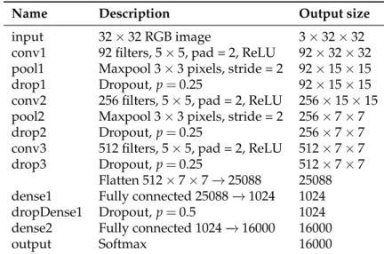
We use the 5-layer CNN proposed in (Dosovitskiy et al., 2016) that consists of 3 convolutional layers followed by 2 fully connected layers, all of them with a ReLU non-linearity. The first and the second convolutional layers are followed by max pooling with a 3×3 filter and a stride of 2. Dropout is used after every layer (p=0.25 for convolutional andp=0.5 for fully connected). Table 1 shows the structure of the network.

We use SGD to optimize the parameters of the CNN by minimizing the cross entropy loss between the softmax distribution of the output of the last layer and the surrogate class associated to each patch. Extensive experiments showed that theL2regularization and the learning rate used in this setup

considerably affects generalization. Unlike the standard configuration, this method has problems learning when all layers have the same learning rate andL2regularization weight. This is due to the

large amount of parameters in the last two layers, which is prone to overfitting. Consequently, theL2

regularization strength for the weights from the first fully connected layer is set to 0.004 and to 4 times larger (0.016) for the second fully connected layer. We do not applyL2regularization to any of the

Name Description Output size

input 32×32 RGB image 3×32×32 conv1 92 filters, 5×5, pad = 2, ReLU 92×32×32 pool1 Maxpool 3×3 pixels, stride = 2 92×15×15 drop1 Dropout,p=0.25 92×15×15 conv2 256 filters, 5×5, pad = 2, ReLU 256×15×15 pool2 Maxpool 3×3 pixels, stride = 2 256×7×7 drop2 Dropout,p=0.25 256×7×7 conv3 512 filters, 5×5, pad = 2, ReLU 512×7×7 drop3 Dropout,p=0.25 512×7×7

Flatten 512×7×7−→25088 25088 dense1 Fully connected 25088−→1024 1024 dropDense1 Dropout,p=0.5 1024 dense2 Fully connected 1024−→16000 16000

output Softmax 16000

Table 1: Structure of the CNN used in the main experiments.

biases, nor to the weights of the convolutional layers. The initial learning rate applied to the weights is 0.1 and 0.2 for the bias. However, the learning rate of the weights from the second fully connected layer is decreased to 0.025.

During training the overall initial learning rate is reduced by a factor of 0.4 in epochs 75 and 92, and by 0.25 in epochs 85 and 100. Then, the CNN is trained until epoch 110. We use a momentum of 0.9. The only pre-processing on the images during training is a per-channel normalization with the mean and standard deviation computed from the surrogate dataset generated with the transformations described in Section 3.

4.2 Clustering and ExemplarCNNs

Table 2 provides the results obtained with our implementation of ExemplarCNN together with the proposed clustering algorithm. We train an ExemplarCNN as in Section 3 and use it to extract features from STL-10 images. We then apply the clustering algorithm, generate a new surrogate dataset from the clustered images, and train from scratch following the same procedure as before.

The new clustered dataset consists of 16, 000 classes constituted by an average of approximately 4 samples each, from which we extract and transform the patches (100 patches for each image). The clustering allows us to introduce approximately 4 times the amount of data and avoid the increase of the collision that would occur if the dataset used to train the ExemplarCNN were directly increased, as reported in (Dosovitskiy et al., 2016).

Methodology Accuracy (%)

ExemplarCNN 74.14±0.39

Clustering 76.42±0.35

ImageNet 70.7±0.62 Semi-supervised 74.05

Table 2: Results from our imple-mentation evaluated in the test set from STL-10

Table 2 also reports results of some exploratory experiments. In the case ofImageNetwe used images from ImageNet to gen-erate a surrogate dataset of patches 96×96 pixels, then we train as explained in Section 4, and finally we test the features in the testing set from STL-10 following the standard procedure. The drop in accuracy can be explained due to the change of domain from ImageNet to STL-10. For the results in thesemi-supervised experiment we used the first predefined fold from the training set of STL-10, extracted the features with the ExemplarCNN, and trained a linear SVM. We then used the SVM to label all the unlabeled set from STL-10. Finally, we train a Resnet50 on the

unlabeled data with the labels predicted by the SVM and evaluate its predictions on the testing set directly. This experiment shows how ExemplarCNNs can be used as a pretext task to label unlabeled datasets and move to other approaches that address corruptions in the labels.

4.3 Comparison with the state-of-the-art

Methodology Accuracy (%)

SWWAE (Zhao et al., 2015) 74.3 ConvClustering (Dundar et al., 2015) 74.10 ExemplarCNN (Dosovitskiy et al., 2016) 74.2±0.4

ExemplarCNN (ours) 74.14±0.39

Clustering (ours) 76.42±0.35

Cutout* (DeVries and Taylor, 2017) 87.26 IIC* (Ji and Vedaldi, 2018) 88.8

Table 3: Comparison with the state-of-the-art. The meth-ods marked with * use the full training set from STL-10. Table 3 compares the current

state-of-the-art results for STL-10. Our clustering tech-nique, that uses only one of the 10 pre-defined folds from STL-10 for the testing stage, achieves the highest performance compared to the methods that use the pre-defined folds. The methods that ignore the predefined fold from STL-10 focus on show-ing how to use few labels to learn better rep-resentations, while in this work we focus on learning representations from unlabeled data and use them as a prior to train in a very small amount of labeled data. We

marked with a star (*) the works that used the full training set from STL-10, which implies training with 5, 000 labels instead of the 1, 000 from the predefined folds proposed as the the STL-10 benchmark. This difference can be appreciated in the results: the works that use all the training set report accuracies that are up to 12% above the best performance of the approaches that use only 1, 000 labeled samples.

5

Conclusions and future work

This paper proposed a clustering technique that complements the self-supervised learning methodol-ogy from (Dosovitskiy et al., 2016) to overcome the increase of collisions between surrogate classes when the amount of unlabeled data used is increased. This method learns discriminative representa-tions without supervision from human annotarepresenta-tions and achieves state-of-the-art performance in the STL-10 unsupervised benchmark. In addition we provide an insight on the limitations and challenges that the STL-10 dataset present.

Acknowledgments

We thank Diego Ortego for valuable suggestions that helped to improve this paper. This work was supported by Science Foundation Ireland (SFI) under grant numbers SFI/15/SIRG/3283 and SFI/12/RC/2289.

References

Bautista, M. A., Sanakoyeu, A., Tikhoncheva, E., and Ommer, B. (2016). Cliquecnn: Deep unsupervised exemplar learning. InAdvances in Neural Information Processing Systems, pages 3846–3854.

Coates, A., Ng, A., and Lee, H. (2011). An analysis of single-layer networks in unsupervised feature learning. InProceedings of the Fourteenth International Conference on Artificial Intelligence and Statistics, volume 15 ofProceedings of Machine Learning Research, pages 215–223, Fort Lauderdale, FL, USA. PMLR.

DeVries, T. and Taylor, G. W. (2017). Improved regularization of convolutional neural networks with cutout. arXiv preprint arXiv:1708.04552.

Doersch, C., Gupta, A., and Efros, A. A. (2015). Unsupervised visual representation learning by context prediction. InProceedings of the IEEE International Conference on Computer Vision, pages 1422–1430.

Doersch, C. and Zisserman, A. (2017). Multi-task self-supervised visual learning. InProceedings of the IEEE International Conference on Computer Vision, pages 2051–2060.

Dosovitskiy, A., Fischer, P., Springenberg, J. T., Riedmiller, M., and Brox, T. (2016). Discriminative unsupervised feature learning with exemplar convolutional neural networks. IEEE transactions on pattern analysis and machine intelligence, 38(9):1734–1747.

Dundar, A., Jin, J., and Culurciello, E. (2015). Convolutional clustering for unsupervised learning. CoRR, abs/1511.06241.

Everingham, M., Van Gool, L., Williams, C. K. I., Winn, J., and Zisserman, A. (2012). The PASCAL Visual Object Classes Challenge 2012 (VOC2012) Results.

Gidaris, S., Singh, P., and Komodakis, N. (2018). Unsupervised representation learning by predicting image rotations. InInternational Conference on Learning Representations.

Guadarrama, S., Dahl, R., Bieber, D., Shlens, J., Norouzi, M., and Murphy, K. (2017). Pixcolor: Pixel recursive colorization. InBritish Machine Vision Conference 2017, London, UK, September 4-7, 2017. Hjelm, R. D., Fedorov, A., Lavoie-Marchildon, S., Grewal, K., Bachman, P., Trischler, A., and Bengio,

Y. (2019). Learning deep representations by mutual information estimation and maximization. In International Conference on Learning Representations.

Ji, Xu, F. H. J. and Vedaldi, A. (2018). Invariant information clustering for unsupervised image classification and segmentation. arXiv preprint arXiv:1807.06653.

Krizhevsky, A., Sutskever, I., and Hinton, G. E. (2012). Imagenet classification with deep convolutional neural networks. InAdvances in neural information processing systems, pages 1097–1105.

Li, W., Wang, L., Li, W., Agustsson, E., and Van Gool, L. (2017). Webvision database: Visual learning and understanding from web data. arXiv preprint arXiv:1708.02862.

Lin, T.-Y., Maire, M., Belongie, S., Hays, J., Perona, P., Ramanan, D., Dollár, P., and Zitnick, C. L. (2014). Microsoft coco: Common objects in context. InEuropean conference on computer vision, pages 740–755. Springer.

Liu, Z., Luo, P., Qiu, S., Wang, X., and Tang, X. (2016). Deepfashion: Powering robust clothes recognition and retrieval with rich annotations. InProceedings of IEEE Conference on Computer Vision and Pattern Recognition (CVPR).

Noroozi, M. and Favaro, P. (2016). Unsupervised learning of visual representations by solving jigsaw puzzles. InEuropean Conference on Computer Vision, pages 69–84. Springer.

Russakovsky, O., Deng, J., Su, H., Krause, J., Satheesh, S., Ma, S., Huang, Z., Karpathy, A., Khosla, A., Bernstein, M., Berg, A. C., and Fei-Fei, L. (2015). ImageNet Large Scale Visual Recognition Challenge. International Journal of Computer Vision (IJCV), 115(3):211–252.

Zhang, R., Isola, P., and Efros, A. A. (2016). Colorful image colorization. InEuropean conference on computer vision, pages 649–666. Springer.

Zhao, J. J., Mathieu, M., Goroshin, R., and LeCun, Y. (2015). Stacked what-where auto-encoders.CoRR, abs/1506.02351.

Zhong, Z., Zheng, L., Kang, G., Li, S., and Yang, Y. (2017). Random erasing data augmentation. arXiv preprint arXiv:1708.04896.