Scheduling for Multi-Core Processors
∗
Viet Anh Nguyen
1, Damien Hardy
2, and Isabelle Puaut
31 University of Rennes 1/IRISA, Rennes, France
2 University of Rennes 1/IRISA, Rennes, France
3 University of Rennes 1/IRISA, Rennes, France
Abstract
Most schedulability analysis techniques for multi-core architectures assume a single Worst-Case Execution Time (WCET) per task, which is valid in all execution conditions. This assumption is too pessimistic for parallel applications running on multi-core architectures with local instruction or data caches, for which the WCET of a task depends on the cache contents at the beginning of its execution, itself depending on the task that was executed before the task under study.
In this paper, we propose two scheduling techniques for multi-core architectures equipped with local instruction and data caches. The two techniques schedule a parallel application modeled as a task graph, and generate a static partitioned non-preemptive schedule. We propose an optimal method, using an Integer Linear Programming (ILP) formulation, as well as a heuristic method based on list scheduling. Experimental results show that by taking into account the effect of private caches on tasks’ WCETs, the length of generated schedules is significantly reduced as compared to schedules generated by cache-unaware scheduling methods. The observed schedule length reduction on streaming applications is 11% on average for the optimal method and 9% on average for the heuristic method.
1998 ACM Subject Classification C.3 Real-Time and Embedded Systems
Keywords and phrases real-time scheduling, cache-conscious scheduling, many-core architec-tures, ILP, static list scheduling
Digital Object Identifier 10.4230/LIPIcs.ECRTS.2017.14
1
Introduction
Many-core platforms are increasingly used to execute high performance hard real-time applications since they provide enough computing power to satisfy the applications’ demand while reducing their size, weight, and power requirements. However, guaranteeing the real-time constraints of safety-critical parallel applications on such platforms is quite challenging. One important challenge is to precisely estimate the Worst-Case Execution Times (WCETs) of codes executing on multi-cores. Many WCET estimation methods have been designed in the past for single-core architectures [34]. Such techniques take into account both the program paths and the core micro-architecture. Extending them to multi-core architectures is challenging, because some hardware resources, such as caches or buses are
∗ This work was supported by PIA project CAPACITES (Calcul Parallèle pour Applications Critiques en
Temps et Sûreté), reference P3425-146781.
T2 (DFT) (DFT) T3 (DFT) T4 (DFT) T5 T6 (Com-bine) T7 (Com-bine) T8 (Com-bine) T9 (Com-bine) T10 (Com-bine) T13 (Com-bine) T12 (Com-bine) T11 (Com-bine) T1 (Splitt -er) T14 (Out) Entry task Exit task
Figure 1Task graph of a parallel version of a 8-input Fast Fourier Transform (FFT) application [2].
shared between cores, which makes the WCET of a task dependent on the tasks executing on the other cores [20, 10]. Additionally, on architectures with local caches, the WCET of a task depends on the cache contents when the task starts executing, which depends on the scheduling strategy. The WCET of one task is thus no longer unique. It depends on the execution context of the task (tasks executed before it, concurrent tasks), the execution context being defined by the scheduling strategy. We thus believe that scheduling strategies that are aware of the multi-core hardware (in particular local caches) have to be defined.
Many multi-core scheduling strategies assume a single context-insensitive WCET per task. In this paper, we propose insteadcache-awarescheduling strategies, that take benefit of cache reuse between tasks. Each task has distinct WCET values depending on which other task has been executed before it on the same core (WCETs are context-sensitive). The proposed scheduling strategies map tasks on cores and schedules tasks on cores; the objective is to account for cache reuse to obtain the shortest schedules. For the scope of this paper, we focus on a single parallel application, modeled as a task graph, in which nodes represent tasks and edges represent dependence relations between them.
To further motivate our work, let us consider, as an example, a 8-input Fast Fourier Transform application. Its task graph is shown in Figure 1. This application contains both code and data reuse between tasks. For instance, T2 and T3 feature code reuse since they call the same function, and T2 and T6 feature data reuse since the output of T2 is the input of T6. On that example, we observe a WCET reduction of 10.7% on average when considering the cache affinity between pairs of tasks that may execute consecutively on the same core. The schedule length for that parallel application was reduced by 8% by using the Integer Linear Programming (ILP) technique presented in Section 4.1 as compared to its cache-agnostic equivalent.
In this paper, we propose two different methods to determine a static partitioned non-preemptive schedule aiming at minimizing the schedule length, for a parallel application by taking into account the variation of tasks’ WCETs due to reuse of code and data between tasks. The first method is based on an Integer Linear Programming (ILP) formulation and produces optimal schedules. The second method is a heuristic technique that produces schedules very fast with schedule lengths close to the optimal ones.
The main contributions of our work are as follows:
We argue and experimentally validate the importance of addressing the effect of private caches on tasks’ WCETs in scheduling.
We propose an ILP-based scheduling method and a heuristic scheduling method to statically find a partitioned non-preemptive schedule of a parallel application modeled as a directed acyclic graph.
We provide experimental results showing, among others, that the proposed scheduling techniques result in shorter schedules than their cache-agnostic equivalent.
The rest of this paper is organized as follows. Section 2 surveys related work. Section 3 describes our system model and formulates the scheduling problem. Section 4 introduces the proposed ILP formulation and the proposed heuristic scheduling method. We experimentally evaluate our proposed scheduling methods in Section 5. Finally, we summarize the contents of the paper and provide directions for future work in Section 6.
2
Related work
Schedulability analysis techniques rely on the knowledge of the Worst-Case Execution Times of tasks. Originally designed for single-core processors, static WCET estimation techniques were extended recently to cope with multi-core architectures. Most research have focused on modeling shared resources (e.g., shared cache, shared bus, shared memory) in order to capture interferences between tasks which execute concurrently on different cores [15, 18, 6, 28, 13, 1]. Most extensions of WCET estimation techniques for multi-cores produce a WCET for a single task in the presence of concurrent executions on the other cores. By construction, those extensions do not account for caches effects between tasks as our scheduling techniques do. The scheduling techniques we propose have to rely on WCET estimation techniques to estimate the effect of local caches on tasks’ WCETs.
Some WCET estimation techniques pay attention to the effect of private caches on WCETs. In [21], when analyzing the timing behavior of a task, Nemer et al. take into account the set of memory blocks that has been stored in the instruction cache (by the execution of previous tasks on the same core) at the beginning of its execution. Similarly, Potop-Butucaru and Puaut [26], assuming task mapping on cores known, jointly perform cache analysis and timing analysis of parallel applications. These two WCET estimation techniques assume task mapping on core and task schedule on each core known. In this paper, in contrast, task mapping and scheduling are selected to take benefit of cache reuse to have the shortest possible schedule length.
Much research effort has been spent on scheduling for multi-core platforms. Research on real-time scheduling for independent tasks is surveyed in [7]. This survey gives a taxonomy of multi-core scheduling strategies: global vs. partitioned vs. semi-partitioned, preemptive vs. non preemptive, time-driven vs. event-driven. The scheduling techniques we propose in this paper generate offline time-driven non-preemptive schedules. Most of the scheduling strategies surveyed in [7] are unaware of the hardware effects and consider a fixed upper bound on tasks’ execution times. In contrast, the scheduling techniques we propose in this paper address the effect of private caches on tasks’ WCETs. Our work integrates this effect in the scheduling and mapping problem by considering multiple WCETs for each task depending on their execution contexts (i.e. cache contents at the beginning of their execution).
Some scheduling techniques that are aware of hardware effects were proposed in the past. They include techniques that simultaneously schedule tasks and the messages exchanged between them [5, 30, 27]; such techniques take into consideration the Network-On-Chip
CPU I$
Shared memory
Core 1 Core 2 Core n
… D$ CPU I$ D$ CPU I$ D$ Bus
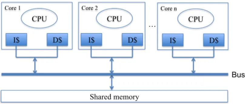
Figure 2Considered multi-core architecture.
(NoC) topology in the scheduling process. Some other techniques aim at scheduling tasks in a way that minimizes the contentions when accessing shared resources (e.g., shared bus, shared caches) [4, 11, 9]. Besides, some approaches [35, 3, 23, 22, 24] schedule tasks according to execution models that guarantee temporal isolation between co-running tasks. In that way, scheduled tasks are guaranteed to be free from the contentions when accessing shared resources. In [29], Suhendra et al. consider data reuse between tasks to perform task scheduling for multi-core systems equipped with scratchpad memory (SPM); in their work, the most frequently accessed data are allocated in SPM to reduce the accesses latency to an off-chip memory. Our scheduling solutions in this paper differ from the above-mentioned previous works because we pay attention to the effect of private caches on tasks’ WCETs. In our proposed scheduling methods, tasks are scheduled to get benefit from the effect of private caches.
Related studies also address the effect of private caches when scheduling tasks on multi-core architectures [33, 25, 31]. However, they are based on global and preemptive scheduling techniques, in which the cost of cache reload after being preempted or migrated has to be accounted for. Compared to these works, our technique is partitioned and non preemptive. We believe such a scheduling method allows to have better control on cache reuse during scheduling. Furthermore, [25] and [31] focus on single core architectures while our work target multi-core architectures.
3
System model and problem formulation
3.1
Hardware model
The class of architectures addressed in this work is the class of identical multi-core architec-tures, in which each core is equipped with a private instruction cache and a private data cache, as illustrated in Figure 2.
Clocks of all cores are assumed to be synchronized. Furthermore, it is assumed that the architecture is either (preferably) free from contention to access shared resources (shared bus, shared memory) or provides a way to bound the cost of interference, and in that latter case the cost of interference is included in tasks’ WCETs. The issue of hardware resource sharing is thus considered outside the scope of this paper.
3.2
Task and execution model
Each application is modeled as a Directed Acyclic Graph (DAG) [16], as previously illustrated in Figure 1. A node in the DAG represents a task, denotedτi. An edge in the DAG represents
a precedence relation between the source and target tasks, as well as possibly a transfer of information between them. A task can start executing only when all its direct predecessors have finished their execution, and after all data transmitted from its direct predecessors are available. A task with no direct predecessor is anentry task, whereas a task with no direct successor is anexit task. Without loss of generality it is assumed that there is a single entry task and a single exit task per application.
The structure of the DAG is static, with no conditional execution of nodes. The volume of data transmitted along edges (possibly null) is known offline. Each task in the DAG is assigned a distinct integer identifier.
A communication for a given edge is implemented using transfers to and from a dedicated buffer located in shared memory. To simplify the description of the scheduling algorithms, the worst-case communication cost for a given edge is assumed constant, and is integrated in the WCETs of the sending and receiving tasks. However, we believe that non constant communication costs (e.g. depending on task mapping), could be easily integrated in the proposed scheduling algorithms.
Due to the effect of caches, each task τj is not characterized by a single WCET value
but instead by a set of WCET values. The most pessimistic WCET value for a task, noted
W CETτj, is observed when there is no reuse of cache contents loaded by a task executed immediately beforeτj. A set of WCET values notedW CETτi→τj represent the WCETs of taskτj whenτj reuses some information, loaded in the instruction and/or data cache by a
taskτi that is executed immediately beforeτj on the same core.
3.3
Problem formulation
Our proposed scheduling methods take as inputs the number of cores of the architecture and the DAG of a parallel application decorated with WCET information for each task, and produce an offline time-driven partitioned non-preemptive schedule of the application. More precisely, the produced schedule for each core determines the start and finish times of all tasks assigned to the core.
4
Cache-conscious task scheduling methods
For solving the formulated scheduling problem, we propose two methods:
An ILP formulation that allows to reach the optimal solution, i.e. the one that minimizes the application schedule length) (see Section 4.1);
A heuristic method, based on list scheduling, that allows to find a valid schedule very fast and generally very close to the optimal one (see Section 4.2).
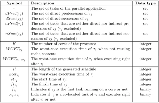
The notations used in the description of the scheduling methods are summarized in Table 1. The first block defines frequently used notations to manage the task graph. The second block defines integer constants, using upper case letters, used throughout the paper. Finally, the third block defines the variables, using lower case letters, used in the ILP formulation.
4.1
Cache-conscious ILP formulation (CILP)
In this section, we present the cache-conscious ILP formulation, noted CILP (for Cache-conscious ILP) hereafter. As mentioned before, one output of the scheduling methods is the mapping of tasks on cores. Since cores are identical, theexact core onto which a task is mapped does not matter. Based on that observation, CILP focuses on finding the sets
Table 1Notations used in the proposed scheduling methods.
Symbol Description Data type
τ The set of tasks of the parallel application set
dP red(τj) The set of direct predecessors ofτj set
dSucc(τj) The set of direct successors ofτj set
nP red(τj) The set of tasks that are neither direct nor indirect
pre-decessors ofτj (τjexcluded)
set nSucc(τj) The set of tasks that are neither direct nor indirect
suc-cessors ofτj (τj excluded)
set
K The number of cores of the processor integer
W CETτj The worst-case execution time of τj when not reusing
cache contents
integer W CETτi→τj The worst-case execution time ofτjwhen executing right
afterτi
integer
sl The length of the generated schedule integer
wcetτj The worst-case execution time ofτj integer
stτj The start time ofτj integer
f tτj The finish time ofτj integer
fτj Indicates ifτj is the first task running on a core or not binary
oτi→τj Indicates ifτjis a co-located task ofτiand executes right
afterτior not
binary
of co-located tasks with their running orders. The assignment of sets of co-located tasks to cores is then straightforward (i.e. one set per core).
The objective function of CILP is to minimize the schedule length sl of the parallel application which is expressed as follows:
minimize sl (1)
Since the schedule length for the parallel application has to be larger than or equal to the finish timef tτj of any task τj, the following constraint is introduced:
∀τj∈τ,
sl≥f tτj
(2) The finish timef tτj of a taskτj is equal to the sum of its start timestτj and its worst case execution timewcetτj:
∀τj∈τ,
f tτj =stτj +wcetτj
(3) In the above equation, variable wcetτj is introduced to model the variations of tasks’ WCETs due to the effect of private caches and is computed as follows:
∀τj ∈τ,
wcetτj =fτj∗W CETτj +
X
τi∈nSucc(τj)
oτi→τj∗W CETτi→τj
(4)
The left part corresponds to the case where taskτj is the first task running on a core
(fτj = 1). The sum in the right part corresponds to the case where the taskτj is scheduled just after another co-located taskτi (oτi→τj = 1). As shown later, only one binary variable amongfτj and variablesoτi→τj will be set by the ILP solver, thus assigning one and only one of the WCET values toτj depending on which other task is executed before it.
Constraints on tasks’ start times
A task can be executed only when all of its direct predecessors have finished their execution. In other words, its start time has to be larger than or equal to the finish times of all its direct predecessors.
∀τj∈τ,∀τi∈dP red(τj),
stτj ≥f tτi if dP red(τj)6=∅
stτj ≥0 otherwise
(5)
In the above equation, when the task has no predecessor, its start time has to be larger than or equal to zero.
Furthermore, in case there is a co-located task τi scheduled right before τj, τj cannot
start before the end ofτi. In other words, the start time ofτj has to be larger than or equal
to the finish time ofτi. Note that,τj can be scheduled only after a taskτi that is neither its
direct nor indirect successor. ∀τj ∈τ,∀τi∈nSucc(τj),
stτj ≥oτi→τj∗f tτi
(6)
For linearizing equation (6), we use the classical big-M notation which is expressed as: ∀τj ∈τ,∀τi∈nSucc(τj),
stτj ≥f tτi+ (oτi→τj −1)∗M
(7)
whereM, is a constant1higher than any possiblef tτj. Constraints on tasks’ ordering
A task has at most one co-located task scheduled right after it, which is expressed as follows:
∀τj∈τ, if nP red(τj)6=∅ X
τi∈nP red(τj)
oτj→τi≤1.
(8)
Note that, taskτj can be only scheduled before taskτiwhich is neither its direct nor indirect
predecessor.
Furthermore, a task has one co-located task scheduled right before it which is neither its direct nor indirect successor or it is the first scheduled task, thus:
∀τj ∈τ, X
τi∈nSucc(τj)
oτi→τj+fτj = 1.
(9)
Finally, since the number of cores is K, the number of tasks that can be the first to be scheduled on cores is at most K:
X
τj∈τ
fτj ≤K . (10)
1 For the experiments,M is the sum of all tasks’ WCETs when not reusing cache contents, to ensure that
The result of the mapping/scheduling problem after being solved by an ILP solver is then defined by two sets of variables. Task mapping is defined by variablesfτj andoτi→τj that altogether define the set of co-located tasks and their execution order. The static schedule on every core is defined by variablesstτj andf tτj, that define the start and finish time of the tasks assigned to that core.
4.2
Cache-conscious list scheduling method (CLS)
Finding an optimal schedule for a partitioned non-preemptive scheduling problem is NP-hard [14]. Therefore, we developed a heuristic scheduling method that efficiently produces schedules that are close to the optimal ones. The proposed heuristic method is based on list scheduling (see [17] for a survey of list scheduling methods).
The proposed heuristic method (CLS, for Cache-conscious List Scheduling) first constructs a list of tasks to be scheduled. Then, the list of tasks is scanned sequentially, and each task is scheduled without backtracking. When scheduling a task, all cores are considered for hosting the task and a schedule that respects precedence constraints is constructed for each. The core which allows the earliest finish time of the task is selected and the corresponding schedule is kept.
The ordering of the tasks in the list has to follow topological ordering such that precedence constraints are respected. Here, we select a topological order that also takes into account the WCETs of tasks. Since a task may have different WCETs according to the other task executed before it, we associate to each task aweight that approximates its WCET variation. The weight of a taskτj, notedtwτj, is defined as follows:
twτj = 1
K ∗minτi∈nSucc(τj)(W CETτi→τj) + (1− 1
K)∗W CETτj. (11) This formula integrates the likeliness that the WCET of taskτjis reduced, which decreases
when the number of cores increases. Different definitions of tasks weights were tested to take into account the WCET variation of tasks. Since we did not observe major difference between them, we selected this simple definition.
Given tasks’ weights, the order of tasks in the list is determined based on two classical metrics, both respecting topological order. The first metric is called in the followingbottom level. It defines for taskτj the longest path fromτjto the exit task (τj included), cumulating
tasks’ weights along the path:
bottom_levelexit=twexit
bottom_levelτj =max(bottom_levelτi+twτj),∀τi ∈dSucc(τj) (12) The second metric is called top level. Symmetrically, it defines for taskτj the longest
path from the entry task toτj (τj excluded):
top_levelentry= 0
top_levelτj =max(top_levelτi+twτi),∀τi∈dP red(τj) (13) As it will be shown in Section 5.2 none of the two metrics was shown to outperform the other for all task graphs, we thus kept both variations. In the following:
CLS_BL refers to a sorting of tasks according to their bottom levels; in case of equality, their top levels is used to break ties; if a tie still exists, the task identifier is used to sort tasks.
CLS_TL refers to a sorting of tasks according to their top levels, with bottom level and task identifier as tie breaking rules.
CLS refers to the method, among CLS_BL and CLS_TL, resulting in the shortest schedule length for a given task graph.
T1
T2 T3 T4
T5
τj
τi
T1 T2 T3 T4 T5 Weight Bottom Level
T1 10 – – – – 10 42.5
T2 15 20 10 20 – 15 27.5
T3 20 15 25 25 – 20 32.5
T4 15 20 20 20 – 17.5 30
T5 15 10 10 10 15 12.5 12.5
Figure 3Illustrative example for CLS_BL.
T1 T3 T4 T2 T5 T3 T4 T2 T5 T4 T2 T5 T2 T5 T5 T1 T1 T3 T4 T1 T3 T1 T3 T4 T2 T1 T3 T2 T4 T5
Core 1 Time (cycles)
Core 2 Core 1 Core 2 Core 1 Core 1 Core 1 Core 2 Core 2 Core 2 List 0 10 0 10 30 0 10 30 10 30 0 10 30 40 10 30 0 10 30 40 50 10 30 Figure 4Illustration of CLS_BL.
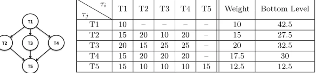
We illustrate the execution of CLS_BL on a very simple task graph whose characteristics are given in Figure 3. The left part of Figure 3 gives the task graph. The right part gives the WCETs of tasks when not reusing cache contents (W CETτj, diagonal of the left part of the table) and values ofW CETτi→τj; the next two columns give the weights and the bottom levels of tasks.
The execution of CLS_BL is illustrated in Figure 4 for a dual-core architecture. First, the tasks are ordered in a list according to their bottom levels. Then, the task at the head of the list (T1) is scheduled and T1 is removed from the list. Here, T1 is assigned to the first core. Next task in the list (here, T3) is then scheduled and removed from the list; T3 is mapped to the first core, which meets the precedence constraint between T1 and T3 and minimizes the finish time of T3 (date 30 on core 1 as opposed to date 35 on core 2). This process is repeated until the list is empty.
5
Experimental evaluation
In this section we evaluate the quality of generated schedules and the required time for generating them for the two proposed cache-conscious scheduling methods. We also evaluate the impact of several parameters, such as the number of cores, on the generated schedules.
Experimental conditions are described in Section 5.1. Experimental results are then detailed in Section 5.2.
5.1
Experimental conditions
5.1.1
Benchmarks
In our experiments, we use 26 benchmarks of the StreamIt benchmark suite [32]. StreamIt is a programming environment that facilitate the programming of streaming applications. We use that infrastructure to generate a sequential version of each benchmark in C++ and to get a representation of its Synchronous Data Flow graph (SDF). In the SDF graph, nodes represent filters or split-join structure and edges represent data dependencies between nodes. Each filter in the SDF consumes and produces a known amount of data. Each filter then has to be executed a certain number of times to balance the amount of data produced and consumed.
Each benchmark in the StreamIt benchmark suite starts with an initialization of the data for the initial execution of filters, followed by a steady state where the execution of filters is repeated. In our experiments, we focus on the execution of one iteration of the steady state. To obtain a task graph corresponding to our task model, we transformed manually the sequential version generated by the compiler to expose parallelism. We validated our transformations by systematically comparing the outputs of the sequential and parallel versions.
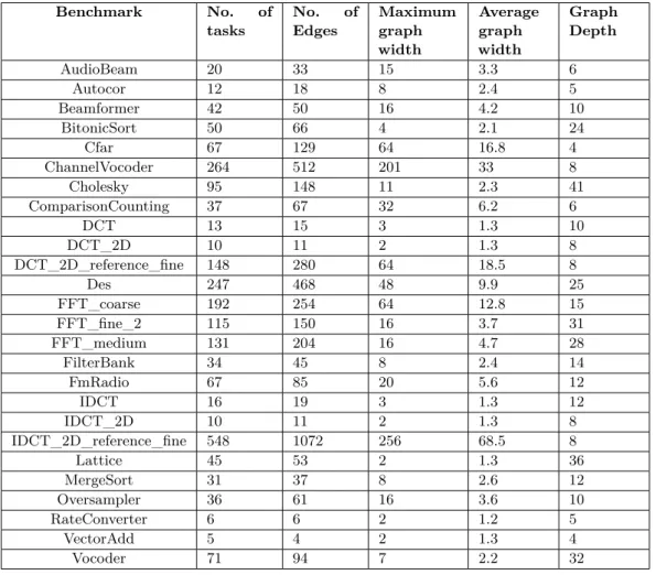
The characteristics of the obtained task graphs are summarized in Table 2. In the table, the maximum width of a task graph is defined as the maximum number of tasks with the same rank2. The maximum width defines the maximum parallelism in the benchmark. The average width is an average of the number of tasks for all ranks. The average width defines the average parallelism of the application. The higher the average width, the better the potential to benefit from a high number of cores. The depth of a task graph is defined as the longest path from the entry task to the exit task.
Additional information on the benchmarks is reported in Table 3. Reported information is the code size for the entire application, the average and standard deviation of code size per task, and the average amount of data communicated between tasks.
5.1.2
Hardware and WCET estimation
Our target architecture is the Kalray MPPA-256 machine [8], more precisely its first generation, named Andey. The Kalray MPPA-256 is a many-core platform with 256 compute cores organized in 16 compute clusters of 16 cores each. Each compute cluster has 2MB of shared memory. Each compute core is equipped with an instruction cache and a data cache of 8KB each, both set-associative with a Least Recently Used (LRU) replacement policy. An access to the shared memory, in case no contention occurs takes 9 cycles with 8 bytes fetched on each consecutive cycle [3].
Many techniques exist for WCET estimation [34] and could be used in our study to estimate WCETs and gains resulting from cache reuse. Since WCET estimation is not at the core of our scheduling methods, WCET values were obtained using measurements on the platform. Measurements were performed on one compute cluster, with no activity on the
2 The rank of a task is defined as the longest path in term of the number of nodes to reach that task
Table 2Summary of the characteristics of StreamIt benchmarks in our case studies. Benchmark No. of tasks No. of Edges Maximum graph width Average graph width Graph Depth AudioBeam 20 33 15 3.3 6 Autocor 12 18 8 2.4 5 Beamformer 42 50 16 4.2 10 BitonicSort 50 66 4 2.1 24 Cfar 67 129 64 16.8 4 ChannelVocoder 264 512 201 33 8 Cholesky 95 148 11 2.3 41 ComparisonCounting 37 67 32 6.2 6 DCT 13 15 3 1.3 10 DCT_2D 10 11 2 1.3 8 DCT_2D_reference_fine 148 280 64 18.5 8 Des 247 468 48 9.9 25 FFT_coarse 192 254 64 12.8 15 FFT_fine_2 115 150 16 3.7 31 FFT_medium 131 204 16 4.7 28 FilterBank 34 45 8 2.4 14 FmRadio 67 85 20 5.6 12 IDCT 16 19 3 1.3 12 IDCT_2D 10 11 2 1.3 8 IDCT_2D_reference_fine 548 1072 256 68.5 8 Lattice 45 53 2 1.3 36 MergeSort 31 37 8 2.6 12 Oversampler 36 61 16 3.6 10 RateConverter 6 6 2 1.2 5 VectorAdd 5 4 2 1.3 4 Vocoder 71 94 7 2.2 32
other cores, providing fixed inputs for each task. The execution time of a task is retrieved using the machine’s 64-bit timestamp counter counting cycles from boot time [8]. The effect of the timestamp counter on the execution time of a task turned out to be negligible. Since data caches are not coherent, they have to be flushed after each inter-core communication. We further observed that thanks to the determinism of the architecture, when running a task several times, in the same execution context, the execution time is constant (the same behavior was observed in [19]). For each task, we record its execution time when not reusing cache contents, as well as when executed after any possible other task.
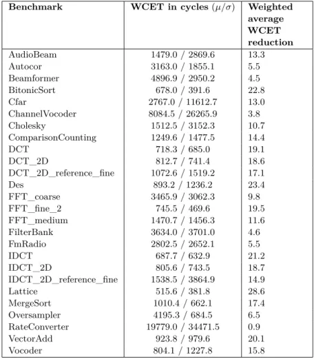
Table 4 summarizes the obtained execution times. This table shows the average and standard deviation of tasks’ WCET without cache reuse. It also shows the weighted average WCET reduction for each benchmark, computed as follows. For each task τj we calculate its
average WCET reduction in percent:
rτj = 100∗
P
τi∈nSucc(τj)
W CETτj −W CETτi→τj
W CETτj |nSucc(τj)|
(14)
Since tasks with low WCETs tend to have high WCET reductions although they have low impact on schedule length, we weighted each value by its WCET, yielding to the following
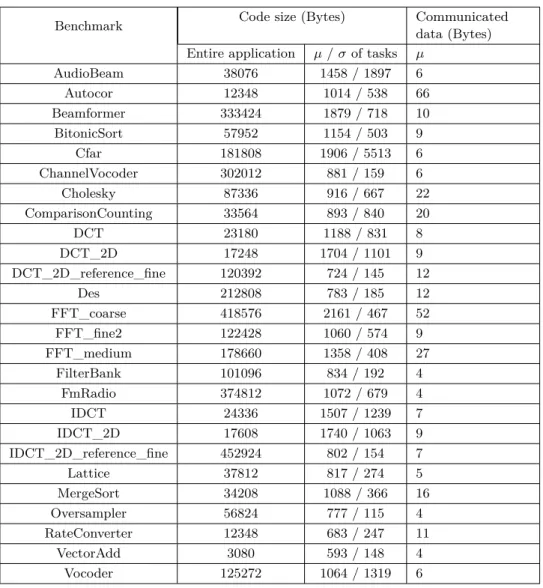
Table 3The size of code and communicated data for each benchmark (averageµand standard deviationσ).
Benchmark Code size (Bytes) Communicated
data (Bytes)
Entire application µ/σof tasks µ
AudioBeam 38076 1458 / 1897 6 Autocor 12348 1014 / 538 66 Beamformer 333424 1879 / 718 10 BitonicSort 57952 1154 / 503 9 Cfar 181808 1906 / 5513 6 ChannelVocoder 302012 881 / 159 6 Cholesky 87336 916 / 667 22 ComparisonCounting 33564 893 / 840 20 DCT 23180 1188 / 831 8 DCT_2D 17248 1704 / 1101 9 DCT_2D_reference_fine 120392 724 / 145 12 Des 212808 783 / 185 12 FFT_coarse 418576 2161 / 467 52 FFT_fine2 122428 1060 / 574 9 FFT_medium 178660 1358 / 408 27 FilterBank 101096 834 / 192 4 FmRadio 374812 1072 / 679 4 IDCT 24336 1507 / 1239 7 IDCT_2D 17608 1740 / 1063 9 IDCT_2D_reference_fine 452924 802 / 154 7 Lattice 37812 817 / 274 5 MergeSort 34208 1088 / 366 16 Oversampler 56824 777 / 115 4 RateConverter 12348 683 / 247 11 VectorAdd 3080 593 / 148 4 Vocoder 125272 1064 / 1319 6
definition of weighted average reduction:
wr= P τj∈τ(rτj ∗W CETτj) P τj∈τW CETτj (15)
5.1.3
Experimental environment
We useGurobi optimizer version 6.5 [12] for solving our proposed ILP formulation. The solving time of the solver is limited to 20 hours. The ILP solver and heuristic scheduling algorithms are executed on 3.6 GHz Intel Core i7 CPU with 16GB of RAM.
Table 4 Tasks’ WCETs (average µ / standard deviation σ) and weighted average WCET reduction.
Benchmark WCET in cycles(µ/σ) Weighted average WCET reduction AudioBeam 1479.0 / 2869.6 13.3 Autocor 3163.0 / 1855.1 5.5 Beamformer 4896.9 / 2950.2 4.5 BitonicSort 678.0 / 391.6 22.8 Cfar 2767.0 / 11612.7 13.0 ChannelVocoder 8084.5 / 26265.9 3.8 Cholesky 1512.5 / 3152.3 10.7 ComparisonCounting 1249.6 / 1477.5 14.4 DCT 718.3 / 685.0 19.1 DCT_2D 812.7 / 741.4 18.6 DCT_2D_reference_fine 1072.6 / 1519.2 17.1 Des 893.2 / 1236.2 23.4 FFT_coarse 3465.9 / 3062.3 9.8 FFT_fine_2 745.5 / 469.6 19.5 FFT_medium 1470.7 / 1456.3 11.6 FilterBank 3634.0 / 3701.0 4.6 FmRadio 2802.5 / 2652.1 5.5 IDCT 687.7 / 632.9 21.2 IDCT_2D 805.6 / 743.5 18.7 IDCT_2D_reference_fine 1538.5 / 3864.9 14.9 Lattice 515.6 / 381.8 28.6 MergeSort 1010.4 / 662.1 17.4 Oversampler 4195.3 / 684.5 6.5 RateConverter 19779.0 / 34471.5 0.9 VectorAdd 923.8 / 979.6 20.1 Vocoder 804.1 / 1227.8 15.8
5.2
Experimental results
5.2.1
Benefits of cache-conscious scheduling
In this sub-section, we show that cache-conscious scheduling, should it be implemented using an ILP formulation (CILP) or a heuristic method (CLS), yields to shorter schedules than equivalent cache-agnostic methods. This is shown by comparing how much is gained by CILP as compared to NCILP, the same ILP formulation as CILP except that cache effects are not taken into account (variablewcetτj is systematically set to the cache-agnostic WCET,
W CETτj). The gain is evaluated by the following equation, in which sl stands for the schedule length:
gain= slN CILP −slCILP
slN CILP
∗100. (16)
The gain is also evaluated using a similar formula for the heuristic method CLS (shorter schedule among CLS_BL and CLS_TL) as compared to its cache-agnostic equivalent NCLS.
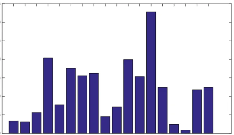
Results are reported on Figures 5 and 6 for a 16 cores architecture. In Figure 5, only the benchmarks for which the optimal solution was found in a time budget of 20 hours are depicted. These figures show that both CILP and CLS reduce the length of schedules, and
AudioBeam Autocor
BeamformerBitonic-sortCholesky DCT DCT2D FFT_fine_2FilterBankFmRadio IDCT IDCT2DLattice MergeSort
OversamplerRateConverterVectorAdd Vocoder 0 5 10 15 20 25 30 35 Gain (%)
Figure 5Gain of CILP as compared to NCILP (gain=slN CILP−slCILP slN CILP
∗100) on a 16 cores system.
this for all benchmarks. The gain is 11% on average for CILP and 9% on average for CLS. The higher reductions are obtained for the benchmarks with the higher weighted WCET reduction as defined in Table 2.
5.2.2
Comparison of optimal (CILP) and heuristic (CLS) scheduling
techniques
In this sub-section, we compare CILP and CLS according to two metrics: the quality of the generated schedules, estimated through their lengths (the shorter the better) and the time required to generate the schedules. All results are obtained on a 16 cores system.
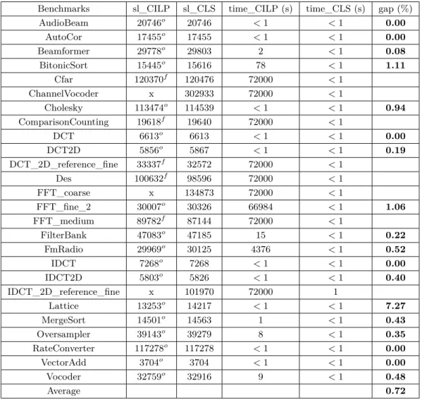
Table 5 gives the lengths of generated schedules (slCILP andslCLS), the run time of
schedule generation and the gap (in percent) between the schedule lengths, computed by the following formula:
gap= slCLS−slCILP
slCILP
∗100. (17)
The shorter the gap, the closer CLS is from CILP. The gap between CLS and CILP is given only when CILP finds the optimal solution in a time budget of 20 hours.
The table shows that CLS offers a good trade-off between the efficiency and the quality of its generated schedules. CLS generates schedules very fast as compared to CILP (i.e., about 1 second for the biggest task graphIDCT_2D_reference_finewhich contains 548 tasks). When scheduling big task graphs, such asDES,ChannelVocoder andIDCT_2D_reference_fine, CILP is unable to find the optimal solution in 20 hours. When CILP finds the optimal solution, the gap between CILP and CLS is very small (0.7% on average).
The highest gap (7.3%) is observed for theLattice benchmark. The reason is thatLattice contains a reuse pattern (illustrated in Figure 7) where reuse is higher between indirect predecessors than between direct predecessors. For example, the reduction of the WCET of T6 when executing directly after T1 (37.3%) is higher than when executing directly after
AudioBeam Autocor BeamformerBitonic-sort Cfar ChannelVocoder Cholesky ComparisonCounting DCT DCT2D DCT_2D_reference_fine Des FFT_coarseFFT_fine_2 FFT_medium FilterBankFmRadio IDCT IDCT2D IDCT_2D_reference_fine Lattice MergeSort OversamplerRateConverterVectorAdd
Vocoder 0 5 10 15 20 25 30 Gain (%)
Figure 6 Gain of CLS as compared to NCLS (gain = slN CLS−slCLS slN CLS
∗100) on a 16 cores
system.
T5 (22.6%). Similarly, the reduction of the WCET of T9 when executing directly after T4 (50.1%) is higher than when executing directly after T7 (31.3%). For such an application, the static sorting of CLS never places indirect precedence-related tasks (for which the higher reuse occurs) contiguously in the list, and then does not fully exploit the cache reuse present in the application.
5.2.3
Impact of the number of cores on the gain of CLS against NCLS
In this section, we evaluate the gain in term of schedule length of CLS against its cache-agnostic equivalent when varying the number of cores. The results are depicted in Figure 8 for a number of cores from 2 to 64.
In the figure, we can observe that whatever the number of cores, CLS always outperforms NCLS, meaning that our proposed method is always able to take advantage of the WCET reduction due to cache reuse to reduce the schedule length. Another observation is that the gain decreases when the number of cores increases, up to a given number of cores. This behavior is explained by the fact that when increasing the number of cores, the tasks are spread among cores which provides less opportunity to exploit cache reuse since exploiting the parallelism of the application is more profitable. However, even in that situation, the reduction of the schedule length achieved by CLS against NCLS is most of the time significant.
5.2.4
Impact of the number of cores on schedule length
In this section, we study the impact of the number of cores on schedule length for the CLS scheduling technique. This is expressed by depicting the ratio of the schedule length on one
Table 5Comparison of CILP and CLS (schedule length and run time of schedule generation).
Benchmarks sl_CILP sl_CLS time_CILP (s) time_CLS (s) gap (%)
AudioBeam 20746o 20746 <1 <1 0.00 AutoCor 17455o 17455 <1 <1 0.00 Beamformer 29778o 29803 2 <1 0.08 BitonicSort 15445o 15616 78 <1 1.11 Cfar 120370f 120476 72000 <1 ChannelVocoder x 302933 72000 <1 Cholesky 113474o 114539 <1 <1 0.94 ComparisonCounting 19618f 19640 72000 <1 DCT 6613o 6613 <1 <1 0.00 DCT2D 5856o 5867 <1 <1 0.19 DCT_2D_reference_fine 33337f 32572 72000 <1 Des 100632f 98596 72000 <1 FFT_coarse x 134873 72000 <1 FFT_fine_2 30007o 30326 66984 <1 1.06 FFT_medium 89782f 87144 72000 <1 FilterBank 47083o 47185 15 <1 0.22 FmRadio 29969o 30125 4376 <1 0.52 IDCT 7268o 7268 <1 <1 0.00 IDCT2D 5803o 5826 <1 <1 0.40 IDCT_2D_reference_fine x 101970 72000 1 Lattice 13253o 14217 <1 <1 7.27 MergeSort 14501o 14563 1 <1 0.43 Oversampler 39143o 39279 8 <1 0.35 RateConverter 117278o 117278 <1 <1 0.00 VectorAdd 3704o 3704 <1 <1 0.00 Vocoder 32759o 32916 9 <1 0.48 Average 0.72
–) x: no solution is found in 20 hours –) f: feasible solution is found –) o: optimal solution is found
coresl1Cores to the schedule length onncoresslnCores: slRationCores=
sl1Core
slnCores
. Results are given in Figure 9 for a number of coresn= 2,4,8,16,32 and 64. The higher the ratio, the better CLS is able to exploit the multi-core architecture for a given benchmark.
The figure shows that for all benchmarks the ratio increases up to a certain number of cores and then reaches a plateau. The plateau is reached when the benchmark does not have sufficient parallelism to be exploited by the scheduling algorithm, which is correlated to the width of its task graph as presented in Table 2.
It can be noticed that for some benchmarks (ChannelVocoder,DCT_2D_reference_fine, FFT_coarse and IDCT_2D_reference_fine) the plateau is never reached because these benchmark have too much parallelism for the number of cores. Even if the average width is below 64, we observe for these benchmarks that the maximal width is above 64 and up to 256 forIDCT_2D_reference_finewhich explains why the plateau is not reached for these benchmarks.
T1 T2 T3 T4 T5 T6 T8 T9 T7 T 10 wcetT6−wcetT1→T6 wcetT6 *100=37.3 wcetT9−wcetT4→T9 wcetT9 *100=50.1 wcetT6−wcetT5→T6 wcetT6 *100=22.6 wcetT9−wcetT7→T9 wcetT9 *100=31.3
Figure 7The reuse pattern found in theLattice benchmark.
An exception is observed forRateConverter where there is absolutely no improvement. The graph of this benchmark is an almost linear chain of tasks with only a pair of tasks that may execute in parallel. However, there is cache reuse between these two tasks and thus the best schedule, whatever the number of available cores, is obtained when assigning all tasks to the same core.
Finally, for most benchmarks, the ratio does not increase linearly with a slope of 1, because task graphs contain precedence relations.
5.2.5
Comparison of schedule lengths for CLS_TL and CLS_BL
In this sub-section, we study the impact of the sorting technique of the list scheduling technique on the quality of schedules. For each benchmark, Figure 10 depicts the ratio of the length of the schedules generated by CLS_TL to that of CLS_BL asslRatioCLS_T L/CLS_BL=
slCLS_T L
slCLS_BL
. A ratio of 1 indicates that the two techniques generate schedules with identical length. Results are given for different numbers of cores (4, 8, 16, 32 and 64).
The figure shows that there is no method which dominates the other for all benchmarks. Furthermore, the lengths of schedules generated by CLS_TL and CLS_BL are most of the time very close to each other.
There is a significant difference between CLS_TL and CLS_BL only in two cases, ChannelVocoder on 4 cores and FmRadio on 8 cores. The distances between the lengths of the schedules generated by CLS_TL and CLS_BL in these cases are then 3% and 8% respectively. It shows that in some special cases, the change in the order of tasks in the list significantly affects the mapping of tasks, hence the quality of generated schedules. Since both CS_TL and CLS_BL generate schedules very fast, we have throughout this paper always used both and selected the best result obtained.
5.2.6
Cost of estimating cache reuse
The information given in Table 6 allows to evaluate the cost of estimating cache reuse (estimation of values of W CETτi→τj) for the StreamIt benchmarks. The table reports for each benchmark its number of tasks, the number of task pairs that may be executed one after
AudioBeam Autocor BeamformerBitonic-sort Cfar ChannelVocoder Cholesky ComparisonCounting DCT DCT2D DCT_2D_reference_fine Des FFT_coarseFFT_fine_2 FFT_medium FilterBankFmRadio IDCT IDCT2D IDCT_2D_reference_fine Lattice MergeSort Oversampler RateConverter VectorAddVocoder 0 5 10 15 20 25 30 Gain(%) Scheduling on 2 cores Scheduling on 4 cores Scheduling on 8 cores Scheduling on 16 cores Scheduling on 32 cores Scheduling on 64 cores
Figure 8Impact of the number of cores on the gain of CLS against NCLS.
AudioBeam Autocor BeamformerBitonic-sort Cfar ChannelVocoder Cholesky ComparisonCounting DCT DCT2D DCT_2D_reference_fine Des FFT_coarseFFT_fine_2 FFT_medium FilterBankFmRadio IDCT IDCT2D IDCT_2D_reference_fine Lattice MergeSort Oversampler RateConverter VectorAddVocoder 1 2 3 4 5 6 7 8 slRatio nCores Scheduling on 2 cores Scheduling on 4 cores Scheduling on 8 cores Scheduling on 16 cores Scheduling on 32 cores Scheduling on 64 cores
AudioBeam Autocor BeamformerBitonic-sort Cfar ChannelVocoder Cholesky ComparisonCounting DCT DCT2D DCT_2D_reference_fine Des
FFT_coarseFFT_fine_2FFT_mediumFilterBankFmRadio IDCT
IDCT2D
IDCT_2D_reference_fine Lattice MergeSort
OversamplerRateConverterVectorAdd Vocoder 0.96 0.98 1 1.02 1.04 1.06 1.08 slRatio CLS_TL/CLS_BL Scheduling on 4 cores Scheduling on 8 cores Scheduling on 16 cores Scheduling on 32 cores Scheduling on 64 cores
Figure 10Comparison of schedule lengths for CLS_TL and CLS_BL.
Table 6Cost of estimating cache reuse.
Benchmark No. of tasks No. of possible pairs Profiling time (s)
AudioBeam 20 295 5 AutoCor 12 94 5 Beamformer 42 1326 7 BitonicSort 50 1341 7 Cfar 67 4227 11 ChannelVocoder 264 57481 170 Cholesky 95 7108 18 ComparisonCounting 37 1162 7 DCT 13 83 5 DCT_2D 10 47 5 DCT_2D_reference_fine 148 15414 49 Des 247 38185 135 FFT_coarse 192 34428 97 FFT_fine_2 115 7799 23 FFT_medium 131 10043 37 FilterBank 34 774 6 FmRadio 67 3841 11 IDCT 16 126 5 IDCT_2D 10 47 5 IDCT_2D_reference_fine 548 219238 625 Lattice 45 999 7 MergeSort 31 688 6 Oversampler 36 785 6 RateConverter 6 16 5 VectorAdd 5 11 5 Vocoder 71 2961 11
the other due to precedence constraints, and the time taken to evaluate all WCET values using measurements. The number of task pairs to be considered depends on the structure of the task graph. The worse observed profiling time is 10 minutes for the most complex benchmark structureIDCT_2D_reference_fine.
6
Conclusion
In this paper, we proposed two cache-aware scheduling techniques for applications modeled as task graphs, that generate static time-driven partitioned non-preemptive schedules for multi-core platforms. We proposed an ILP formulation as well as a heuristic scheduling method. Experimental results show that by taking into account the effect of private caches on tasks’ WCETs our proposed scheduling methods produce better schedules (in term of schedule length reduction) than their cache-agnostic equivalent. The proposed heuristic scheduling method shows a good trade-off between efficiency and the quality of generated schedules. In the future, a direct extension would be to test if exploiting reuse between more than two consecutive tasks is worth the extra complexity. We will also extend our work to deal with contentions on shared hardware resources.
Acknowledgments. The authors would like to thank Dumitru Potop-Butucaru, Benjamin Rouxel, and Biswabandan Panda for comments on earlier versions of this paper.
References
1 S. Altmeyer, R. I. Davis, L. Indrusiak, C. Maiza, V. Nelis, and J. Reineke. A generic and compositional framework for multicore response time analysis. InInternational Conference on Real Time and Networks Systems, RTNS ’15, pages 129–138, 2015.
2 J. H. Bahn, J. Yang, and N. Bagherzadeh. Parallel FFT algorithms on network-on-chips. In Fifth International Conference on Information Technology: New Generations (ITNG 2008), pages 1087–1093, 2008.
3 M. Becker, D. Dasari, B. Nikolic, B. Akesson, V. Nélis, and T. Nolte. Contention-free execution of automotive applications on a clustered many-core platform. In28th Euromicro Conference on Real-Time Systems, ECRTS, pages 14–24, 2016.
4 J. M. Calandrino and J. H. Anderson. On the design and implementation of a cache-aware multicore real-time scheduler. In21st Euromicro Conference on Real-Time Systems, pages 194–204, 2009.
5 T. Carle, M. Djemal, D. Potop-Butucaru, R. de Simone, and Z. Zhang. Static mapping of real-time applications onto massively parallel processor arrays. InProceedings of the 2014 14th International Conference on Application of Concurrency to System Design, ACSD ’14,
pages 112–121, 2014.
6 S. Chattopadhyay, A. Roychoudhury, and T. Mitra. Modeling shared cache and bus in multi-cores for timing analysis. In Proceedings of the 13th International Workshop on Software & Compilers for Embedded Systems, SCOPES ’10, pages 6:1–6:10, 2010.
7 R. I. Davis and A. Burns. A survey of hard real-time scheduling for multiprocessor systems. ACM Computing Surveys, 43(4):35:1–35:44, 2011.
8 B. D. de Dinechin, D. van Amstel, M. Poulhiès, and G. Lager. Time-critical computing on a single-chip massively parallel processor. InProceedings of the Conference on Design, Automation & Test in Europe, DATE ’14, pages 97:1–97:6, 2014.
9 H. Ding, Y. Liang, and T. Mitra. Shared cache aware task mapping for WCRT minimization. In8th Asia and South Pacific Design Automation Conference, ASP-DAC, pages 735–740, 2013.
10 G. Fernandez, J. Abella, E. Quiñones, C. Rochange, T. Vardanega, and F. J. Cazorla. Contention in multicore hardware shared resources: Understanding of the state of the art. In14th International Workshop on Worst-Case Execution Time Analysis, OpenAccess Series in Informatics (OASIcs), pages 31–42, 2014.
11 N. Guan, M. Stigge, W. Yi, and G. Yu. Cache-aware scheduling and analysis for multicores. InProceedings of the Seventh ACM International Conference on Embedded Software, EM-SOFT ’09, pages 245–254, 2009.
12 Inc. Gurobi Optimization. Gurobi optimizer reference manual, 2015.
13 D. Hardy, T. Piquet, and I. Puaut. Using bypass to tighten WCET estimates for multi-core processors with shared instruction caches. InProceedings of the 30th IEEE Real-Time Systems Symposium, RTSS, pages 68–77, 2009.
14 H. Kasahara and S. Narita. Practical multiprocessor scheduling algorithms for efficient parallel processing. IEEE Trans. Comput., 33(11):1023–1029, 1984.
15 T. Kelter, H. Falk, P. Marwedel, S. Chattopadhyay, and A. Roychoudhury. Static analysis of multi-core tdma resource arbitration delays. Real-Time Syst., 50(2):185–229, 2014. 16 Y.-K. Kwok and I. Ahmad. Benchmarking and comparison of the task graph scheduling
algorithms. InJournal of Parallel and Distributed Computing, volume 59, pages 381–422, 1999.
17 Y.-K. Kwok and I. Ahmad. Static scheduling algorithms for allocating directed task graphs to multiprocessors. ACM Computing Surveys, 31(4):406–471, 1999.
18 Y. Liang, H. Ding, T. Mitra, A. Roychoudhury, Y. Li, and V. Suhendra. Timing analysis of concurrent programs running on shared cache multi-cores. Real-time Systems, 48(6):638– 680, 2012.
19 V. Nélis, P. M. Yomsi, and L. M. Pinho. The variability of application execution times on a multi-core platform. In16th International Workshop on Worst-Case Execution Time Analysis (WCET 2016), OpenAccess Series in Informatics (OASIcs), pages 1–11, 2016. 20 V. Nélis, P. M. Yomsi, L. M. Pinho, J. C. Fonseca, M. Bertogna, E. Quiñones, R. Vargas,
and A. Marongiu. The challenge of time-predictability in modern many-core architectures. In 14th International Workshop on Worst-Case Execution Time Analysis, volume 39 of OpenAccess Series in Informatics (OASIcs), pages 63–72, 2014.
21 F. Nemer, H. Cassé, P. Sainrat, and A. Awada. Improving the worst-case execution time accuracy by inter-task instruction cache analysis. InIEEE Second International Symposium on Industrial Embedded Systems, SIES, pages 25–32, 2007.
22 R. Pellizzoni, E. Betti, S. Bak, G. Yao, J. Criswell, M. Caccamo, and R. Kegley. A predictable execution model for cots-based embedded systems. In Proceedings of the 2011 17th IEEE Real-Time and Embedded Technology and Applications Symposium, RTAS ’11, pages 269–279, 2011.
23 Q. Perret, P. Maurère, E. Noulard, C. Pagetti, P. Sainrat, and B. Triquet. Mapping hard real-time applications on many-core processors. InProceedings of the 24th International Conference on Real-Time Networks and Systems, RTNS ’16, pages 235–244. ACM, 2016. 24 Q. Perret, P. Maurère, E. Noulard, C. Pagetti, P. Sainrat, and B. Triquet. Temporal
isolation of hard real-time applications on many-core processors. In2016 IEEE Real-Time and Embedded Technology and Applications Symposium (RTAS), pages 37–47, 2016. 25 G. Phavorin, P. Richard, J. Goossens, T. Chapeaux, and C. Maiza. Scheduling with
pree-mption delays: Anomalies and issues. InProceedings of the 23rd International Conference on Real Time and Networks Systems, RTNS ’15, pages 109–118, 2015.
26 D. Potop-Butucaru and I. Puaut. Integrated worst-case execution time estimation of mul-ticore applications. In13th International Workshop on Worst-Case Execution Time Ana-lysis, volume 30, pages 21–31, 2013.
27 W. Puffitsch, E. Noulard, and C. Pagetti. Off-line mapping of multi-rate dependent task sets to many-core platforms. Real-Time Systems, 51(5):526–565, 2015.
28 H. Rihani, M. Moy, C. Maiza, R. I. Davis, and S. Altmeyer. Response time analysis of synchronous data flow programs on a many-core processor. In Proceedings of the 24th International Conference on Real-Time Networks and Systems, RTNS ’16, pages 67–76, 2016.
29 V. Suhendra, C. Raghavan, and T. Mitra. Integrated scratchpad memory optimization and task scheduling for mpsoc architectures. In International Conference on Compilers, Architecture and Synthesis for Embedded Systems, CASES ’06, pages 401–410, 2006. 30 P. Tendulkar, P. Poplavko, I. Galanommatis, and O. Maler. Many-core scheduling of data
parallel applications using SMT solvers. In17th Euromicro Conference on Digital System Design, DSD, pages 615–622, 2014.
31 C. Tessler and N. Fisher. BUNDLE: real-time multi-threaded scheduling to reduce cache contention. InIEEE Real-Time Systems Symposium, RTSS, pages 279–290, 2016.
32 W. Thies and S. Amarasinghe. An empirical characterization of stream programs and its implications for language and compiler design. In Proceedings of the 19th International Conference on Parallel Architectures and Compilation Techniques, PACT ’10, pages 365– 376, 2010.
33 B. C. Ward, A. Thekkilakattil, and J. H. Anderson. Optimizing preemption-overhead accounting in multiprocessor real-time systems. InProceedings of the 22Nd International Conference on Real-Time Networks and Systems, RTNS ’14, pages 235:235–235:243, 2014. 34 R. Wilhelm, J. Engblom, A. Ermedahl, N. Holsti, S. Thesing, D. Whalley, G. Bernat,
C. Ferdinand, R. Heckmann, T. Mitra, F. Mueller, I. Puaut, P. Puschner, J. Staschulat, and P. Stenström. The worst-case execution-time problem: Overview of methods and survey of tools. ACM Trans. Embed. Comput. Syst., 7(3):36:1–36:53, 2008.
35 G. Yao, R. Pellizzoni, S. Bak, E. Betti, and M. Caccamo. Memory-centric scheduling for multicore hard real-time systems. Real-Time Systems, 48(6):681–715, 2012.
![Figure 1 Task graph of a parallel version of a 8-input Fast Fourier Transform (FFT) application [2].](https://thumb-us.123doks.com/thumbv2/123dok_us/10114412.2911993/2.892.321.599.151.440/figure-task-graph-parallel-version-fourier-transform-application.webp)