Theoretically Consistent Temporal Ordering Specification in Spatial Hedonic Pricing Models Applied to the Valuation of Aircraft Noise
Sotirios Thanos^, Abigail L. Bristow*, Mark R. Wardman**
Abstract
Incorporating spatial econometric tools in Hedonic Pricing (HP) models for environmental valuation has become the standard approach in the literature. The effect of house prices on other house prices is taken into account and usually measured by distance or contiguity in spatial weight matrices. Disaggregate house sale datasets are composed from observations each at a specific location and time. Nevertheless, the symmetric spatial weight matrices commonly employed in HP studies ignore the temporal dimension in disaggregate house sale data. Thus not only are previous house sales taken to affect subsequent house prices, but so do future house sales. However, information does not travel backwards in time; hence there is a clear theoretical impossibility of actual future prices affecting current/past prices. Estimates derived from HP models where spatial dependence is incorrectly specified or ignored will exhibit inaccuracies. This paper proposes an alternative specification of spatial weights in HP that includes spatial effects on each sale price only from preceding house sales. The temporal aspect of spatial effects is then developed further by specifying a time decay rate to capture the diminishing effect over time of preceding sale prices to succeeding house prices. This novel specification of spatial weight matrices is shown to have a significant effect on estimates of house price depreciation from aircraft noise. Monetary values of aircraft noise externality are successfully derived from the HP models for Athens Airport.
Keywords: Spatial Econometrics, Spatial Autocorrelation, Aircraft Noise, Environmental Valuation, Hedonic Pricing, Time Decay
JEL classifications: C21, Q51, Q53, R41
^Corresponding Author, School of Built Environment, Heriot-Watt University, EH14 4AS, Edinburgh, UK, Email : [email protected], Tel : +44 (0)131 451 4641
* School of Civil and Building Engineering, Loughborough University ** Institute for Transport Studies, University of Leeds
1. Introduction
Noise disturbance is a serious environmental issue and a key externality of the aviation sector, raising health, economic and social concerns (Berglund et al., 1999; Miedema, 2007). Around 6.9 million people in Europe are exposed to aviation noise levels exceeding 55dBA and the numbers are expected to grow in the absence of further policy intervention (European Environment Agency, 2010). Valuation of the costs of aircraft noise annoyance can inform policy and appraisal. Hedonic Pricing (HP) techniques are traditionally relied upon to identify the impact of aviation noise on house prices (Nelson, 2008).
HP posits that the price of a composite commodity, such as housing, is a function of its characteristics, including the level of quietness (absence of noise). The quantity of hedonic studies on aircraft noise is such that a number of meta-analyses have been carried out. The most recent by Wadud (2010) included 53 estimates of house price depreciation from aircraft noise and concluded that a 1 dBA change in aircraft noise levels leads to house price depreciation between 0.45% and 0.64%. This estimate is broadly consistent with earlier analysis by Nelson (2004) and the early review by Nelson (1980) though somewhat lower than the estimates of Schipper et al. (1998) of 0.9% to 1.3%. Whilst aircraft noise exposure is a negative externality, distance to the airport is often found to positively affect house prices (Tomkins et al., 1998), underlining the importance of the spatial dimension in such analysis. The notion of spatial dependence stems from the first law of geography stating that “everything is related to everything else, but near things are more related than distant things” (Tobler 1970, pp. 236). During the past decade spatial econometrics has moved to the mainstream of applied econometrics and social science methodology (Anselin, 2010). Consequently, the scope of spatial econometrics has been further developed and broadened from the cross-sectional to the space-time domain (Anselin, 2006). Spatial econometrics is defined as “a subset of econometric methods that is concerned with spatial aspects present in cross-sectional and space-time observations. Variables related to location, distance and topology are treated explicitly in model specification; estimation; diagnostic checking and prediction” (Anselin, 2006, pp. 902). We are interested here in the case of spatial dependence that typically takes the form of weighted averages of observations for the ‘neighbours’ of a
given location (Anselin, 2010). Spatially lagged variables are included to capture these effects, specified by a spatial weights matrix.
A number of studies have now combined spatial econometrics and HP models to value environmental attributes and transportation noise; examples include Conway et al. (2010), Andersson et al. (2010), Day et al. (2007), Hui et al. (2007) and Kim et al. (2003). A few studies have also combined spatial econometrics and HP models to produce aircraft noise valuation estimates (Bateman et al., 2004; Salvi, 2008; Cohen and Coughlin, 2008; Dekkers and Van der Straaten, 2009; Chalermpong, 2010), whilst Theebe (2004) combined rail, road and aircraft noise into a single noise index. Not all of these studies produce statistically significant HP estimates for aircraft noise and there are also some shortcomings in the treatment of aircraft noise in the HP modelling regarding the quality of the noise data and the treatment of background noise that are examined in detail in section 5.
Anselin (2002, pp. 259) stresses that “there is very little formal guidance in the choice of the ‘correct’ spatial weights in any given application”. This does not mean that there are no cases where the spatial weight specification is plainly incorrect. Most HP models are based on analysis of disaggregate house sale data, composed from observations each at a specific location and time. Spatial distance or contiguity is normally the only factor taken into account when specifying spatial weights for such data. However, there is an element of temporal ordering in disaggregate house sales datasets that ought to be taken into account. Ignoring the arrow of time produces paradoxical assumptions, such as a house sale price being affected by house sales that have not taken place yet. Henceforth, this is termed the “temporal ordering inconsistency”, where interdependence of house prices is assumed instead of the correct uni-directional effect from earlier to subsequent house sales only. Even though expectations and speculation for future prices or forecasting may well affect current prices, all these strictly depend on information from the past and the present. Information does not travel backwards in time; hence there is a clear theoretical impossibility of actual future prices affecting current prices.
Temporal ordering has been recognised and accounted for in the real estate literature, as part of modelling the spatiotemporal patterns of house prices to produce robust house price indices. To that effect spatiotemporal models on panel data have been employed, often using HP model results as inputs (Pace et al., 1998; Gelfand et al., 2004). Can and Megbolugbe
(1997), accounting for spatial dependence in house price index construction, allow only prior sales to influence house prices in their HP models, directly addressing the temporal ordering inconsistency. In section 4 we discuss their approach and its shortcomings, improving the methodology and applying it to environmental externality valuation.
The HP literature valuing environmental commodities does not appear to recognise the temporal ordering issue. Judging from the information provided about the nature of the data and the specification of spatial weights in the published papers, some of the aircraft noise HP studies (Chalermpong, 2010; Dekkers and Van der Straaten, 2009; Salvi, 2008; Theebe, 2004) and some looking at other environmental characteristics (Conway et al., 2010; Andersson et al., 2010; Hui et al., 2007) suffer from temporal ordering inconsistencies. Others, for example, Cohen and Coughlin (2008) and Bateman et al. (2004) attempt to avoid this issue by assuming that the house sale observations cover a single time period (i.e. a year) so no temporal ordering is imposed in their data. Kim et al. (2003) avoid the temporal ordering inconsistency, as their models are not based on house sales, but on survey data and respondents’ estimates of their current house value. The spatial interaction is between geographical areas, where interrelationship is a reasonable assumption (Franzese, and Hays 2008).
The key contribution of this paper is to propose an elegant solution to the temporal ordering inconsistency and to demonstrate that the treatment of this inconsistency affects the estimation of aircraft noise depreciation. We also go a step further forward to specify a time decay rate capturing the over time diminishing effect of preceding sale prices to succeeding house prices. Additionally, the specification of aircraft noise in our models employs continuous noise data, explicitly including an allowance for background noise and avoiding the imposition of artificial thresholds (Thanos et al., 2011; Andersson et al., 2010), which we believe is an advance on previous practice in HP studies valuing aircraft noise.
The structure of this paper is as follows. Section 2 briefly discusses the theoretical background of the HP method. Section 3 describes the housing data and the derived geographical information. Section 4 explains spatial dependence, the approaches in the literature and our approach. Section 5 illustrates the shortcomings of aircraft noise treatment in the recent spatial HP literature and discusses our approach to aircraft noise modelling.
Section 6 presents the HP modelling methodology and discusses the HP results. The conclusions follow in Section 7.
2. Hedonic Pricing
Rosen’s (1974) two stage hedonic pricing approach was an important theoretical contribution that has become the cornerstone of most empirical work on housing markets. In the first stage, using data on house prices and characteristics, the hedonic price schedule is estimated, from which implicit marginal prices for housing characteristics are calculated (Nelson, 2008). However, implicit prices are market specific, reflecting only the particular situation of supply and demand that exist in a given property market and offering little indication of the conditions and marginal prices in other housing markets (Day et al., 2007). The second stage involves the marginal prices of a characteristic, combined with data on occupants’ income and other socioeconomic variables, to estimate an inverse demand function (Nelson, 2008). This is a theoretically and analytically challenging task whilst the problem is in essence quite simple. Information is required on at least two points along the length of a household’s demand curve, whereas data from a single housing market provide just one such point (Day et al., 2007).
Only Day et al. (2007) have applied the second stage HP approach in noise valuation and estimated an inverse demand function for road traffic and rail noise. All other noise valuation studies, including our approach, are estimating the first stage hedonic pricing schedule, reporting marginal prices of housing characteristics. The first stage hedonic price function (P) of a composite commodity, housing in this case, may be written as:
P = P (γ, Z) (1)
where Z = [z1, . . . , zm] is a vector of utility bearing characteristics and γ is aircraft noise exposure. The slope of the HP price function can be used to determine the consumer’s marginal willingness to pay for a given commodity (characteristic), since in optimum it equals her marginal rate of substitution between the price of the commodity and any of the other housing characteristics (Rosen, 1974; Andersson et al., 2010). This marginal WTP for aircraft noise is:
,
(2)
Eq. 2 only shows the marginal WTP in optimum, obtained by the information of individuals’ behaviour at a point in time; it does not reveal the underlying preference structure (Andersson et al., 2010). Moreover, welfare measurements are not possible using only marginal prices, unless the environmental change affects a small number of houses relative to the size of the market (Palmquist, 1992). This special case of a localised externality is applicable to our research context as we only examine a small part of the housing market of metropolitan Athens.
3. Housing Data
This study employs data on 1613 house sales from 1995 to the beginning of 2001, acquired by local real estate consultants1 around Athens International Airport (AIA). Aircraft noise had been a very important issue in this densely populated area (Charalampakis, 1980), which had more than 350,000 residents in 2001 (National Statistical Service of Greece, 2003). The data include information about the basic structural characteristics of each house, such as the square meters of the floor for the living space2, construction year, sale date, number of rooms3, presence of a garage and floor number. The house type is categorised as detached, semidetached/terraced and flat. The sale price of each house is given in €s converted from drachmas. A quarterly consumer price index for the housing sector in Greece (OECD, 2006) was used to adjust the prices to 2001 levels.
The full address of each house sale was available, allowing the assignment of geographical coordinates to each house (with 20 meters accuracy or better) and the derivation of further geographical information through GIS modelling. Certain local amenities have been shown to affect house prices (Frankel, 1988; Bateman et al., 2001). We located 445 such amenities in the area and used the specific coordinates to estimate the crow fly distance between each house and the nearest church, public service facility, sport facility, hospital or health centre,
1 “Property AE”, was an established real estate consulting firm at the time, specialised in housing market studies
and connected with local real estate agents and the National Bank of Greece, published the “real estate news” magazine.
2 Excluding balconies, gardens and sheds
plaza, super market and school. The premium of a seaside location is controlled for by introducing a dummy for houses within 300 meters of the coastline4.
Digital maps5 and local road network data were acquired. The road distance from each house
igure 1 illustrates all the available geographical information for the study area, including the
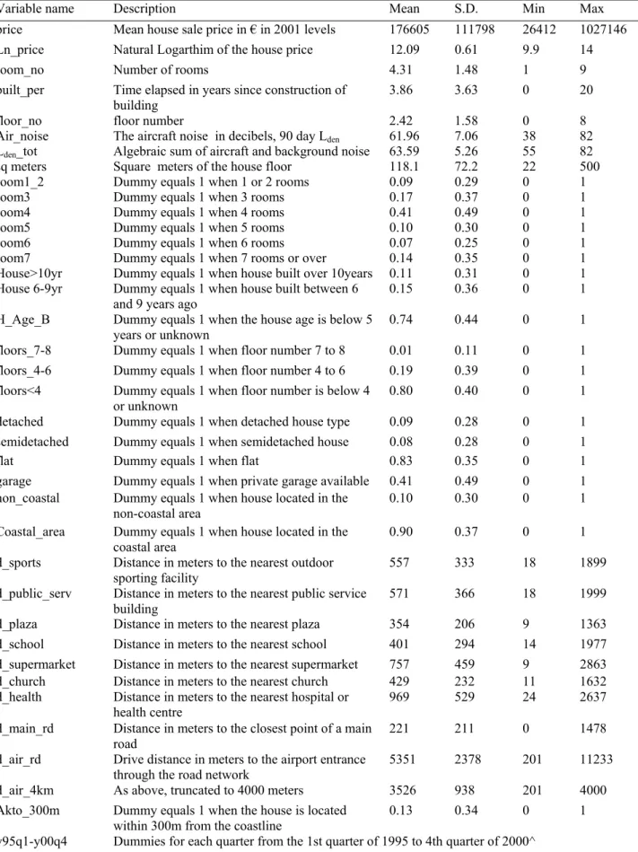
able 1 provides the details of all available data. Most of the data refer to newly constructed
ooking at the spatial distribution in figure 1 the data provide good coverage for all the areas
to the Airport entrance was then estimated, since access to the airport is usually by car or public transport rather than on foot, as would be the case for many other local amenities in close proximity. These data also allowed the estimation of the distance to the closest point of a main road for each house. This is expected to account for better accessibility, but also for additional road noise, for which we do not have any other available information.
F
location of each house sale, the road network, the main roads, the airport entrance, the coast line and the amenities in the area.
T
properties; 73% were built within 5 years of the sale and 83% are flats. This is due to the high development rate of the local housing market during the study period. The market was in the process of replacing older, lower quality and low rise houses (detached/semidetached) with high rise flat complexes. We are confident that our data sample reflects the situation in the local housing market during the study period. This was also supported by the interviews conducted with local real estate agents and housing market professionals in 2004. We were unable to confirm this from official data sources in Greece, since appropriate data were simply not available for the area and study period.
L
(the road network indicates the inhabited part of the map), with coastal areas having the highest observation density. The estimation of aircraft noise exposure data is discussed in section 5.
4 We did not use a continuous distance to the coast variable, because it did not capture the amenity of residing
near the sea for observations further inland. Instead the inclusion of this variable introduced collinearity in the models. We tested a range of dummy variables and the 300 meter dummy provided best statistical fit.
Figure 1: The geographical features of the study area and the location of each house sale
Table 1: Data description
Variable name Description Mean S.D. Min Max
price Mean house sale price in € in 2001 levels 176605 111798 26412 1027146 Ln_price Natural Logarthim of the house price 12.09 0.61 9.9 14
room_no Number of rooms 4.31 1.48 1 9
built_per Time elapsed in years since construction of
building 3.86 3.63 0 20
floor_no floor number 2.42 1.58 0 8
Air_noise The aircraft noise in decibels, 90 day Lden 61.96 7.06 38 82
Lden_tot Algebraic sum of aircraft and background noise 63.59 5.26 55 82
sq meters Square meters of the house floor 118.1 72.2 22 500 room1_2 Dummy equals 1 when 1 or 2 rooms 0.09 0.29 0 1
room3 Dummy equals 1 when 3 rooms 0.17 0.37 0 1
room4 Dummy equals 1 when 4 rooms 0.41 0.49 0 1
room5 Dummy equals 1 when 5 rooms 0.10 0.30 0 1
room6 Dummy equals 1 when 6 rooms 0.07 0.25 0 1
room7 Dummy equals 1 when 7 rooms or over 0.14 0.35 0 1 House>10yr Dummy equals 1 when house built over 10years 0.11 0.31 0 1 House 6-9yr Dummy equals 1 when house built between 6
and 9 years ago
0.15 0.36 0 1 H_Age_B Dummy equals 1 when the house age is below 5
years or unknown 0.74 0.44 0 1
floors_7-8 Dummy equals 1 when floor number 7 to 8 0.01 0.11 0 1 floors_4-6 Dummy equals 1 when floor number 4 to 6 0.19 0.39 0 1 floors<4 Dummy equals 1 when floor number is below 4
or unknown
0.80 0.40 0 1 detached Dummy equals 1 when detached house type 0.09 0.28 0 1 semidetached Dummy equals 1 when semidetached house 0.08 0.28 0 1
flat Dummy equals 1 when flat 0.83 0.35 0 1
garage Dummy equals 1 when private garage available 0.41 0.49 0 1 non_coastal Dummy equals 1 when house located in the
non-coastal area 0.10 0.30 0 1
Coastal_area Dummy equals 1 when house located in the
coastal area 0.90 0.37 0 1
d_sports Distance in meters to the nearest outdoor
sporting facility 557 333 18 1899
d_public_serv Distance in meters to the nearest public service
building 571 366 18 1999
d_plaza Distance in meters to the nearest plaza 354 206 9 1363 d_school Distance in meters to the nearest school 401 294 14 1977 d_supermarket Distance in meters to the nearest supermarket 757 459 9 2863 d_church Distance in meters to the nearest church 429 232 11 1632 d_health Distance in meters to the nearest hospital or
health centre 969 529 24 2637
d_main_rd Distance in meters to the closest point of a main road
221 211 0 1478 d_air_rd Drive distance in meters to the airport entrance
through the road network 5351 2378 201 11233
d_air_4km As above, truncated to 4000 meters 3526 938 201 4000 Akto_300m Dummy equals 1 when the house is located
within 300m from the coastline 0.13 0.34 0 1 y95q1-y00q4 Dummies for each quarter from the 1st quarter of 1995 to 4th quarter of 2000^
4. Spatial dependence in HP and temporal ordering
ndence o ption in ono ic est ion P
s using squares (OLS) regress h the a umptio of
ndence ed spatial
ence. Th nd biase dard r estim s, aff ing
nce leve lu nsel 003; son, ),
ing OLS ing spatial enden
e housing errors are seen rise f ther o e foll ing
ns (A p of a house is not only affected
ributes se mity. In this case a spatial lag
(SLM) i a lagg rice o ervati of
uring h ent ble. e sec d cas the
ntain sy
requiring what Spatial Error Model (SEM), illustrated in Eq. 5. This is appropriate
ses sh atial rn an se am ities c not
e controlled fo , 2008).
tural f
(0, σ²I) (3)
and its reduced
ral f
(
Where educed form of SEM is given by:
, u ~ N(0, σ²I) , (6)
Where P is a vector of the house prices, X is a matrix of housing characteristics and b is a
e coefficien cture between obs
the spatial weig spatial dependence coefficients that are estimated uced to OLS models, if ζ or λ respectively re equal to zero.
Indepe f residuals is an essential assum the ec metr imat of H
model ordinary least ions. W en ss n
indepe between observations across space is violated, this is term
depend is leads to inefficient estimators a d stan erro ate ect confide ls for the coefficients and predicted va es (A in, 2 Nel 2008 render inappropriate for models contain dep ce.
In th market, spatially dependent to a or ei f th ow
two reaso nselin, 2003; Nelson, 2008). Firstly, the rice by its att but also by the prices of houses in clo proxi
model s appropriate, shown in Eq. 3, where sp tially ed p bs ons neighbo ouses are included as an independ varia In th on e, residuals co stematic spatial information that is not captured by
is termed a
the regression model, when hou are common amenities that have a sp patte d the en an b r (Anselin, 2003; Nelson
The struc orm of the SLM is: , ε ~ N
form is:
(4)
The structu orm of SEM is:
5) . The r
vector of th ts. The spatial correlation stru ht matrix W. ζ or λ are the
ervations is given by in the modelling process. SLM and SEM are red
The presence of a lagged price variable in SLM denotes that the total increase in value due to
l multiplier effect halermpong, 2010) or assume the issue away (Andersson et al., 2010). Cohen and
tion, where everything is correlated with verything else (Conway et al., 2010) but does not address temporal ordering.
Imposing contiguity
g market and urban space. One needs to specify units, within which the observations behave in the sam
limited. Submarket effects are not always distributed spatially and spatial sub-markets do not ften coincide with administrative areas (Watkins, 2001, Bateman et al., 2004). Rather than he similarity of property characteristics or geographical contiguity,
conomic characteristics of the local population (Bateman et al., 2004).
a change in an attribute can be decomposed into a direct and an indirect effect. The latter occurs when the increased value of the property in question raises the value of neighbouring properties that in turn raise the value of the property in question further (Andersson et al., 2010). Eq. 4 demonstrates that the marginal implicit price in SLM for attribute ω is not given by bω, but by bω (Kim et al., 2003), where is termed spatial
multiplier. Some HP studies that use SLM disregard the spatia (C
Coughlin (2008) estimate spatial multiplier effects for noise and discuss the indirect spatial effects. This is not an issue in SEM.
4.1. Spatial weight specification
Spatial weights are usually based on distance or contiguity. In defining contiguity weights, areas (polygons) adjacent with the targeted area (polygon) of the house sale are assigned a weight of 1 in the weighting matrix, and all other areas a weight of 0. This approach reduces the probability overestimation of spatial correla
e
weights introduces unverifiable assumptions about the structure and the interactions of the housin
e way and adjacent units to which the interactions are o
being based exclusively on t
the dimensions of housing submarkets are determined by both spatial and structural factors simultaneously (Watkins, 2001) and socioe
Therefore, we prefer distance based spatial weights for HP models. We specify the weights as the inverse distance between house sale observations following Can and Megbolugbe (1997). This accounts for the diminishing effect of house sales prices that are further from each other.
The spatial weights are in the form of a square n×n matrix W. We specify three distance based spatial weight matrices Wα, Wβ and Wγ. Each element wij in matrix Wα is given by:
i j
0 i j (7)
Where dij is simply the inverse Euclidean distance between house i and house j. Wα is a
symmetric square matrix with the main diagonal being zero (the effect of each sale price to itself). This is simil mmon approach in the literatu istance weights are employed and contains the temporal ordering inconsistency.
One important consideration in specifying spatial weight matrices is to avoid overestimation of spatial dependence, where each
ar to the co re, when d
observation is spatially connected to every other bservation and vice versa and other factors are underestimated. Most studies that employ
y cut-off point, after which house prices are not ssumed to affect each other within an urban structure. For example, Andersson et al. (2010)
ctively a case f overestimating spatial dependence, mistaking a uni-directional relationship for two way
ver, a year is too long a period to be considered as a multaneous sale for all the data (Pryce and Gibb, 2006; Zuelke, 1987; White and Watkins, 2004). Even if they do not have the information to address temporal ordering, it is still in the o
distance based weights introduce an arbitrar a
present two models with cut off points at 4km and 10km. Kim et al. (2003) consider as neighbours all housing units in the same sub-district as well as all units in districts that have their centroid within 4 km. Bateman et al. (2004) introduce much lower cut-off points of about 0.25 km for various sub-market HP models. Similarly Chalermpong (2010) and Salvi (2008) use a 0.3 km cut-off point. The temporal ordering inconsistency is effe
o
interdependence. In addressing the temporal ordering inconsistency, we account for part at least of any spatial dependence overestimation, as is discussed below.
Looking the aircraft noise spatial HP literature, Dekkers and Van der Straaten, (2009), Theebe (2004), Salvi (2008) and Chalermpong (2010) specify their spatial weight matrices in a way that includes the temporal ordering inconsistency. Cohen and Coughlin (2008) and Bateman et al. (2004) assume that the house sale observations cover a single period, a year. If no more specific information about sale dates is available, they would not be able to impose any temporal ordering in their data. Howe
data, since they employ symmetric spatial weight matrices that assume interdependence between the sale prices. Hence, there is still overestimation of spatial dependence due to temporal ordering, even if some overestimation is dampened through arbitrary cut-off points. As our case study area is a relatively small geographical part of Athens where everything
ffects everything else, albeit to a small degree, we do not specify any distance cut-off point. There is no theoretical reason but only methodological necessity/convenience. However, the inverse distance specification em
sales prices that are further from each other. To address the temporal ordering inconsistency a
ployed here accounts for any diminishing effect of house that is present in Wα, we specify matrix Wβ with each element wij given by:
i j
0 / i j (8)
Where ti and tj is the number of days elapsed since the first observation in the dataset and the
sale of houses i and j respectively. When the data are ordered from the “furthest in the past” to the latest house sale, Wβ becomes a lower triangle square matrix, with all the values of the upper triangle being zero. Only sales in the past affect subsequent sales and not vice versa. Thus Wα contains double the information of Wβ, even though this information is the product of the paradoxical assumption of sales prices being affected by sales that have not yet taken place. We expect that due to this extra information Wα will produce better fitting models than Wβ, overestimating spatial dependence. Hence, overall goodness of fit measures cannot provide guidance to choosing the preferred model in this context; only theoretical considerations can help.
One of these theoretical considerations is the assumption in Wβ that sale prices further in the past should affect a current sale price to the same extent as more recent sale prices. An
lowance for temporal distance, maybe in the form of a time decay factor, may therefore be al
an appropriate addition to the distance weights that specify the connection in space between the observations. In the current model form it is not computationally feasible to estimate a time decay function on the top of the estimated spatial parameters. The time decay factor must be specified a priori. Hence, we look at the housing economics literature for clues as to what time frame may be appropriate when considering a decay factor for the spatial weights.
Pryce and Gibb (2006) show that about 80% of the properties on sale in Strathclyde are sold within 1 quarter and about 90% of the properties are sold within 2 quarters. Zuelke (1987) find the average market duration of a house on sale in Florida being about 4 months and less than 6 months for the 82% of their sample. White and Watkins (2004) determine that the vast majority of the properties on sale in Aberdeen were sold within 95 days. We assume that rice setting behaviour of the seller is mostly affected by the price levels at the time and the
ales is reducing onlinearly with passing time. Sales far in the past can be seen as providing a background in the market. We combine these insights to specify a new weight matrix. Each matrix element of inverse Euclidean distance be
between the two sales. Thus our approach diverges from Can and Megbolugbe (1997), who referred spatial weight specification all prior sales that occurred within a p
same goes for the buyer, when he is doing market research.
The time-on-the-market studies above indicate that the time scale, in which house market participants are most exposed to effects from past house sales, is within a quarter of the sale. Hence, this may be the most appropriate time frame in which to analyse these effects. We further assume that the effect on subsequent house prices from past s
n
tween two observations is divided by the number of quarters include in their p
3km of a current transaction and only within the prior two quarters. This way they are setting cut off points in both space and time. As discussed above, we do not see any reason to set distance cut off points in this context and the effects of past sales to subsequent house prices is dampened after two quarters instead of being assumed zero.
More formally, to take account of time decay we specify the weight matrix Wγ, by multiplying each element wij in Wβ by the time decay rate rij:
i j
1 i j (9)
Where qi and qj are the quarters during which houses i and j were sold respectively, with q
This implies that the bigger difference between the quarters of any two house sales, the less the spatial weight in the modelling. For example if house j was sold 2 years before house i it loses 87.5% of the weight it would have if the sales took place in the same quarter. Houses sold in the same quarter or within a quarter of each other are weighted by the inverse distance
ure
on and thresholds.
ft noise depreciation on house rices for 1 dBA increase, which is rather on the high side of the HP literature. A reasonable
without any effect from rij. The feature of Wβ, where sale prices cannot affect the prices of
preceding house sales is kept in Wγ. Hence, negative values of rij are unimportant, since they
multiply zeros in upper triangle part of the matrix Wβ.
5. Aircraft Noise
5.1. The treatment of noise in the spatial HP literat
Here we consider the treatment of aircraft noise in the published studies that apply spatial HP models to aircraft noise valuation. Issues include the use of continuous or banded data, the use of cut-off or threshold values and the treatment of background noise.
Theebe (2004), Cohen and Coughlin (2008) and Chalermpong (2010) use a dummy variable specification for noise, producing statistically significant estimates only above 65dBA, 70dBA and 70-75dBA6 respectively, all of which are very high levels of noise exposure. Chalermpong (2010) also has a serious data constraint7, which might affect the aircraft noise estimates. Theebe (2004) transformed continuous noise data to 5 dBA noise bands. We consider dummy specifications (constructed from noise contours/bands or continuous data) as an inferior approach to continuous aircraft noise exposure data. Dummy specifications make no distinction between properties within a contour. The noise banding also imposes untestable assumptions about functional form of noise depreciati
Regarding the studies that employed a continuous aircraft noise variable, Salvi (2008) produced a statistically significant estimate of 0.97% aircra
p
es 30-35 and 35-40 Noise Exposure Forecast (NEF) contours that closely correspond to
6 Chalermpong (2010) us
65-70 and 70-75 dBA of Ldn metric respectively. Ldn is the equivalent continuous sound pressure level over a
fixed time period (Leq) where the night values (22:00 – 06:00) are weighted by the addition of 10 dBA. t is stated that most of the 37,591 observation had identical characteristics and were sold at the same price. Therefore, the dataset was restricted to only 384 observations for the HP modelling. It is not made clear how these 384 observations were selected, since 554 observations of the extended dataset were in the 35-40 NEF contour and 1784 in the 30-35 NEF contour.
threshold of 50 dBA was employed for both aircraft and road traffic noise. Bateman et al. (2004) could not attribute any statistically significant effect to aircraft noise, using a common ut off point across modes of 55dBA below which it was assumed that transport noise was
is problematic, especially the explicit assumption that below a reselected level aircraft noise does not impact on values. The inclusion of noise from other
(2009) do, is an attempt allow for background noise. However, the use of different thresholds in Dekkers and Van
dBA.
n for the afety of Air Navigation (EUROCONTROL), who have complete data on flight paths and aircraft movements for Hellenikon Airport. Radar data were employed to derive more
he of c
indistinguishable from ambient noise. Dekkers and Van der Straaten (2009) report a model with thresholds that vary by the noise source, 45 dBA for air traffic, 55 dBA for road and 60 dBA for rail, recovering a statistically significant effect for aircraft noise of 0.77% depreciation per dBA on house prices. The authors noted that threshold selection influenced their aircraft noise value estimates, with the coefficient becoming insignificant at threshold levels equal to or above 50dBA. They do not report the effects of changing the road and rail noise threshold levels.
The use of thresholds p
transport modes, as Salvi (2008) and Dekkers and Van der Straaten to
der Straaten (2009), whilst reflecting evidence in the annoyance literature is questionable in this context. They are effectively assuming that road traffic noise will not impact on welfare until it is 55dBA, whereas aircraft noise will do so at half the intensity, 45
Nonlinear econometric specifications of the noise variable may arbitrarily impose a predetermined functional form, as a concave function in Andersson et al. (2010). Such approaches also require estimation of additional parameter(s) in models that cannot simultaneously account for spatial dependence (Kim et al., 2003). Hence, such specifications are not employed in this paper.
5.2. Treatment of aircraft and background noise in this study
The physical aircraft noise estimates were supplied by the European Organisatio S
accurate aircraft approaches to the airport and the Integrated Noise Model (Federal Aviation Administration, 2003) was employed for the aircraft noise modelling. The consistency of t modelled data with actual noise measurements was confirmed by EUROCONTROL. A set
coordinates for each house sale was provided to EUROCONTROL and they supplied an estimate of the aircraft noise exposure for the specific coordinates.
The noise exposure data is in the Lden8 noise metric, which is seen as appropriate for aircraft noise in the EU (EC, 2002) and is commonly used in HP studies valuing noise (Dekkers and Van der Straaten, 2010; Rich and Nielsen, 2004; Baranzini and Ramirez, 2005). Miedema et al. (2000) investigated which noise metrics best predict annoyance from aircraft noise and supported the use of weighted noise metrics, such as Lden, instead of Leq in this context.
The decibel value provided represents the average value of the 90 day period preceding the house sale. This is to prevent the decibel value reflecting daily, weekly or monthly peaks that can be misleading for this kind of analysis. This averaged value is expected to better reflect the effect of aircraft noise exposure on housing market actors prior to house purchase.
learly we wish to take account of background noise pollution from road traffic and other The basic descriptive statistics for aircraft noise exposure are found in Table 1 under the “Air_noise” variable. Figure 2 visually illustrates this exposure on our housing data using 5 decibel contours. There is much variation in aircraft noise exposure across the study area reaching a maximum of 82 dBA. Residents in the municipality of Alimou (north-northwest of the airport) were exposed to by far the highest noise levels, as noted elsewhere in the literature (Yang and Kang, 2005; Charalampakis, 1980).
C
sources. Unfortunately, no data were available on other sources of noise pollution such as road traffic. From previous studies of the noise situation in Athens (Nicol and Wilson, 2004; Yang and Kang, 2005), it can be deduced that a 55dBA value for background noise would be a reasonable approximation. In addition we used distance to a major road as a proxy for higher exposure to traffic noise.
8 Equivalent continuous sound pressure level over a fixed time period (L
eq), where the evening values (18:00 –
22:00) are weighted by the addition of 5 dBA (A-weighted decibel), and the night values (22:00 – 06:00) are weighted by the addition of 10 dBA
We attempt to capture the effect of aircraft noise on the housing market above the general noise level in the area, even if aircraft noise effects are very low when dominated by other noise sources. Following Andersson et al. (2010) and Thanos et al. (2011), the aircraft noise level (γa) and the assumed background noise level (γb) are combined in a total noise level (γt)
that is given by:
⎟⎟
⎠
⎞
⎜⎜
⎝
⎛
+
=
10 10 1010
10
10
)
,
(
a bLOG
a b t γ γγ
γ
γ
(10)The γt is used in HP models. If γa is dominant, γb will have an almost negligible effect on the
total noise level and vice versa (γa γb ≈ γa if γa γb). This analysis can be considered a
step forward from studies that simply examine variations in aircraft noise above a pre-specified cut off point. Even low levels of aircraft noise are included in the analysis that would otherwise have been below a 55 dBA cut off point; for example 51 dBA aircraft noise and 55 dBA background produce a total noise level of 56.46 dBA.
Variable “Lden_tot” in Table 1 provides the descriptive statistics for γt. The difference
between the mean noise total (63.59 dBA) and the mean of only aircraft noise (61.96 dBA) is 1.63 dBA, indicating that aircraft noise dominates the sound-scape of the case study area. Thus we have a continuous aircraft noise variable that explicitly includes an allowance, albeit crude, for background noise, avoiding any need for the imposition of artificial thresholds.
6. The HP Modelling
Bateman et al. (2004) attributed their failure to produce statistically significant estimates to aircraft noise being less localised than other sources and thus subsumed in their treatment of spatial effects. In section 4 it was shown that the temporal ordering inconsistency is a case of overestimating spatial dependence in HP models. In the literature spatial dependence overestimation is usually dampened through arbitrary cut-off points, specification of which may well be affected by the temporal ordering inconsistency. We posit that the temporal ordering inconsistency is at least partly responsible for subsuming aircraft noise estimates. This is explored further in this section.
6.1. Methodological Considerations
The form of the hedonic price function is not strictly prescribed by economic theory. Given that the Box–Cox specification is not readily implemented in the presence of spatial dependence (Kim et al., 2003), a semi-log specification is selected. It is the most widely used in the literature, providing an excellent goodness-of-fit to our data. In the semi-log specification the regression coefficient for aircraft noise is the price depreciation for a 1 dBA increase, taking the form of NDI9 when multiplied by 100.
We included in the HP models most of the information available to us, presented in Table 1. The standard characteristics were included such as floor size, year and quarter of the sale, house type and private garage. However, there were some minor issues that needed to be addressed. Floor number, room number and house age contain between about 150 missing or inapplicable observations, thus we constructed the dummy variables seen in Table 1 to address this issue. The inclusion of room number as continuous variable also introduced collinearity to the models, thus the 4 room category is used as the base with all other values are included in the model as dummies. Given the housing stock on sale is relatively new, we constructed two categories for house age that might have enough observations to produce statistically significant results, between 6 and 9 years and over 10 years, with the base being less than 5 years. Since flat is the dominant house type in Athens, higher floor numbers are considered advantageous due to better views, especially in areas near the sea, such as our study area. Hence, we specified two dummy variables that account for this effect, floor number being between 4 and 6 or between 7 and 8, with floor number below 3 being the base category. More detailed categorisation of the floor number did not produce statistically significant coefficients. As for the quarterly dummies, the last quarter in our data (4th quarter 2000) is the base category.
The wider area around the airport is also called the “south suburbs” of Athens and is a distinct housing submarket attracting a higher premium than more central locations and most other fringe areas. The structure and geography of Athens metropolitan area, especially of its housing market, does not conform to a concentric zone model (Allen et al., 2004; Fellmann et al. 2003), where distance to the centre an essential feature. In our models, distance to the
(∂ /∂ ) (× 1/ )×100 = ×100
= P γ P β
NDI where βis the coefficient of aircraft noise variable γ
Athens centre is dropped as it introduces collinearity, affecting many of the other distance
xpected to command significantly lower premiums.
All the other geographical information was included in the HP models. The distance to the airport did not produce statistically significant coefficients when introduced in the models.
ropriate tests are Moran’s for detecting spatial dependence and locally robust variations of the classical Lagrange
re teresting, since the temporal ordering inconsistency seems to affect model selection.
α) that includes temporal ordering inconsistencies shows oth spatial lag and error to be statistically significant, which would require arbitrarily
rpretation of this result is that, in some cases at least, e temporal ordering inconsistency seems to introduce a spatial pattern that passes for the variables and aircraft noise. This is due to the geography of the local area that is a narrow strip of inhabited land pointing to the centre of Athens, especially south-southeast from the Airport (see Figure 1). Instead, we control for the high density area closer to the centre by introducing a dummy for the non-coastal area directly north from the airport (see Figure 1), where houses are e
The positive externalities of proximity to an airport may not affect houses that are further away, truncating the distance to the airport to 4km proved the most effective approach.
An important methodological issue is the selection of either SLM or SEM. We adopt the
approach of performing a battery of specification tests on the OLS residuals of the HP regression after using the appropriate spatial weight matrix. The app
I
Multiplier test for selecting the model form (Anselin, 1988; Anselin et al., 1996; Florax et al., 2003; Franzese and Hays, 2008).
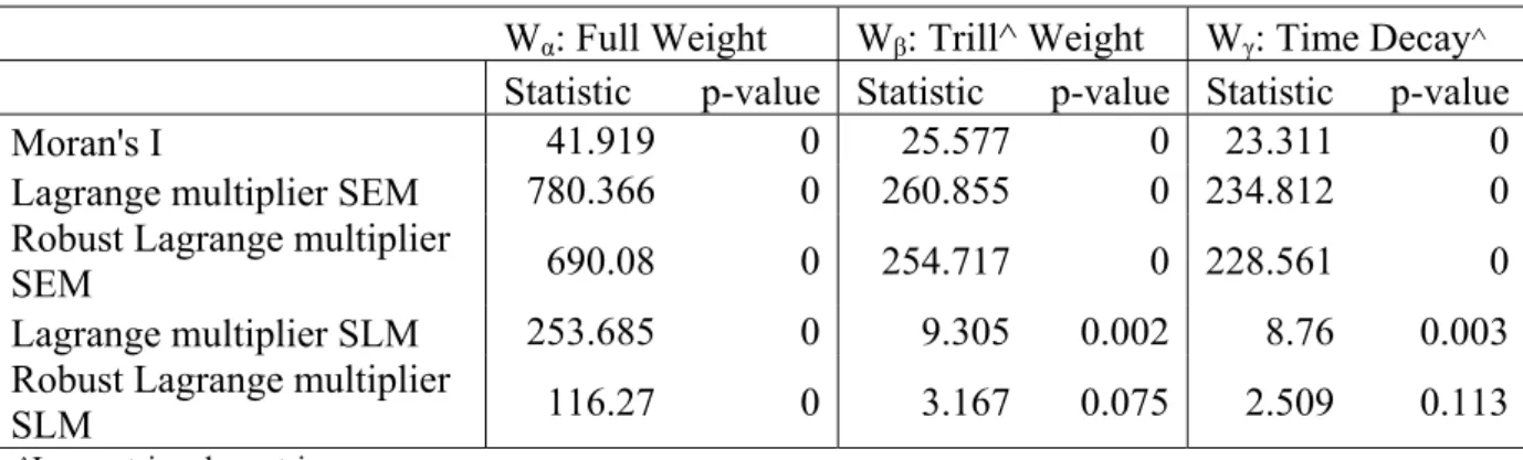
Table 2 presents these tests, where the null hypothesis in Moran’s I test of no spatial dependence is rejected in all models. However, the tests for selecting SLM or SEM are mo in
Testing the full weight matrix (W b
selecting one of the two. Interestingly this was also the finding of Chalermpong (2010) and Dekkers and Van der Straaten (2009) whose tests for both spatial lag and error are statistically significant in models that contain temporal ordering inconsistencies.
When the temporal ordering inconsistency is removed in weight matrix Wβ, the robust spatial lag test becomes insignificant, whereas the test for spatial error is still highly significant. This pattern is even more prominent in the weight matrix Wγ that includes time decay. Hence, we select the spatial error model. One inte
effects of a spatially lagged variable. In this context this would be house prices directly ffecting neighbouring prices, instead of the correct common exposure pattern.
a
Table 2: Spatial Dependence diagnostics
Wα: Full Weight Wβ: Trill^ Weight Wγ: Time Decay^ Statistic p-value Statistic p-value Statistic p-value
Moran's I 41.919 0 25.577 0 23.311 0
Lagrange multiplier SEM 780.366 0 260.855 0 234.812 0
Robust Lagrange multiplier
SEM 690.08 0 254.717 0 228.561 0
Lagrange multiplier SLM 253.685 0 9.305 0.002 8.76 0.003
Robust Lagrange multiplier
SLM 116.27 0 3.167 0.075 2.509 0.113
^Lower triangle matrix
As to the selection of an estimator, Maximum Likelihood (ML) estimation requires the assumption of normality (Cohen and Coughlin, 2008; Kim et al., 2003). The Jarque-Bera test (Jarque and Bera, 1987) cannot reject at the 99% level the null hypothesis of normality10 in the OLS residuals. Therefore, we use the ML estimator of Barry and Pace (1999) adapted and discussed in Franzese and Hays (2008), pointing out that the strictly lower triangular nature of Wβ and Wγ avoids the need to compute the determinant of a general matrix.
6.2. The HP Models Results
The HP model results are presented in Appendix 1. Looking at the OLS model, the fit to the data is excellent, explaining almost 87% of the variation. All the coefficients across the four models are of the expected sign and most are statistically significant at the 95% level. In all models, higher floor flats command a premium, as do detached houses and private garages. Conversely, houses in the non-coastal area or with lower room number are penalised. As xpected, the square meters of the floor space has a very significant positive effect on house
e
prices in our models. Being closer to schools, churches, the airport entrance and within 300 meters of the coastline positively affects prices. The distance to main roads coefficient is positive, possibly capturing accessibility advantages rather than traffic noise exposure. The price is negatively affected by proximity to plazas, which could be due to increased noise from human traffic and nightlife, and proximity to sport facilities, since these are mostly
Jarque-Bera statistic: 2.7339 (critical value: 5.
outdoor basketball courts and football grounds and tend to be on the fringe of the urban area. House age, proximity to public service buildings and hospitals do not have a statistically significant effect.
The aircraft noise coefficient in the OLS model produces a NDI of 0.646, which is in line with the HP literature (Nelson, 2004; Wadud, 2010). The most striking change between the LS and the ML1 model, which includes the temporal ordering inconsistency, is the fact that
ically ignificant aircraft noise coefficient of higher magnitude compared to ML1.
ation of distance effects. As expected, the structural ousing characteristics do not exhibit any substantial variation across models, being mostly
price levels ver time, which are often used to derive house price indices. Can and Megbolugbe (1997),
model, ML1, to fit the data better, albeit by overestimating spatial dependence due to the O
the aircraft noise coefficient is not statistically significant. This demonstrates that the temporal ordering inconsistency introduces overestimation of spatial dependence in a pattern that directly affects aircraft noise estimates. This is further supported by the results of ML2 and ML3 that correct for the temporal ordering inconsistency and produce a statist s
There is also a substantial reduction in the magnitudes of most of the distance effects in ML1 compared to OLS. The coefficients of “within 300 meters of the coastline”, “distance to church and main roads” lose statistical significance at the 95% level. In ML2 and ML3 distance effect estimates almost return to the OLS levels, implying that temporal ordering inconsistencies causes underestim
h
unaffected by spatial dependence and temporal ordering.
Looking at the quarterly dummies, OLS and ML1 exhibit very similar coefficient magnitudes, which increase significantly in ML2. The magnitudes of these coefficients are subsequently reduced in ML3, being very close to OLS and ML1 after 1999. The estimates of ML3 are considered the most reliable, since it incorporates the time decay factor that directly addressed the temporal aspect of spatial effects. These results show that the temporal ordering inconsistency or ignoring spatial dependence in HP affects the estimates of house
o
employing data from only a single quarter, did not examine such effects.
We employ the Akaike Information Criterion (AIC) and Bayesian Information Criterion (BIC) to compare the models with respect to overall goodness of fit. In the section 5.1 we mentioned that because Wα contains double the information of Wβ, we expect the equivalent
temporal ordering inconsistency. This is confirmed by both AIC and BIC, ML1 fits the data best compared to all other models.
More importantly, ML3, the model that incorporates time decay into the spatial dependence
pattern, provides a better fit to her e
time decay captures additio tio e ith t to
, rat ing it. C pared to ML2, there is an increase in the
se co t in ML wh r prefer e NDI
nt wi aircra noise ure that does not account for r tha .646 ND of our OLS model. However, we believe it imate for aircraft noise from a spatial HP model.
7. Conclusions
his paper has identified and defined the temporal ordering inconsistency found in
the data than eit ML2 or OLS. This d monstrates that the nal varia n in th data, w out con ributing spatial dependence overestimation her negat om
magnitude of the aircraft noi 0.493
efficien 3, ich is ou red model. Th of is broadly consiste th the HP ft literat
spatial dependence and lowe is the
n the 0 I
only robust est
In our data aircraft noise introduces on average 8.59 dBA above the 55dBA background noise. Given the 0.493 NDI from ML3, a complete removal of aircraft noise would also remove a depreciation of 8632.7€11 per house on average, if say the Airport was closed. It was actually closed on March 2001 and a new Athens International Airport started operations more than 20kms away in a more sparsely populated area.
T
sectional HP literature for valuing environmental commodities. The temporal ordering inconsistency leads to overestimation of spatial dependence, underestimating the effects of proximity to (dis)amenities and possibly the house price development over time. The Lagrange multiplier tests, employed as guidance for model selection, were also affected by this inconsistency. Spatial weight matrices have been developed to overcome this by ordering the data from the “furthest in the past” to the latest house sale, setting to zero all the values of the upper triangle square matrix and using only the lower triangle. Our preferred specification also introduces a time decay factor to the distance weights that specify the connection in space between the observations, directly addressing the temporal aspect of spatial effects.
11 This value refers to the base category (coastal area), for the non-coastal area the figures is 6705.1€. All
We note that Bateman et al. (2004) attributed the failure to produce statistically significant aircraft noise estimates to aircraft noise being less localised than other sources. Hence, these estimates were subsumed in their treatment of spatial effects. We agree with this observation nd we have shown that the temporal ordering inconsistency is responsible for subsuming
ur treatment of aircraft noise can also be considered a step forward, since it is not a crude
lly there is scope for improving the eatment of background noise. Although a common 55dBA assumption is not unreasonable
ith the GIS modelling and Robert Franzese and Jude Hays for their insight to spatial a
aircraft noise estimates in our data, leading to undervaluation of this externality.
Our preferred model with the time decay factor produced the best fit to the data among the models free from temporal ordering inconsistency, obtaining our preferred NDI estimate of 0.493. We consider this the first robust estimate of aircraft noise valuation from a spatial HP model. This is also the first HP study for Athens and Greece implying a potential benefit from the Airport closure of 8632.7€ per residential property in the study area at the time.
O
cut-off point that does not capture any effects below it. Our specification captures the effect of aircraft noise on the housing market above the general noise level in the area, even if aircraft noise effects are very low when dominated from other noise sources.
Clearly there are many areas for future investigation. We would like to test this approach on other data sets, developing further the specification of the time decay factor and combining it with different specifications of spatial weights. Additiona
tr
as an average for this data set it will clearly include under and over-estimations.
Acknowledgments
We would like to thank EUROCONTROL Experimental Centre for funding this research and especially Ted Elliff and Ian Fuller. We also owe thanks to Yiannis Kapanidis for his help w
dependence issues. The content of the paper and any opinions expressed are the sole responsibility of the authors.
Reference
Allen, J., Barlow, J., Leal, J., Maloutas, T., Padovani, L., 2004. Housing and Welfare in outhern Europe. Oxford, UK: Blackwell Publishing
nselin, L., 2002. Under the Hood: Issues in the Specification and Interpretation of Spatial
7–104
aranzini, A., Ramirez, J.V., 2005. Paying for quietness: the impact of noise on Geneva arry, R.P., Pace, R.K., 1999. Monte Carlo estimates of the log determinant of large sparse
on. ournal of Real Estate Finance and Economics, 14, 203-222
Chalermpong, S., 2010. Impact of Airport Noise on Property Values: Case of Suvarnabhumi International Airport, Bangkok, Thailand. Journal of the Transportation Research Board, S
Andersson, H., Jonsson, L., Ögren, M., 2010. Property Prices and Exposure to Multiple Noise Sources: Hedonic Regression with Road and Railway Noise. Environmental and Resource Economics, 45, 73–89
Anselin, L., 2010. Thirty years of spatial econometrics. Papers in Regional Science, 89, 3–25 Anselin, L., 2006. Spatial econometrics. In: T. Mills, K. Patterson, eds. Palgrave handbook of econometrics, vol. 1. In: Econometric Theory. Basingstoke: Palgrave Macmillan, 901-969 Anselin, L., 2003. Spatial externalities, spatial multipliers, and spatial econometrics. International Regional Science Review, 26, 153 – 166
A
Regression Models. Agricultural Economics, 27, 247 – 67
Anselin, L., 1988. Lagrange multiplier test diagnostics for spatial dependence and heterogeneity. Geographical Analysis, 20, 1–17
Anselin, L., Bera, A., Florax, R.J., Yoon, M., 1996. Simple diagnostic tests for spatial dependence. Regional Science and Urban Economics, 26, 7
B
rents. Urban studies, 42, 633–646 B
matrices. Linear Algebra and its Applications, 289, 41-54
Bateman, I., Day, B., Lake, I., Lovett, A., 2001. The effect of road traffic noise on residential property values: a literature review and hedonic pricing study. Scottish Executive Development Department, Edinburgh, UK
Bateman, I., Day, B., Lake, I., 2004. The valuation of transport-related noise in Birmingham. Non-technical report to Department for Transport, University of East Anglia, UK
Berglund, B., Lindvall, T., Schwela, D.H., 1999. Guidelines for Community Noise. World Health Organisation Geneva, Expert Task Force Meeting Guideline Document, April 1999, London, United Kingdom
Can, A., Megbolugbe, I., 1997. Spatial Dependence and House Price Index Constructi J
Charalampakis, G., 1980. Κοινωνική έρευναγύρω απότο Διεθνές Αεροδρόμιο Αθηνών (A social survey around Athens International Airport). Αρχιτεκτονική Ακουστική και ΠολεοδομικήΗχοπροστασία (Architectural Acoustics and Urban Noise Protection), 2, 209 – 215, Volos, Greece (article in Greek)
Cohen, J.P., Coughlin, C.C., 2008. Spatial hedonic models of airport noise, proximity, and ousing prices, Journal of Regional Science 48, 859–878
vironmental and Resource Economics, 37, 211–232
n. EEA Report o2/2010
ranzese, Jr. R. J., Hays, J.C., 2008. Empirical Models of Spatial Interdependence. In: J.M. ox-Steffensmeier, H. E. Brady, D. Collier, eds. The Oxford Handbook of Political
ethodology vol 7. Oxford, UK: Oxford University Press, 570-604
elfand, A.E., Ecker, M.D., Knight J.R., Sirmans C. F., 2004. The Dynamics of Location in rnal of Real Estate Finance and Economics, 29, 149-166
onic approach. Journal of Environmental Economics and anagement, 45, 24–39
h
Conway, D., Li, C.Q., Wolch, J., Kahle, C., Jerrett, M., 2010. A Spatial Autocorrelation Approach for Examining the Effects of Urban Greenspace on Residential Property Values. Journal of Real Estate Finance and Economics, 41:150–169
Day, B., Bateman, I., Lake, I., 2007. Beyond implicit prices: recovering theoretically consistent and transferable values for noise avoidance from a hedonic property price model. En
Dekkers, J.E.C., Van der Straaten, J.W., 2009. Monetary valuation of aircraft noise: A hedonic analysis around Amsterdam airport. Ecological Economics, 68, 2850–2858
European Environment Agency, 2010. Towards a resource-efficient transport system, TERM 2009: indicators tracking transport and environment in the European Unio
N
European Council, 2002. Directive 2002/30/EC on the establishment of rules and procedures with regard to the introduction of noise-related operating restrictions at Community airports. Official Journal of the European Communities, L 85/40
Fellmann, J.D, Getis, A., Getis, J., 2003. Human geography: landscapes of human activities. 7th ed. Boston: McGraw Hill
F B M G
Home Price. The Jou
Hui, E.C.M., Chau, C.K., Pun, L., Law, M.Y., 2007. Measuring the neighboring and environmental effects on residential property value: Using spatial weighting matrix. Building and Environment, 42, 2333–2343
Kim, C.W., Phipps, T.T., Anselin, L., 2003. Measuring the benefits of air quality improvement: a spatial hed
Miedema, H.M.E., 2007. Annoyance Caused by Environmental Noise: Elements for munity reaction to aircraft noise:
time-Statistical Data for Greece (in Greek) [online]. Evidence-Based Noise Policies. Journal of Social Issues, 63, 41-57
Miedema, H.M.E., Vos, H., De Jong, R.G., 2000. Com
of-day penalty and trade off between levels of overflights. Journal of the Acoustical Society of America, 107, 3245–3253
National Statistical Service of Greece, 2003.
General Secretariat of National Statistical Service of Greece, Ministry of Economy and Finance, Piraeus, Greece. Available from:
http://www.statistics.gr/StatMenu.asp [accessed on 22/10/2005]
Nelson, J. P., 1980. Airports and property values: a survey of recent evidence. Journal of Transport Economics and Policy, 14, 37–52
Nelson, J. P., 2004. Meta-analysis of airport noise and hedonic property values: problems and prospects. Journal of Transport Economics and Policy, 38, 1 – 28
chaerer, P. Thalman, eds. Hedonic Methods
bos
Nelson, J. P., 2008. Hedonic Property Value Studies of Transportation Noise: Aircraft and Road Traffic. In: A. Baranzini, J. Ramirez, C. S
in Housing Markets, vol. 3. In: Pricing Environmental Amenities and Segregation. New York, USA: Springer, 55-82
OECD, 2006. Consumer Price Index for Housing [online]. Available from OECD StatExtracts: http://stats.oecd.org/w [accessed on 23/09/2008]
inance and Economics, 17, 15-33
mics of Time to Sale. Real Estate Economics. 34, Journal of
onomics and Statistics, 2008-IV-3, 577–606.
– 124
Pace, R. K., Barry, R., Clapp, J.M., Rodriguez, M., 1998. Spatiotemporal Autoregressive Models of Neighborhood Effects. Journal of Real Estate F
Palmquist, R. B., 1992. Valuing Localized Externalities. Journal of Urban Economics, 31, 59-68
Pryce, G., Gibb, K., 2006. Submarket Dyna 377–415
Rich, J.H., Nielsen, O.A., 2004. Assessment of traffic noise impacts, International environmental studies. 61, 19–29
Salvi, M., 2008. Spatial Estimation of the Impact of Airport Noise on Residential Housing Prices. Swiss Journal of Ec
Schipper, Y., Nijkamp, P., Rietveld P., 1998. Why do aircraft noise value estimates differ? A meta-analysis. Journal of Air Transport Management, 4, 117
Taylor, S.M., Hall, F.L., Birnie, S.E., 1987. Transportation noise annoyance: testing of a probabilistic model. Journal of Sound and Vibration, 117, 95–113
Thanos, S., Wardman, M.R., Bristow, A.L., 2011. Valuing aircraft noise: Stated Choice experiments reflecting inter-temporal noise changes from airport relocation. Environmental and Resource Economics, 50, 559-583.
Theebe, M.A., 2004. Planes, trains, and automobiles: the impact of traffic noise on house an growth in the Detroit region,
258
prices. Journal of Real Estate Finance and Economics, 28, 209–234 Tobler, W., 1970. A computer movie simulating urb
Economic Geography, 46, 234–240
Tomkins, J., Topham, N., Twomey, J., Ward, R., 1998. Noise versus access: The impact of an airport in the urban property market. Urban Studies, 35, 243
-Wadud, Z., 2010. Meta-Regression of NDIs around Airports: Effect of Income/Wealth, paper presented at the 12th World Conference on Transport Research, 11th to 15th July 2010, Lisbon, Portugal
Watkins, C. A., 2001. The definition and identification of housing submarkets. Environment and Planning A. 33, 2235 – 2253
White M., Watkins, C. A., 2004. Spatial, house-type and temporal variations in time on the market. Presented at the 11th European Real Estate Society Conference, 2nd to 5th June 2004, Milan, Italy
Zuehlke, T.W., 1987. Duration dependence in the housing market. The Review of Economics and Statistics, 69, 701 - 709
Appendix 1: The HP Models Model OLS ML1: Full Weight (Wα) ML2: Trill Weight (Wβ) ML3: Time Decay (Wγ)
Variable Name Coef. Coef. Coef. Coef.
Lden_tot -0.00646*** -0.00196 -0.00454*** -0.00493*** (0.00135) (0.00137) (0.00136) (0.00135) sq meters 0.00421*** 0.00427*** 0.00425*** 0.00422*** (0.00016) (0.00015) (0.00015) (0.00015) room1_2 -0.68726*** -0.68876*** -0.68642*** -0.68121*** (0.02247) Base Base (0.01999) 0.25723*** (0.01884) (0.01921) (0.01920) Base
4 Base Base Base Base
d 0.12209*** 0.12566*** 0.12014*** 0.12238*** ched 0.05518** 0.04408* 0.05755** 0.05690** .09136*** 0.08726*** 0.08608*** (0.02793) -8.2E-05*** (1.9E-05) (2.1E-05)
d_plaza -1.3E-04*** -9.4E-05*** -1.2E-04*** -1.2E-04***
(0.02303) (0.02202) (0.02246)
room3 -0.29225*** -0.29934*** -0.29291*** -0.28759***
(0.01791) (0.01714) (0.01746) (0.01747)
room4 Base Base
room5 0.18547*** 0.19445*** 0.18818*** 0.19133*** (0.02048) (0.01961) (0.01998) room6 0.25689*** 0.26040*** 0.25773*** (0.02409) (0.02304) (0.02349) (0.02348) room7 0.28137*** 0.28589*** 0.28617*** 0.28986*** (0.02756) (0.02636) (0.02688) (0.02690) House>10yr -0.01933 -0.02075 -0.01945 -0.01897 (0.01970) House 6-9yr -0.01657 -0.01235 -0.01439 -0.01551 (0.01784) (0.01707) (0.01740) (0.01739)
H_Age_B Base Base Base
floors_7-8 0.05676 0.10853** 0.07231 0.06387 (0.05249) (0.05047) (0.05126) (0.05117) floors_4-6 0.09369*** 0.11069*** 0.10019*** 0.09867*** (0.01450) (0.01398) (0.01419) (0.01416) floors< detache (0.02392) (0.02287) (0.02332) (0.02331) semideta (0.02432) (0.02328) (0.02372) (0.02370)
flat Base Base Base Base
garage 0.08984*** 0
(0.01231) (0.01178) (0.01201) (0.01202)
non_coastal -0.24926*** -0.35083*** -0.30166*** -0.26541***
(0.02852) (0.02915) (0.02931)
Coastal_area Base Base Base Base
d_ sports -9.1E-05*** -6.0E-05*** -8.4E-05***
(1.9E-05) (1.8E-05) (1.9E-05)
d_public_serv 1.2E-05 -5.3E-06 8.9E-06 6.9E-06
Model OLS ML1: Full Weight (Wα) ML2: Trill Weight (Wβ) ML3: Time Decay (Wγ)
Variable Name Coef. Coef. Coef. Coef.
(3.0E-05) (2.9E-05) (2.9E-05) (2.9E-05)
d_school 1.7E-04*** 1.1E-04*** 1.6E-04*** 1.5E-04***
(2.4E-05) (2.3E-05) (2.3E-05)
d_supermarket -4.1E-05*** -2.8E-05** -3.8E-05***
(2.3E-05)
-3.6E-05***
E-05* 6.6E-05** 6.4E-05**
(1.4E-05)
(6.7E-06) (6.5E-06) (6.6E-06) (6.6E-06)
0.38219*** -0.67981*** -0.53115*** -0.50644*** -0.51521*** -0.79166*** -0.61010*** (0.03714) (0.06121) (0.04060) -0.43064*** -0.68209*** -0.50894*** (0.03477) (0.03326) (0.05706) (0.03704) -0.45616*** -0.69755*** -0.52558*** (0.03602) (0.03445) (0.05613) (0.03747) -0.49430*** -0.73431*** -0.56531*** (0.03476) (0.03325) (0.05346) (0.03569) -0.38464*** -0.60548*** -0.44081*** (0.03861) (0.03693) (0.05418) (0.03885) -0.28249*** -0.49446*** -0.34503*** (0.03674) (0.03513) (0.05210) (0.03751) -0.33851*** -0.53784*** -0.39293*** (0.03533) (0.03379) (0.04984) (0.03591) -0.30098*** -0.48805*** -0.34601*** (0.03354) (0.03207) (0.04661) (0.03364) -0.37546*** -0.55582*** -0.42096*** (0.04270) (0.04084) (0.05181) (0.04218) y98q1 -0.24365*** -0.21938*** -0.40130*** -0.30476*** (0.03734) (0.03579) (0.04583) (0.03789) y98q2 -0.23354*** -0.24206*** -0.39512*** -0.29039*** (0.03131) (0.02995) (0.04179) (0.03205)
(1.4E-05) (1.3E-05) (1.4E-05) (1.4E-05)
d_church 8.1E-05*** 4.8
(2.7E-05) (2.6E-05) (2.6E-05) (2.6E-05)
d_health -1.9E-05 -1.8E-05 -2.4E-05* -2.2E-05
(1.4E-05) (1.4E-05) (1.4E-05)
d_main_rd 9.3E-05*** 4.5E-05 6.6E-05** 7.1E-05**
(3.1E-05) (3.0E-05) (3.1E-05) (3.1E-05)
d_air_4km 3.2E-05*** 2.8E-05*** 3.6E-05*** 3.1E-05*** Akto_300m 0.04203** 0.02831 0.03873** 0.03561** (0.01854) (0.01779) (0.01809) (0.01810) y95q1 -0.37105*** (0.03636) (0.03479) (0.06503) (0.04491) y95q2 -0.47472*** -0.48113*** -0.77176*** -0.59768*** (0.03594) (0.03437) (0.06308) (0.04094) y95q3 (0.03517) (0.03364) (0.06093) (0.03865) y95q4 -0.45703*** -0.46232*** -0.72939*** -0.54233*** (0.03883) y96q1 -0.42217*** y96q2 -0.44960*** y96q3 -0.50018*** y96q4 -0.38484*** y97q1 -0.28022*** y97q2 -0.33387*** y97q3 -0.29993*** y97q4 -0.38116***
ML1: Full Weight (Wα) ML2: Trill Weight (Wβ) ML3: Time Decay (Wγ) Model OLS
Variable Name Coef. Coef. Coef. Coef.
y98q3 -0.18221** -0.17426** -0.32412*** -0.22529*** (0.07129) 49*** 0*** 75*** 2*** 9q1 * * * * 9q2 * * * * 9q3 * * * * 9q4 * * * * 24) 15) 96) 58) nstant mbda (0.06818) (0.07389) (0.06987) y98q4 -0.208 -0.2107 -0.345 -0.2549 (0.03164) (0.03025) (0.03923) (0.03185) y9 -0.10104** -0.11242** -0.22458** -0.11354** (0.02739) (0.02621) (0.03448) (0.02678) y9 -0.16852** -0.16902** -0.26490** -0.15325** (0.02923) (0.02796) (0.03320) (0.02861) y9 -0.17800** -0.19939** -0.26714** -0.17786** (0.04334) (0.04150) (0.04509) (0.04223) y9 -0.21614** -0.23333** -0.29831** -0.24284** (0.071 (0.068 (0.070 (0.069 y00q1 -0.03739 -0.05575** -0.11391*** -0.07356*** (0.02727) (0.02615) (0.02983) (0.02730) y00q2 -0.04355 -0.05826** -0.09467*** -0.03048 (0.02817) (0.02698) (0.02891) (0.02755) y00q3 -0.08003** -0.08448** -0.11089*** -0.06170* (0.03595) (0.03438) (0.03547) (0.03518)
y00q4 Base Base Base Base
co 12.134*** 12.229*** 12.315*** 12.225*** 0.09447) 0.09085) 0.09752) (0.09339) la 0.0107*** 0.0095*** 0.0292*** (0.00109) 69) 04) * * (0.001 (0.005 sigma 0.2052*** 0.2093** 0.2092** Wald χ (48) inal LL 2 ared 11738*** 11158*** 11040*** F 265.22 233.93 234.70 Adj R-squ 0.868 AIC IC -338.11 -428.44 -365.86 -367.40 B -74.12 -153.76 -91.18 -92.73
*** significant at p < 0.01; ** sig p < 0.05; t at p < 0.1 Standard error in t
nificant at * significan he brackets