OBJECT-RELATIONAL DATA
by
Fatemeh Riahi
MSc, Dalhousie University, 2012 BSc, Sharif University of Technology, 2009 a Thesis submitted in partial fulfillment
of the requirements for the degree of
Doctor of Philosophy in the
School of Computing Science Faculty of Applied Sciences
c
Fatemeh Riahi 2016 SIMON FRASER UNIVERSITY
Fall 2016
All rights reserved.
However, in accordance with theCopyright Act of Canada, this work may be reproduced without authorization under the conditions for “Fair Dealing.” Therefore, limited reproduction of this work for the purposes of private study,
research, criticism, review and news reporting is likely to be in accordance with the law, particularly if cited appropriately.
Name: Fatemeh Riahi
Degree: Doctor of Philosophy
Title of Thesis: Model-based Outlier Detection for Object-Relational Data
Examining Committee: Dr. Ramesh Krishnamurti, Professor, Computer Science Chair
Dr. Oliver Schulte, Professor, Computing Science Senior Supervisor
Dr. Jian Pei, Professor, Computing Science Supervisor
Dr. Christos Faloutsos, Professor, Computer Science Carnegie Mellon University
External Examiner
Dr. David Mitchell
Associate Professor, Computing Science Internal Examiner
Date Approved:
Outliers are anomalous and interesting objects that are notably different from the rest of the data. The outlier detection task has sometimes been considered as removing noise from the data. However, it is usually the significantly interesting deviations that are of most interest.
Different outlier detection techniques work with various data formats. The outlier detec-tion process needs to be sensitive to the nature of the underlying data. Most of the previous work on outlier detection was designed for propositional data. This dissertation focuses on developing outlier detection methods for structured data, more specifically object-relational data. Object-relational data can be viewed as a heterogeneous network with different classes of objects and links.
We develop two new approaches to unsupervised outlier detection; both approaches leverage the statistical information obtained from a statistical-relational model. The first method develops a propositionalization approach to summarize information from object-relational data in a single data table. We use Markov Logic Network (MLN) structure learning to construct the features for the single data table and to mitigate the loss of infor-mation that usually happens when features are generated by manual aggregation. By using propositionalization as a pipeline, we can apply many previous outlier detection methods that were designed for single-table data.
Our second outlier detection method ranks the objects as potential outliers in an object-oriented data model. Our key idea is to compare the feature distribution of a potential outlier object with the feature distribution of the objects class. We introduce a novel distribution divergence concept that is suitable for outlier detection. Our methods are validated on synthetic datasets and on real-world data sets about soccer matches and movies.
First I want to thank my Ph.D. senior supervisor, Dr. Oliver Schulte. I appreciate all his contributions of time, ideas, and funding that made my Ph.D. possible. I am very thankful for his excellent guidance, knowledge and patience throughout my Ph.D. I would also like to thank my supervisor, Dr. Jian Pei for his guidance and support. I am grateful to Dr. Christos Faloutsos and Dr. David Mitchell for participating in my final defense as external and internal examiners.
I gratefully acknowledge my collaborators and other students that I had a chance to work with during my Ph.D., Nicole Li, Zhensong Qian, Sajjad Gholami, Yan Sun and Mahmoud Khademi.
I would like to thank my friends that made my student life more enjoyable: Anahita, Elaheh, Mojtaba, Monir, Ali M., Shabnam, Atieh, Ali R. and Faezeh.
Last but not least, I am deeply appreciative of the support given to me by my family. I would especially like to thank my father and mother for all the sacrifices that they have made on my behalf. And most of all I would like to thank my loving, supportive and patient husband Ali. He has been my motivation to move my career forward.
Approval ii Abstract iii Dedication iv Quotation v Acknowledgments vi Contents vii List of Tables x
List of Figures xii
1 Introduction 1
1.1 Outlier Definition . . . 1
1.1.1 Outlier Detection Challenges . . . 2
1.1.2 Approach . . . 3
1.1.3 Contributions . . . 6
1.1.4 Limitations and Directions for Future Work . . . 6
2 Literature Review 9 2.1 Outlier Detection Methods for Propositional Data . . . 10
2.1.1 Supervised Methods for Propositional Data . . . 10
2.1.2 Unsupervised Methods for Propositional Data . . . 12
2.3 Outlier Detection Methods for Relational Data with non-propositional
Ap-proach . . . 20
2.3.1 Supervised . . . 20
2.3.2 Unsupervised . . . 21
2.4 Outlier Detection Methods for Other Types of Structured Data . . . 24
2.5 Limitations of Current Outlier Detection Methods . . . 24
3 Background, Data Model and Statistical Models 26 3.1 Notation and Definition . . . 26
3.2 Object-relational Data Model . . . 28
3.3 Synthetic Datasets . . . 31
3.4 Real-world Datasets . . . 31
3.5 Statistical Models . . . 34
3.5.1 Bayesian Network . . . 34
3.5.2 Markov Logic Network . . . 35
3.5.3 Structure Learning . . . 36
3.6 Evaluation Techniques in Outlier Detection . . . 37
4 Propositionalization for Outlier Detection 39 4.1 Introduction . . . 40
4.2 Propositionalization, Pseudo-iid Data Views, and Markov Logic Networks . . 42
4.3 Wordification: n-gram Methods . . . 45
4.4 Propositionalization methods and Feature functions . . . 45
4.5 Experimental Design: Methods Used . . . 46
4.6 Evaluation Results . . . 47
4.6.1 Performance Metrics Used . . . 47
4.6.2 Dimensionality of Pseudo-iid Data Views . . . 48
4.6.3 Accuracy . . . 48
4.7 Comparison With Propositionalization for Supervised Outlier Detection and Log-Likelihood . . . 53
4.8 Conclusion . . . 54
5.2 Related Work . . . 59
5.3 Likelihood-Distance Object Outlier score . . . 60
5.3.1 Motivation . . . 62
5.3.2 Comparison Outlier Scores . . . 63
5.4 Comparison with Other Dissimilarity Metrics . . . 65
5.5 Two-Node Examples . . . 66 5.5.1 Computations . . . 66 5.5.2 Visualization . . . 68 5.6 Experimental Design . . . 70 5.6.1 Methods Compared . . . 70 5.7 Empirical Results . . . 70 5.8 Conclusion . . . 75
6 Success and Outlierness 78 6.1 Introduction . . . 78
6.2 Preliminary Analysis . . . 79
6.3 Related Work . . . 81
6.3.1 Analyzing Sports Data . . . 81
6.3.2 Ranking system in Sports Domain . . . 82
6.4 Correlation with Success . . . 82
6.4.1 Methodology . . . 83
6.4.2 Correlations between theELD outlier metric and success . . . 84
6.5 Conclusion . . . 88
7 Summary and Conclusion 91
Bibliography 93
3.1 Table of Notations . . . 27
3.2 Sample population data table (Soccer). . . 28
3.3 Sample object data table, for teamT =WA. . . 28
3.4 Example of grounding count and frequency in Premier League . . . 29
3.5 Instances of the conjunction: passEff(T,M) =high∧shotEff(T,M) =high∧ Result(T,M) =win in the network representation of Figure 3.2. . . 29
3.6 Attribute features. . . 32
3.7 Summary statistics for the IMDb and the Premier League datasets . . . 33
3.8 Outlier/normal objects in real-world datasets. . . 34
3.9 MLN formulas derived from the toy Bayesnet shown in Figure 3.4 . . . 36
4.1 An example pseudo-iid data view. . . 43
4.2 Generating pseudo-iid data views using Feature Functions and Formulas . . 46
4.3 OutRank running time (ms) given different attribute vectors. . . 50
4.4 Summarizing the accuracy results of Figures 4.4 and 4.3 . . . 50
4.5 Accuracy of Treeliker for different databases and outlier techniques . . . 54
5.1 Example of grounding count and frequency in the Premier League data, for the conjunctionpassEff(T,M) =hi,shotEff(T,M) =hi,Result(T,M) =win. 59 5.2 Baseline comparison outlier scores . . . 64
5.3 Example computation of different outlier scores for outliers given the distri-butions of Figure 5.3 (a),(b). . . 67
5.4 Time (min) for computing theELD score. . . 71
5.5 The Bayesian network representation decreases the number of terms required for computing theELD score. . . 71
5.8 Case study for the top outliers returned by the log-likelihood distance score
ELD . . . 76
6.1 Average salary of players in different teams . . . 80
6.2 Success metrics and their distributions. . . 83
6.3 Correlation betweenELD metric and success metric of Movies. . . 84
6.4 Correlation betweenELD metric and standing of Teams. . . 84
6.5 Correlation betweenELD metric and success metrics of Players. . . 84
6.6 Comparison of two midfielders. . . 86
1.1 Categorization of outlier detection methods. . . 3
1.2 A tree structure for research on outlier detection for structured data. . . 6
2.1 Related work categorization . . . 9
2.2 Advantage of using Mahalanobis distance functio . . . 14
2.3 Outliers with respect to subspace views. . . 16
2.4 Impact of local density on outliers . . . 17
2.5 Dotted circles show the distance to each point’s third nearest neighbour. . . . 18
2.6 ego and ego-net in a toy graph. . . 20
3.1 An example database . . . 29
3.2 Conjunction instantiation in the network representation . . . 30
3.3 Illustrative Bayesian networks . . . 32
3.4 Example of joint and marginal probabilities computed from a toy Bayesian network structure. . . 35
3.5 Learning an Markov Logic Network from an input relational database. . . . 37
4.1 System Flow . . . 42
4.2 Comparison of complexity, dimensionality and construction time (min) for the attributes produced by different propositionalization methods . . . 49
4.3 Accuracy for different Methods and Attribute Vector in the Synthetic datasets 51 4.4 Accuracy for different Methods and Attribute Vector in the Real World datasets 52 5.1 Computation of outlier score. . . 58
5.2 A tree structure for related work on outlier detection for structured data. . . 59
5.3 Illustrative Bayesian networks with two nodes. . . 68
6.1 Salary comparison of Premier League Players . . . 81
6.2 Team Standing vs. ELD for the top teams in the Premier League. . . 85
6.3 Correlations in the strikers population . . . 87
6.4 Correlations in the goalies population . . . 88
6.5 Correlation in the movies population . . . 89
Introduction
Detection of outliers is an essential part of knowledge discovery in databases (KDD) and has been used to identify anomalous entities from data for decades. System faults or changes, human or mechanical error, or any sort of deviations in population may result in outliers in the data [37].
Many techniques have been employed in Data Mining, Machine Learning, and Statistics to find outliers in different domains such as Network Performance, Motion Segmentation, Medical Condition Monitoring and Pharmaceutical Research. Demand for efficient analy-sis methods to detect outliers has increased due to the large amount of data collected in databases. In this dissertation, we developed two generative model-based methods for the case of object-relational data.
1.1
Outlier Definition
Many definitions have been proposed for an outlier and there is no generally accepted defini-tion. Grubbset al. define an outlier as an observation that appears to deviate considerably from other members of the sample in which it occurs [33]. Hawkings et al. describe an outlier as an observation which deviates so much from the other observations as to arouse suspicions that it was generated by a different mechanism [35]. These are only a few exam-ples of definitions proposed in the previous outlier detection work. Essentially, the outlier definition is context-related and depends on the type of the application that employs the outlier detection. For example, Akogluet. aldefine outliers in graphs as rare graph objects that differ significantly from the majority of the reference objects in the graph [5]. This
definition is the basis of our proposed outlier detection methods.
The output of an outlier detection algorithm can be one of these two types [3]:
1. Outlier score assigned to each individual that shows the degree of “outlierness” of each data point.
2. A binary label indicating whether a data point is an outlier or not. By imposing thresholds on outlier scores, based on their statistical distribution, the outlier scores can be converted into binary labels.
1.1.1 Outlier Detection Challenges
Outlier Detection applications must overcome many challenges. For example:
• Modeling normality is hard: there is not often a clear line separating data normality and abnormality since it is hard to define all possible normal behaviours. Therefore, many outlier techniques measure the degree of outlierness of each data point instead of firmly labelling it as either outlier or normal.
• Designing an outlier detection method depends on the type of application: one of the earliest steps in designing a model to identify outliers is choosing a similarity or distance measure. However, different applications require different sensibility in terms of similarity or difference. For example, in medical data analysis, a tiny deviation may be a sign of an outlier; while marketing analysis, for example, allows larger fluctuations between its normal data points.
• Separating noise and error from the outliers: outliers and noise are different, however, they are similar in the sense that they both deviate from the normal behaviour. This similarity can make the distinction between normal and outlier and noise objects even harder.
• Understandability and interpretability: in some applications, detected outliers should be justified and the features that moved the data points from normal to outlier should be identified. In this case, outlier detection methods must provide explanations.
• Class imbalance: the imbalanced nature of outlier detection makes accurate detection hard to achieve.
1.1.2 Approach
Many outlier detection methods have been developed for data that are represented in a propositional format (i.e., as a flat feature vector) or unstructured data.
Related Work
Outlier Detection
in
Static Data
Outlier Detection
in Dynamic Data
Input Format: Propositional Data Input Format: Structured DataPlain Attributed Plain Attributed
● Probabilistic, Generative model-based and Statistic-based Methods
● Proximity-based Methods and Feature-based Methods ● Community-based
● Relational Learning-based
Out of Scope of this Dissertation
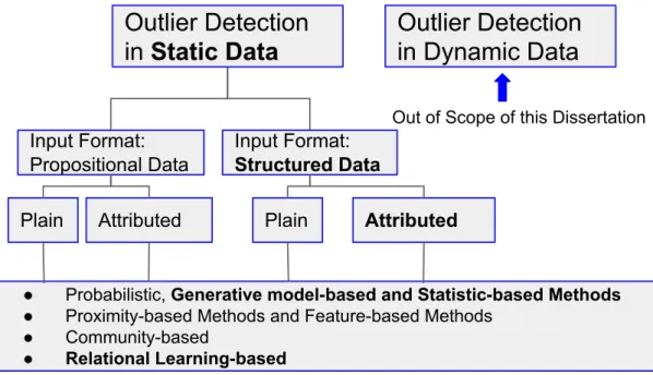
Figure 1.1: Categorization of outlier detection methods. The bold font indicates where our methods stand in this categorization.
In a propositional data table, a row represents a data point, a column represents an attribute of a data point, and a table entry represents an attribute value for a data point. This dissertation extends unsupervised statistical outlier detection to the case of structured data, more specifically object-relational data. Object-relational data represents a complex heterogeneous network [29], which comprises objects of different types, links among these objects, also of different types, and attributes of these links. Given the prevalence of object-relational data in organizations, outlier detection for such data is an important problem in practice. However, applying standard outlier detection methods designed for single data tables on object-relational data runs into impedance mismatch, since object-relational data are represented in multiple interrelated tables.
model-based approaches. The advantages of employing a model-based approach for outlier detection are as follows: 1) We can apply many statistical relational learning methods for building the model. 2) We can leverage statistical concepts such as divergence metrics to measure outlierness of the data points. 3) We can employ outlier detection methods de-signed for the propositional data.
A disadvantage of using a generative model is the possibility that model overfits the data, meaning that the model has low error on the training data but poor predictive performance on unobserved data. To avoid overfitting, the Bayesian network learning algorithm that we use in this work utilize a standard complexity penalty. Furthermore, poor predictions are not an issue in our specific task as we employ the generative model for the descriptive statistics and not for a specific prediction task. According to Aggarwal [3], if a generative model overfits the data it will also find a way to fit the outliers. The performance of our outlier detection methods shows that overfitting did not happen in our experiments.
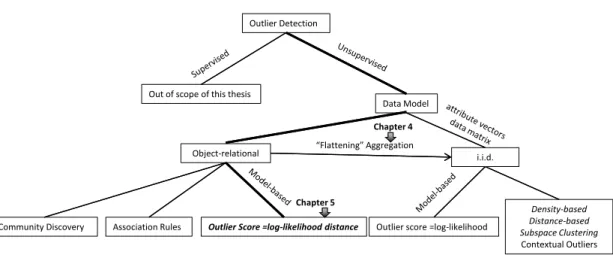
Based on the categorization of Figure 1.1, our proposed outlier detection methods fall into the category of unsupervised, relational learning-based, attributed models which can be applied to both static and dynamic datasets. The two methods are:
1. In chapter 4 a model-based method is proposed to generate conjunctive features for outlier detection. This method leverages outlier detection tools that are designed for a single table via a pipeline data preprocessing approach by converting the object-relational data into a single attribute-value table, then applying the data analysis tools. Since the attribute value representation corresponds to propositional logic, the conversion is called propositionalization. Propositionalization has been used to detect outliers in the literature. For example, a technique called ODDBALL introduced by Akogluet al. extracts graph-centric features to detect anomalies in graph structure [5]. However, to the best of our knowledge, our work is the first model-based propositional-ization approach for outlier detection. In Chapter 4 we show that conjunctive features for outlier detection can be learned from data by using statistical-relational meth-ods. Specifically, we apply the Markov Logic Network structure learning method to construct the features. Compared to baseline propositionalization methods, Markov Logic propositionalization produces the most compact data tables, whose attributes
capture the most complex relational correlations. We apply three representative out-lier detection methods (LOF,KNNOutlier,OutRank) to the data tables constructed by propositionalization.
This research was published in the proceedings of the Florida Artificial Intelligence Association (FLAIRS2016) conference [26].
2. Chapter 5 introduces a model-based method to define an outlierness metric. We first apply state-of-the-art probabilistic modelling techniques for object-relational data that construct a graphical model (Bayesian network), which compactly represents probabilistic associations in the data. We propose a new metric, based on the learned object-relational model, that quantifies the extent to which the individual association pattern of a potential outlier deviates from that of the whole population. The metric is based on the likelihood ratio of two parameter vectors: One that represents the population associations, and another that represents the individual associations. Our method is validated on synthetic datasets and on real-world datasets about soccer matches and movies. Compared to the baseline methods, our novel likelihood-based model achieved the best detection accuracy on all datasets except one.
Model-based methods have been previously used for outlier detection tasks. Loglike-lihood has been used to identify outliers [14]. Rule mining and sub-group mining are other examples of model-based outlier detection [4, 47]. However, none of these methods are based on a joint distribution distance metric.
This work was published in the proceedings of IEEE Symposium series on Computa-tional Intelligence (SSCI 2015) conference and won the best student paper award [76]. In chapter 6 we compare the log-likelihood distance to metrics of success for a given do-main. Success rankings are one of the most interesting features to users. Our reasoning is that high success is an independent metric that indicates an unusual individual. So a correlation between log-likelihood distance and success is an independent validation of the log-likelihood distance, and also shows that this metric points to meaningful and interesting outliers. A version of this work has been submitted to the Journal of Data mining and Knowledge discovery.
Figure 1.2 provides a tree diagram of where our methods are situated with respect to other outlier detection methods and other data models.
Outlier Detection
Out of scope of this thesis
Object-relational Association Rules Density-based Distance-based Subspace Clustering Contextual Outliers
Community Discovery Outlier Score =log-likelihood distance
Chapter 5
Data Model
i.i.d. “Flattening” Aggregation
Outlier score =log-likelihood Chapter 4
Figure 1.2: A tree structure for research on outlier detection for structured data. A path specifies an outlier detection problem, the leaves list major approaches to the problem.
1.1.3 Contributions
The main contributions of this dissertation are the following:
1. The first approach to outlier detection for structured data that is based on a proba-bilistic model.
2. A new model-based outlier score based on a novel model likelihood comparison, the log-likelihood distance.
3. A novel task for relational learning: MLN-propositionalization for outlier detection. This facilitates leveraging standard single-table outlier analysis methods for object-relational data. This task is also a novel application of Markov Logic Network structure learning.
4. A novel task for relational learning: propositionalization for outlier detection. This fa-cilitates leveraging standard single-table outlier analysis methods for object-relational data. We use Markove Logic Network (MLN) structure learning for propositionaliza-tion. This is a novel application of MLN structure learning.
1.1.4 Limitations and Directions for Future Work
1. Limitation of Approach:
(a) Our proposed methods rank potential outliers, but do not set a threshold for a binary identification of outlier vs. non-outlier.
(b) Our current Bayesian Network Learning method can only be applied to discrete data. Prior to learning the model, we take an extra step in data preprocessing and convert continuous data into discrete, which naturally causes some information loss.
(c) Our generative model-based methods learn a generic Bayesian network structure for the entire population, ignoring the subgroups that inherently exist in the real datasets, as a result, the detected outliers are global outliers. However, there are more complex outliers that locally deviate from their subgroups and can be detected only by subgroup comparison. One direction for future work is to first detect subgroups in the population and then perform the outlier detection task. 2. Limitation of Data Analysis:
In this dissertation, to simplify the outlier detection task, we used only part of the full information available in our rich datasets. The model-based outlier detection can be extended in future work to take advantage of the full information.
(a) In the Premier League dataset, players are naturally related to one another and modelling the interaction between players can be another way to detect anoma-lous players. The graph-based features, such as detecting near-clique nodes and star nodes, proved to be efficient in discovering patterns for anomaly detection task as shown in ODDBALL [5].
(b) In this dissertation we did not use the temporal information available in the data. In the learning process we do not give a higher weight (importance) to the more recent action (performance) of an individual. This point is especially important when applying the methods to dynamic data or the data that are collected from long periods of time.
(c) In the datasets that we used for the experiments, we did not have the missing value problem. Therefore, we did not incorporate ways to estimate missing values in our modeling. However, real-world datasets may involve arbitrary pattens of
missing data. Maximum likelihood density estimation is a way to estimate such values. We leave this feature for future work.
Literature Review
This chapter provides a literature review of the state-of-the-art methods in the field of outlier detection. Outlier detection is a very well-explored area and there are many surveys to overview the state-of-the-art methods. Each survey categorized these methods differently [6, 3, 37]. The categorization can be based on datatype (e.g. graph data) or type of methods that have been used to detect outliers (e.g. structured-based methods). In this chapter we group outlier methods based on the format of the input data, whether it is presented in a single data table or it has a higher level of organization such as data presented in a relational database, or XML format or OLAP. Since the focus of our work is on structured data, we mainly concentrate on the methods designed for that data format .
We conclude this chapter with section 2.5 which addresses the limitations of current outlier detection methods. Figure 2.1 shows the organization of this chapter.
Outlier Detection in Propositional Data Outlier Detection in Structured Data Relational Data Propositional Approach Non-Relational Data- Propositional Approach Relational Data- Non-propositional approach
Other type of Structure: XML-OLAP:Non-proposition al approach
Figure 2.1: Related work categorization
2.1
Outlier Detection Methods for Propositional Data
In this section we explore outlier detection methods that takepropositional data. One inter-pretation of propositional data is that the attributes describe characteristics of one object-class. For example,shotEfficiency(Player) shows shot efficiency of a player in general, while in the structured data the attributes are more complex; for example in the Object-relational data model, the attributes are shown in this format: shotEfficiency(Player,Match) which represents shot efficiency of a player in a match and involves two object-classes. Throughout this dissertation, we refer to the methods designed for a single data table as propositional methods. In this section, we further categorize these methods into supervised and unsu-pervised based on whether the sample of data has been provided with labels and domain expert information to build an outlier detection model.
2.1.1 Supervised Methods for Propositional Data
These methods model both normality and abnormality and require pre-labelled data. Nor-mal points may belong to a single class or be divided among different classes. Supervised outlier detection is a special case of the classification where the labels are extremely un-balanced in terms of occurrence [15]. Normal data points are easily available while outlier examples are very sparse and it is the rarity that makes these data points outliers. In this sense, outlier detection can also be viewed asrareclass detection problem. The imbalanced nature of outlier detection makes the accurate classifications quite hard to achieve and might result in over-training [3].
When the purpose of classification is outlier detection, cost-sensitive variations of ma-chine learning algorithms can be used in order to make the classification of anomalies more accurate [3]. Class imbalance is one of the common problems in supervised outlier detection. The standard evaluation techniques in classification cannot simply be applied to outlier de-tection. For example, in the case of breast cancer, where 99% of scans are identified to be normal and only 1% abnormal, the trivial classification algorithm, which returns all the instances in the test cases as normal, would have a high accuracy of 99%. However, it is not useful in the context of detecting breast cancer. Cost-sensitive learning is one way that has been used to handle the class imbalance problem in outlier detection. The objective func-tion of the classificafunc-tion in this type of learning has been designed in a way that it weights the errors in classification differently for different classes. In this case, classifiers are tuned
so the errors in classification of outliers are more penalized compared to the misclassified normal classes [25]. In other words, methods are forced to predict the outlier class far better than the normal class. This trade-off is characterized either by the precision-recall curve or a receiver operating characteristics (ROC) curve.
Active re-sampling is another way to tackle the class imbalance problem. The relative proportion of the rare classes is magnified through re-sampling. This approach can be con-sidered as an indirect form of cost-sensitive learning.
Classification outlier methods can be grouped into two categories:
• Multi-class: Training data in this group contains the instances from multiple normal classes [84]. First, a classifier is learned to distinguish between instances from different normal classes. If a test instance is not classified as normal by any of the classifiers, then it is labeled as an outlier.
• One-class: All training instances belong to a single class label. If any test case does not fall into the normal boundary, it is identified as an outlier. Examples of well-known algorithms are:
– One-class SVMs [80]
– One-class Kernel Fisher Discriminant [78]
In the following subsections, we provide examples of supervised methods in different areas.
Neural Network
Neural networks are applied to outlier detection in one-class learning as well as multi-class scenarios. At the first step, a neural network is trained on normal training data in order to learn the normal behavior of data points. Then, test instances are presented to the neural network. If the test is accepted, the data point is normal, otherwise, it is an out-lier. Different neural network techniques have been proposed to tackle the outlier detection problem. Ghosh et al. [32] apply multi-layered perceptrons and focus on detecting attacks on computer systems. They perform intrusion detection on software programs instead of what most intrusion detection systems do by analyzing network traffic and host system logs. They build a profile of software behaviour to distinguish between a normal software behaviour and a malicious one.
Support Vector Machine
Support Vector Machines have been applied to outlier detection mostly in a one-class setting. These techniques first learn a region that includes the training data points. If a test instance falls into the learned region, it is considered as normal, otherwise, it is an outlier [18, 73].
2.1.2 Unsupervised Methods for Propositional Data
In the datasets where data points are not labeled, unsupervised approaches make some assumptions about the behaviour of outliers. These methods can be categorized based on the assumptions they make.
Probabilistic and Statistical Methods
In the probabilistic and statistical methods, the data is assumed to be derived from a closed form of probability distribution and the goal is to learn the parameters of this model. There-fore, the main challenge is to choose the data distribution. The parameter of the distribution can be learned by using different algorithms, such as Expectation Maximization. The key output of this method is the membership probability of data points to the distribution; the ones that have a very low fit will be considered as outliers. The most popular methods of statistical modeling is detecting extreme values that determine data values at the tails of a uni-variate distribution. However, these methods were not designed to focus on issues such as data representation or computational efficiency. Also, most of the multidimensional outliers cannot be determined through extreme data values and are usually defined by the relative positions of data points with respect to each other. While extreme value analysis may be applicable to only a specific type of data, they have many applications beyond the univariate case since the final step in most outlier detection methods is to identify extreme values to assigned scores. Gao et al. have worked on the problem of identifying extreme values from the outlier scores [30].
Laurikkalaet al. describe one of the simplest statistical outlier detection methods where an information box plot has been used to identify outliers in both uni-variate and multi-variate datasets [51]. For multimulti-variate datasets the authors claimed that there is no clear ordering, but they suggested using reduced sub-ordering based on the generalized distance metric using the Mahalanobis distance. Mahalanobis distance is similar to the Euclidean distance, except that it normalizes the data on the basis of the inter-attribute correlation
and scales the distance values by local cluster variances along the directions of correlation. Consider a dataset containingkclusters. Assume that therth cluster ind-dimensional space has a correspondingd-dimensional mean vector ¯µr and ad×dco-variance matrix Σr. The (i, j) entry of this matrix is the co-variance between dimensioniandjin that cluster. Then, the Mahalanobis distance M B( ¯X,µ¯r) between a data point ¯X and the cluster centroid ¯µr is:
M B( ¯X,µ¯r) = ( ¯X−µ¯r)·Σ−r1·( ¯X−µ¯r)T. (2.1) Intuitively, this metric scales the square distances by the cluster variances along the different directions of correlation.
Bayesian Network
In order to detect disease outbreak early, Wonget al. [93] compared the distribution of data against a baseline distribution. A different environmental attribute, such as trends caused by the day of week and by seasonal variations in temperature and weather, makes defining such a baseline hard, if not impossible. By using a Bayesian network that takes the joint distribution of the data and conditioning on attributes that are responsible for the trends, they were able to define such a baseline.
Babbar et al. [11] used a joint probability distribution and knowledge of the domain driven by a Bayes net to identify low probable data points with intrinsic anomalous patterns and they treat them as potential outliers.
Cansado et al.[14] followed a probabilistic approach and modeled the joint probability density function of the attributes of data points in the database and ranked the records according to their oddness. They used Bayesian Networks in order to estimate the joint probability density function.
Proximity-based Models
Proximity-based approaches are based on the calculation of the distances between all records and make no assumptions about the data distribution. The most common approaches for defining proximity for outlier detection are:
A B Feature X Fea tu re Y
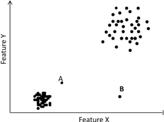
Figure 2.2: The Mahalanobis distance function can detect better outliers: When using Euclidean distance, the distance between data point B and the closest cluster centroid will be smaller than A and its cluster centroid; while data point ‘B’ is more obviously an outlier than data point ‘A’, because it does not follow the direction of the correlation of its cluster.
1: Cluster-Based methods These methods score outliers based on whether they belong to any predefined cluster and also the distance of the data points from clusters. There-fore, the performance of these methods has a high correlation with the efficiency of the clustering algorithm that they use [3]. Outliers that are chosen based on their comple-mentary membership to a cluster are often weak outliers or noise and not necessarily interesting to analyze. For example, a data point that is located at the margin of a large cluster is very different from a point that is completely away from all other clus-ters. Further, all data points in a small cluster may sometimes actually be outliers [3]. Therefore, a measure is needed to quantify the degree of abnormality of data points. Many cluster-based methods try to assign a score to the outliers, mostly by a simple definition as the distance of data points to cluster centroids. As clusters may have different shapes, Mahalanobis Distance is the best way to compute the distance that scales the square distances by the cluster variances along the different directions of correlation and it is used for effective statistical normalization. In other words, large distances in clusters with high variance may not be statistically significant within that data locality. It is possible that a data point that is closer to one of the clusters has a higher Mahalanobis distance than a data point which is far away on the basis of
Euclidean distance. In Figure 2.2 data point ‘B’ is more obviously an outlier than data point ‘A’.
Mahalanobis distance can be used as distance measure in many clustering algorithms, such as k-means algorithm [92, 16].
One advantage of cluster-based outlier detection methods is that they are based on global analysis of the data and small groups that do not fit within the major patterns can be easily detected using cluster-based methods.
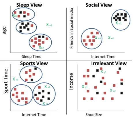
Mulleret al. propose a novel outlier scoring concept based on subspace clustering [61]. Their hypothesis is that regular objects show clustered behaviour in multiple subspaces even if the subspaces are very dissimilar to each other. On the other hand, outliers are clustered in some subspaces but deviate from these clusters if one considers other subspaces. Figure 2.3 shows that object o2 is clustered in two views, but not in the social view. Although there is a very similar clustering structure of the black objects in the “Sports View”, we see that this object deviates from its common grouping. Their outlier score,outrank, takes the similarity of subspaces into account and computes the outlierness degree based on the information available from subspace analysis. They rely on the general assumption that outliers are objects that do not agree with other data in at least a few of the attributes:
1. Outliers may be regular in some subspaces 2. They deviate in at least some subspaces.
They provide an abstract definition of a scoring function, given a subspace clustering as follows: let SCR= (C1, S1), ...,(Ck, Sk) be a subspace clustering, a set of clusters
Ci in their associated subspacesSi. A scoring function on SCR is then defined as:
score(o) = X
{C,S)∈SCR|o∈C}
evidence(o,(C, S), SCR) (2.2)
whereevidencecomputes a value of regularity forobeing clustered in subspace cluster (C, S) given the entire subspace clustering resultSCR. In their paper, they introduce three instantiations for the evidence function of equation 2.2.
Sleep View
Social View
Sports View
Irrelevant View
ag
e
Sport Ti
me
In
come
Fr ien d s in S ocial me d iaSleep Time Internet Time
Internet Time Shoe Size
Xo3 X o1 Xo2
X o1 X o2 X o3 X o1 X o2 X o3 X o3 X o1 X o2
the distance of a data point and other data points in the dataset (or k-nearest neigh-bour of each point) and the most isolated data points are considered as outliers. However, they suffer from computational growth. The complexity of computation is a function of the dimensionality of the data (m) and the number of records(n). There-fore, methods such as k-nearest-neighbours withO(n2m) runtime are not feasible for high-dimensionality datasets.
However, many approaches have been proposed in order to optimizek-nearest-neighbours and to produce a ranked list of potential outliers in a less complex way. Ramaswamyet al.[72] introduced a technique for speeding thek-nearest-neighbours algorithm. They partitioned the data into cells and only considered a cell and its directly adjacent neighbours. If that cell contains more than kpoints then the cell is located in a dense area and it is not likely to contain any outlier. By using this efficient indexing structure with linear running time, they improved the running speed of k-nearest-neighbours.
3: Density-based methods Local density is defined as the number of other points within a specified region of a data point. The difference between clustering and density-based methods is that clustering methods partition data points, while density-based methods partition data space [3]. Figure 2.4 illustrates the cases that cannot be discovered
A B Feature X Fea tu re Y
Figure 2.4: Impact of local density on outliers. If the threshold of a chosen distance-based methods is larger than the distance of A and the cluster centroid then the data point A will not be chosen as an outlier. If it is smaller then most of the points in the sparse cluster will be identified as outliers.
smaller distance threshold may result in incorrectly identifying many data points as outliers in the sparser clusters. It means that ranking returned by a distance-based method might be incorrect if there is significant heterogeneity in the local distribution of data.
The most popular density-based outlier methods are as follows:
• LOF: The Local Outlier Factor was originally presented in [12] as a measure to quantify the outlierness of the data points relative to regions of different densi-ties. Therefore, the score is defined based on local density instead of the nearest neighbour distance. In simple words, LOF compares the density of area around an object to the densities of the areas of the surrounding objects. However,LOF defines density as the inverse of the average of the smoothed reach-ability dis-tances in a neighbourhood; this definition is not the precise definition of density in terms of the number of data points within a specific region. Furthermore,LOF is only sensitive to the density of the area and ignores the orientation and the shape of the area [40]. Figure 2.5 shows the basic idea ofLOF.
A
Figure 2.5: Point A has a high LOF score because its density is lower than its neighbours densities. Dotted circles show the distance to each point’s third nearest neighbour.
• LOCI: Local Correlation Integral is a density-based method that uses the precise definition of density M(¯x, ) of a data point ¯x in terms of the number of data points within a predefined radius epsilon around a point. In other aspects, this method is similar to LOF in terms of using the local relations while defining the score of a data point [64].
The difference between proximity-based methods is the way proximity is defined. How-ever, the main difference between distance-based and the other two methods is the level of granularity of analysis [3]. In particular, clustering and density-based methods abstract the data by different forms of summarization; in order to compute the outlier score, only the distance of a point from its cluster centroid or the points in its local density area is computed. On the other hand, a distance-based algorithm with full granularity computes the distance of a point from all other points in the dataset. In clustering and density-based methods, the partitioning of the points and space is predefined and data points are compared with these predefined aggregations. This makes distance-based methods more fit to distinguish between noise and anomalies because the noisy data points will be included in the distance evaluations, rather than the cluster centroids. However, it is possible to modify cluster-based approaches to include the effects of noise. When it is done, the two approaches have very similar schemes.
2.2
Methods for Structured Data with Propositional Approach
The data used in this type of method is structured and the idea is to extract structured features and employ those features in a propositional outlier detection.
2.2.1 Feature-based Methods
Feature-based Methods use the graph representation of data to extract graph-centric features for outlier detection. An example of this type is a technique called ODDBALL, introduced by Akoglu et al. [5]. In this work they define an egonet as the immediate neighbourhood around a node, in other words, an egonet is the induced 1-step sub-graph for each node as shown in Figure 2.6. They extract egonet-based features to discover patterns from the graph structure in order to define normality. Outliers are the nodes that deviate from those patterns.
ego
ego -net
Figure 2.6: ego and ego-net in a toy graph.
2.3
Outlier Detection Methods for Relational Data with
non-propositional Approach
In the previous section, we explored a few of the many outlier detection methods that are designed for “flat” data. However, many real-world datasets have some sort of a structure. For example, social network data consists of individuals of different types where each indi-vidual is characterized by various sets of attributes. There are many applications of outlier detection that have a structured characteristic where the data consist of several interrelated data types. Therefore, instead of looking for individuals with values that deviate from spe-cific variables, the focus is to find individuals with deviating structures. This section focuses on methods that have been designed for relational data.
2.3.1 Supervised
The main idea in these methods is to use the structure of the data to assign objects to normal and abnormal classes. In the following we review a few examples of this type of methods.
Relational Classifier
By extending Markov networks to the relational setting, Taskar et al. drive a conditional distribution over the labels of all the individuals given the relational structure and the content attributes [89]. By using the conditional likelihood of the labels given the features they were able to improve the classification accuracy compared to the baseline methods.
Rule-Based Classifiers
Rule-based outlier detection methods extract rules that define the normal behaviour of the general population. At a given level of support and confidence, a test instance not consistent with any of the rules is identified as an outlier. An associated confidence is assigned to each rule which is proportional to the ratio between the number of correctly classified training instances and the total number of training instances. Decision Trees are commonly used for rule learning [24].
Mahoney et al. try to overcome the common problem of intrusion detection techniques: the inability to detect novel attacks. They use an adaptive statistical data compression technique based on context modeling and prediction to model normal behavior from attack-free network traffic [56] and extract a set of attributes for each event. They then induce a set of conditional rules that have a very low probability of being violated, according to a model learned from normal traffic in the training data.
2.3.2 Unsupervised
Maervoetet al. applied a relational frequent pattern miner to automatically discover a set of rules from data; exceptions from these rules are considered potential outliers and are passed to the next step for human expert evaluation [55]. They built a tool to look for regularities in geographical data using the WARMR algorithm [20]. WARMR is based on a breath-first search of the pattern space and searches the space beginning from the most general patterns. First, it searches for rules that describe the regularities and all violations are defined as outliers.
There is other research that employs rule mining to identify outliers. The ruleX →Y holds in the transaction setDwithconfidence c% ifc% of transactions inDthat containX also contain Y. The rule X →Y has support of s% in transaction setD, if s% of transactions inDcontain X∪Y.
Based on the way they use the identified rules they can be categorized as follows:
• Rules with minimum support, minimum confidence : Agrawal et al. find all sets of items (itemsets) that have the support above minimum support. They refer to itemsets with minimum support as large itemsets. Then, they use the large itemsets to generate the desired rules. For every large itemset l, they find all non-empty subsets
of l. For every such subset a, output a rule of the form a ⇒ (l−a) if the ratio of support(l) to support(a) is at least minconf. Therefore, in order to generate the rules that have low support minsup must be set very low, this increases the running time of the algorithm and generates a lot of redundant rules [4].
• Rules with low support but high confidence [47] define sporadic rules to be the ones with low support and high confidence to find a rare, but strong association. For example, a rare association of two symptoms indicating a rare fatal disease. In order to do so they adopt an Apriori-Inverse approach which is similar to the Apriori algorithm and is based on a level-wise search. However, they invert the downward-closure principle of the Apriori algorithm and instead of all subsets of rules being over minsup and return all subsets that are under maxup.
• Exception rule mining: There are many of methods to extract exceptional rules from data. Suzuki et al., propose a method to discover a set of interesting rule pairs from a dataset [88]. Hussainet al. define interestingness with respect to already mined rules and evaluate a rule’s interestingness with respect to its support and confidence. Similar to [4], this work has an efficiency problem due to the low support[38].
Outlier Detection in ILP
Inductive Logic Programming is an important field at the intersection of machine learning and logic programming. Its goal is to induce relational descriptions of data in the form of logic programs. ILP has been used for relational outlier detection. One approach views an example as anomalous if it is not covered by a learned set of rules [10]. It logically harmonizes the background theory with the observations at hand and the main interest is singling out the set of observations that do not behave as predicted from the background knowledge. Their definition of the outlier is based on a set of observations rather than a single observation. They defined outliers as given a set ofPrlsrules that encode the general knowledge about the world and a set Pobs of facts encoding some observed aspects of the current status of the world. The structure P is defined as P =< Prls, Pobs >. A set of
O of observations is anomalous according to the general theory Prls and the other facts in
Pobs\O.
Another work measures the difference in generality between a rule set learned with the anomalous examples and a rule set learned without [9]. Intuitively, if a subset of examples
does not comply with a background theory and the whole set of examples, then this means that the hypothesis induced in the absence of this subset is significantly more general than the hypothesis induced when the examples are seen. Given a subset of examples O of ε, they argue that the compliance of these examples withε∪β and ¯ε∪β can be exploited in order to understand if the setO contains abnormal observation.
Community-based methods
Community-based methods are based on finding well-connected groups of individuals. Out-liers are the individuals that do not clearly belong to any community. Sun et al. use proximity of nodes in the graph to detect anomalies in bipartite graphs. They define out-liers as “bridge” nodes and edges that do not fit into any community. They first find the community of a node, also referred to as the “neighbourhood” of a node, by using the random-walk-with-restart Personalized PageRank (PPR) score. The neighbourhood of the given node consists of nodes with high PPR scores and then they define a metric to quantify the level of a given node to be a bridge node [86].
Gao et al. proposed a probabilistic model to interpret normal objects and outliers where the object information is described by some generative mixture model. They use k
components to describe the normal behaviour and one component for outliers. Community components are assumed to be drawn from Gaussian or multinomial distribution, while the distribution for the outlier component is uniform [29].
Muller et al. developed an outlier detection technique called GOutRank for heteroge-neous databases and attributed graphs [62]. Their main insight is that complex anomalies could be revealed in a subset of relevant attributes. Their previous work, OutRank, focused on high dimensional data and did not take into account graph substructure in assigning outlierness scores to the nodes. However, GOutRank extracts the hidden potential of graph clustering and detects complex outliers which deviate only with respect to a local sub-graph and subset of relevant attributes.
2.4
Outlier Detection Methods for Other Types of
Struc-tured Data
Multi-dimensional OLAP
The multi-dimensional data model defines numeric measures for a set of dimensions. A seminal approach to explore a multi-dimensional data-cube was presented by Sarawagi et al. They perform an analyst’s search for anomalies guided by pre-computed indicators of exceptions at various levels of detail in the cubes [79]. This enables users to notice abnormal patterns in the data at any level of aggregation. They annotate every cell in all possible aggregations of a data cube with a value that shows the degree of surprise that the quantity in the cell holds. They define a different degree of surprise with respect to the position of the cells and find exceptions at all levels of aggregation.
Attribute Outlier
Kohet al. introduce the notion of correlated subspaces that leverage the hierarchical struc-ture of XML to derive groups of attributes that are logically correlated in XML [46]. In order to define the extent of outlierness of a target attribute, they define two correlation-based outlier metrics. One metric quantifies the co-occurrence of a target attribute relative to its neighbours and the co-occurrence of its neighbours in its absence. The lower the value of this metric is, the higher the degree of outlierness will be. The other metric measures the conditional probability: given the neighbours of a target attribute the probability that the target value is introduced in the dataset is computed. Depending on the metric specification of users, the outlier score is computed based on the first or second metric.
2.5
Limitations of Current Outlier Detection Methods
Parametric models assume a specific distribution of the data and then learn the parameters to fit the data. Most of the time one of two scenarios occurs: The assumed generative model is too restrictive and the data do not fit the model well, therefore, many data points will be reported as outliers. The second scenario occurs when the model is too complex and the number of parameters is large. This case often results in overfitting the data. Parametric methods are not efficient when datasets are large since these methods use the
iterative EM algorithm that scans the entire data in each iteration of E (expectation ) and M (maximization) steps.
Most of the parametric methods lack interpretability, however, this issue may not be a problem for all parametric methods. For example, a simple version of Gaussian model may be described simply and intuitively in terms of features of the original data. Most proximity-based methods use distance to define outliers. Methods that summarize the data will not perform well in identifying true anomalies from noisy regions with low density. These methods need to combine global and local analysis in order to find the true outliers. In proximity-based methods particularly, the higher level of granularity results in greater accuracy. However increasing the granularity causes curse of dimensionality and makes the algorithm inefficient (in the worst case distance-based methods with full granularity can require Ω(N2) in a dataset with N records). Indexing can be used in order to prune the search for the outliers but it cannot be very effective when data is sparse. Another limitation of these methods is the quality of the outlier detection in high dimensional data where all points become almost equidistant from one another and contrast in distance is lost [36].
Background, Data Model and
Statistical Models
In this chapter we first provide an introduction to the object-relational data model, which is one of the main data models for structured data and is used to represent our data throughout this dissertation. In section 3.3 we discuss three synthetic and two real-world datasets that have been designed to evaluate the performance of our outlier detection methods. In section 3.5 we review the necessary background on statistical models that are employed in this dissertation. Section 3.6 explains the evaluation techniques we have utilized to examine the outlier detection methods that will be introduced in chapter 4 and 5.
3.1
Notation and Definition
We adopt a term-based notation for combining logical and statistical concepts [69, 45]. A functor is a function or a predicate symbol. Each functor has a set of values (constants) called the domain of the functor. The domain of a predicate is {T,F}. Predicates are usually written with uppercase Roman letters, other terms with lowercase letters. A predicate of arity at least two is arelationshipfunctor. Relationship functors specify which objects are linked. Other functors representfeaturesorattributesof an object or a tuple of objects (i.e., of a relationship). Apopulation is a set of objects. Aterm is of the form
f(τ1, . . . , τk) wheref is a functor and eachτi is a first-order variable or a constant denoting an object. A term/literal/formula isgroundif it contains no first-order variables, otherwise
Table 3.1: Notation and Definition Symbol Definition
a, b, a1, b1, . . . Constant
A, B,T,M, . . . First-order variable f, g, . . . , Functor, function symbol f(A, . . . , Ak) First-order term
f(A=a1, . . . , Ak=ak) Ground term
D Relational database
DC Database for the entire class of objects
Do Restriction of the input database to the target object f(A, ..., B) A parametrized random variable
V A set of first-order random variable
V =v Joint assignment of values to a set of PRVs
P(V =v)≡P(v) Joint probability that each variablefi takes on valuevi #D(V =v) Count of groundings that satisfy the assignment
A\v Ground a first-order variable
PD(V =v) Grounding count divided by the number of all possible groundings
B A Bayesian network structure
BC A Bayesian network structure learned withDC as the input database
θC Parameters learned forBC using Dc as the input database
θo Parameters learned forBC using Do as the input database φ A Formula generated by MLN
w Weight of a formula
pai Parent of nodei
it is a first-order term. In the context of a statistical model, we refer to first-order terms as
Parametrized Random Variables(PRVs) [45]. A grounding replaces each first-order variable in a term/literal/formula by a constant, the result is a ground term. A grounding may be applied simultaneously to a set of terms. A relational databaseDspecifies the values of all ground terms.
Consider a joint assignment (also known as conjunctive formula or conjunction in logic)
P(V = v) of values to a set of PRVs V . The grounding space of the PRVs is the set of all possible grounding, each applied to all PRVs in V. The count of groundings that satisfy the assignment with respect to a database D is denoted by #D(V = v). The
database frequency PD(V = v) is the grounding count divided by the number of all
Example The Opta dataset represents information about Premier League data (Sec. 3.4). The basic populations are teams, players, and matches with corresponding first-order vari-ablesT,P,M. As shown in Table 3.2, the groundings count can be visualized in terms of a groundings table [82], also called a universal schema [77]. The first three column headers show first-order variables ranging over different populations. The remaining columns repre-sent terms. Each row reprerepre-sents a single grounding and the values of the ground terms are defined by the grounding. In terms of the grounding table, the grounding count of a joint assignment is the number of rows that satisfy the conditions in the joint assignment. In the network view representation of data, a grounding count is the number of subgraphs that satisfy a given conjunction as shown in Figure 3.2. The database frequency is the grounding count divided by the total number of rows in the groundings table. Counts are based on the 2011-2012 Premier League Season. We count only groundings (team,match) such that team plays in match. Each team, including Wigan Athletics, appears in 38 matches. The total number of team-match pairs is 38×20 = 760.
Example Figure 3.1 shows an example database. The ground literal
(ShotEff(P,M) =Low){P\123, M\1}= (ShotEff(123,1) =Low) evaluates to true in this database. For the grounding count we have
#D(ShotEff(P,M) =Low){P\123}) = 2.
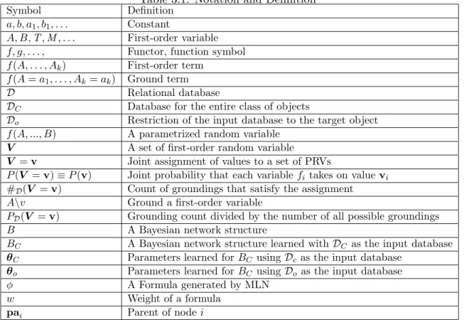
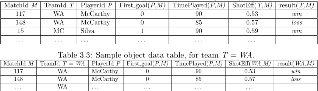
Table 3.2: Sample population data table (Soccer).
MatchIdM TeamIdT PlayerIdP First goal(P,M) TimePlayed(P,M) ShotEff(T,M) result(T,M)
117 WA McCarthy 0 90 0.53 win
148 WA McCarthy 0 85 0.57 loss
15 MC Silva 1 90 0.59 win
. . . .
Table 3.3: Sample object data table, for teamT =WA.
MatchIdM TeamIdT=WA PlayerIdP First goal(P,M) TimePlayed(P,M) ShotEff(WA,M) result(WA,M)
117 WA McCarthy 0 90 0.53 win
148 WA McCarthy 0 85 0.57 loss
. . . WA . . . .
3.2
Object-relational Data Model
Player ID 112 232 123
PlayeID MatchID ShotEff(P,M) TackleEff(P,M)
112 1 Med. High 112 2 High High 123 1 Low Low 123 2 Low Med Player Team AppearsPlayerInMatch Team ID 1 12 20 Match Match ID 1 2 4
TeamID MatchID ShotEff(T.M) TackleEff(T,M)
20 1 Med. Med.
20 2 Med. Med.
1 1 Low Low
1 2 Low Med
AppearsTeamInMatch
Figure 3.1: An example database
Table 3.4: Example of grounding count and frequency in the Premier League, for the con-junctionpassEff(T,M) =high∧shotEff(T,M) =high∧Result(T,M) =win.
Database
Count or #
D(
V
=
v
)
Frequency or
P
D(
V
=
v
)
Population
76
76
/
760 = 0
.
10
Wigan Athletics
7
7
/
38 = 0
.
18
Table 3.5: Instances of the conjunction: passEff(T,M) =high∧ shotEff(T,M) =high∧
Result(T,M) =win in the network representation of Figure 3.2.
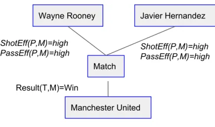
Team Player MatchID shotEff(T,M) passEff(T,M) Result(T,M) Manchester United Javier Hernandez 119 high high win Manchester United Anderson 119 high high win
Match Player ShotEff(P,M) PassEff(P,M) Result(T,M) Team Wayne Rooney Match Javier Hernandez ShotEff(P,M)=high
PassEff(P,M)=high ShotEff(P,M)=highPassEff(P,M)=high
Result(T,M)=Win
Manchester United
Figure 3.2: Example of two instances of conjunction: passEff(T,M) =hi, shotEff(T,M) =hi, Result(T,M) =win, in the network representation. We use the con-junctions to define subgraphs.
1. Object Identity. Each object has a unique identifier that is the same across contexts. For example, a player has a name that identifies him in different matches.
2. Class Membership. An object is an instance of a class, which is a collection of similar objects. Objects in the same class share a set of attributes. For example, van Persie is a player object that belongs to the class striker, which is a subclass of the class player. 3. Object Relationship. Objects are linked to other objects. Both objects and their links have attributes. A common type of object relationship is a component relationship between a complex object and its parts.
For example, a match links two teams, and each team comprises a set of players for that match. A difference between relational and vectorial data is that an individual object is characterized not only by a list of attributes but also by its links and by attributes of the object linked to it. We refer to the substructure comprising this information as theobject data. Object-relational data can be represented as a network as shown in Figure 3.2.
Example A query for computing object data for the soccer team Arsenal includes the selection conditionT eamID =Arsenal. Note that object data features all the data of the object as well as the data from more complex objects within that object.
The appropriateobject data tableis formed from the population data table by restrict-ing the relevant first-order variable to the target object. For example, the object database for target TeamWiganAthleticforms a subtable of the data table of Table 3.2 that contains only rows where TeamID =WA; see Table 3.3. In database terminology, an object database is like a view centered on the object.
3.3
Synthetic Datasets
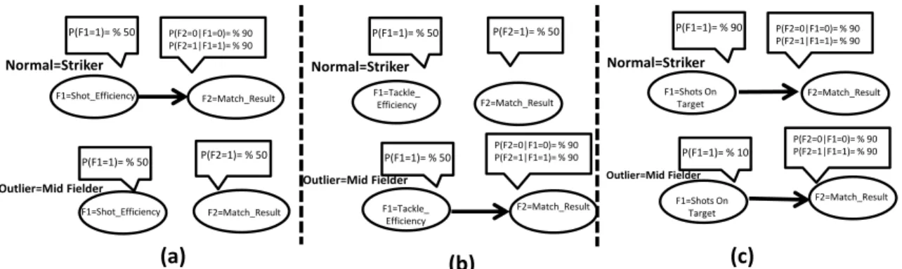
The main goal of designing synthetic experiments is to test the methods on easy to detect outliers. We generated three synthetic datasets with normal and outlier players using the distributions represented in the three Bayesian networks of Figure 3.3. Each player partic-ipates in 38 matches, similar to the real-world data. Each match assigns a value to each featureFi, i= 1,2 for each player.
These datasets are as follows:
High Correlation Normal individuals exhibit a strong association between their fea-tures, outliers have no association. Both normals and outliers have a close to uniform distribution over single features. See Figure 3.3(a).
Low Correlation Normal individuals exhibit no association between their features, out-liers have a strong association. Both normals and outout-liers have a close to uniform distribution over single features. See Figure 3.3(b).
Single featuresBoth normal and outlier individuals exhibit a strong association between their features. In normals, 90% of the time feature 1 has value 0. For outliers, feature 1 has value 0 only 10% of the time. See Figure 3.3(c).
We used the mlbench package inR to generate synthetic features in matches and followed these distributions for 240 normal players and 40 outliers. We followed the real-world Opta data in terms of number of normal and outlier individuals.
3.4
Real-world Datasets
In this dissertation, real world data tables are prepared from Opta data [57] and IMDb [39].Table 3.6 lists the populations and features. Table 3.7 shows summary statistics for the datasets.
F1=Shot_Efficiency F2=Match_Result P(F1=1)= % 50 P(F2=0|F1=0)= % 90 P(F2=1|F1=1)= % 90 Normal=Striker P(F1=1)= % 50 P(F2=1)= % 50 Outlier=Mid Fielder P(F1=1)= % 50 P(F1=1)= % 50 P(F1=1)= % 90 P(F2=0|F1=0)= % 90 P(F2=1|F1=1)= % 90 P(F1=1)= % 10 (a) (b) (c) P(F2=1)= % 50 P(F2=0|F1=0)= % 90 P(F2=1|F1=1)= % 90 P(F2=0|F1=0)= % 90 P(F2=1|F1=1)= % 90 F1=Shot_Efficiency F2=Match_Result Normal=Striker F1=Tackle_ Efficiency F2=Match_Result F1=Tackle_ Efficiency F2=Match_Result Normal=Striker F1=Shots On Target F2=Match_Result F1=Shots On Target F2=Match_Result
Outlier=Mid Fielder Outlier=Mid Fielder
Figure 3.3: Illustrative Bayesian networks. The networks are not learned from data, but hand-constructed to be plausible for the soccer domain. (a) High Correlation; (b) Low Correlation; (c) Single Attributes.
Individuals Features Soccer-Player
per Match TimePlayed,Goals,SavesMade, ShotEff,PassEff,WinningGoal, FirstGoal,PositionID,
TackleEff,DribbleEff, ShotsOnTarget
Soccer-Team
per Match ResultP ,TeamFormation,
Goals,µShotEff,µPassEff,
µTackleEff,µDribbleEff. IMDb-Actor Quality, Gender
IMDb-Director Quality,avgRevenue
IMDb-Movie year,isEnglish,Genre,Country, RunningTime, Rating by User
IMDb-User Gender, Occupation.
Premier League Statistics
IMDb Statistics
Number Teams
20
Number Movies
3060
Number Players
484
Number Directors
220
Number Matches
380
Number Actors
98690
avg player per match
26.01
avg actor per movie
36.42
Table 3.7: Summary statistics for the IMDb and the Premier League datasets
Soccer Data The Opta data were released by Manchester City. It lists all the ball actions within each game, by each player, for the 2011-2012 season. Number of goals, passes, fouls, tackles, saves and blocks, and also the position assigned to a player in a match, are examples of the information associated with each player. For each player in a match, our dataset contains eleven player features. For each team in a match, there are five features computed as player feature aggregates, as well as the team formation and the result (win, tie, loss). There are two relationships,Appears Player(P,M),Appears Team(T,M). We refer to the Premier League data as the Soccer dataset. Table 3.7 shows summary statistics for the datasets.
IMDb Data The Internet Movie Database (IMDb) is an on-line database of information related to films, television programs and video games. The IMDb website offers a dataset containing information on cast, crew, titles, technical details and biographies in a set of compressed text files. We preprocessed the data similar to Peralta et. al approach [67], to obtain a database with seven tables, one for each population and one for the three relationships: Rated(User,Movie), Directs(Director,Movie), andActsIn(Actor,Movie).
In real-world data there is no ground truth about which objects are outliers. To address this issue we employ a one-class design: we learn a model for the class distribution, with data from only that class. We then rank all individuals from the normal class, together with all objects from a contrast class treated as outliers, in order to test whether an outlier score recognizes objects from the contrast class as outliers. Table 3.8 shows the normal and contrast classes for three different datasets. In-class outliers are possible, e.g. unusual strikers are still members of the striker class. Chapter 5 describes a few in-class outliers. In the soccer data we considered only individuals who played more than 5 matches out of a maximum 38.