Yuan, Fajie (2018) Learning implicit recommenders from massive
unobserved feedback. PhD thesis.
https://theses.gla.ac.uk/30862/
Copyright and moral rights for this work are retained by the author
A copy can be downloaded for personal non-commercial research or study,
without prior permission or charge
This work cannot be reproduced or quoted extensively from without first
obtaining permission in writing from the author
The content must not be changed in any way or sold commercially in any
format or medium without the formal permission of the author
When referring to this work, full bibliographic details including the author,
title, awarding institution and date of the thesis must be given
Learning Implicit Recommenders
from Massive Unobserved Feedback
Fajie Yuan
School of Computing Science
College of Science and Engineering
University of Glasgow
This dissertation is submitted for the degree of
Doctor of Philosophy (PhD)
14
thSep 2018
I hereby declare that except where specific reference is made to the work of others, the contents of this dissertation are original and have not been submitted in whole or in part for consideration for any other degree or qualification in this, or any other University.
This dissertation is the result of my own work, under the supervision of Pro-fessor Joemon M. Jose and Dr. Simon Rogers.
Fajie Yuan Sep, 2018
Acknowledgements
First of all, I would like to express my sincere gratitude to my doctoral supervisor Prof. Joemon M. Jose. Without your careful instruction, I would never achieve so much success and finish the degree. Joemon is not only a nice and easy-going professor, but also one of the best friends in my life. Thanks for your support and encouragement. Thanks for believing in me and teaching me. With your supervision, I really enjoy my research and my Ph.D life.
Second, I would like to show my great respect to my second supervisor Dr. Simon Rogers. Thanks for agreeing to be my second supervisor. Simon is a cool guy and a helpful friend. Thanks for giving me so much good advice in my annual review.
Third, I want to thank Dr. Guibing Guo, Dr. Weinan Zhang and Dr. Xiang-nan He, who I have worked with for many years. They are the most outstanding young researchers in my field. I have learned a lot from him during collaboration and got many help from them. Without their help, I will not have so many good work accepted by prestigious conferences.
Fourth, I would like to thank my internship advisor Dr. Alexandros Karat-zoglou and Ioannis Arapakis in Telefonica Research. Alexandros and Ioannis are great researchers in industry and gave me so much invaluable advice in guiding me towards doing useful and successful research.
Fifth, I would like to thank my two examiners Prof. Pablo Castells and Dr. Ke Yuan for their expert advice to further improve my thesis.
Sixth, I would like to thank my university colleagues: Stewart, Rami, Philip, James, Jesus, Fatma, Jarana, David Maxwell, Jorge Paule, Stuart Mackie, Yashar Moshfeghi, Nujud and Xin Xin. Particularly, thanks Stewart for many help on my research.
Ya-Last but not least, I would like to acknowledge the most important people in my life — my parents and my wife. I want to give my best thanks to them for their love and unconditional supports during these years!
Abstract
Recommender systems have become an attractive research topic during the last two decades, and are utilized in a broad range of areas, including movies, music, images, advertisements, natural language, search engines, and social websites, etc. Early recommendation research largely focused on explicit feedback such as user ratings. However, in practice most observed user feedback is not explicit but implicit, such as clicks, purchases and dwell time, where users’ explicit pref-erence on items is not provided. Moreover, implicit feedback is usually tracked automatically and, thus, it is more prevalent, inexpensive and scalable.
In this thesis we investigate implicit feedback techniques for real-world recom-mender systems. However, learning a recomrecom-mender system from implicit feedback is very challenging, primarily due to the lack of negative feedback. While a com-mon strategy is to treat the unobserved feedback (i.e., missing data) as a source of negative signal, the technical difficulties cannot be overlooked: (1) the ratio of positive to negative feedback in practice is highly imbalanced, and (2) learning through all unobserved feedback (which easily scales to billion level or higher) is computationally expensive.
To effectively and efficiently learn recommender models from implicit feed-back, two types of methods are presented, that is, negative sampling based stochastic gradient descent (NS-SGD) and whole sample based batch gradient descent (WS-BGD). Regarding the NS-SGD method, how to effectively sample informative negative examples to improve recommendation algorithms is inves-tigated. More specifically, three learning models called Lambda Factorization Machines (lambdaFM), Boosting Factorization Machines (BoostFM) and Geo-graphical Bayesian Personalized Ranking (GeoBPR) are described. While regard-ing the WS-BGD method, how to efficiently use all unobserved implicit feedback data rather than resorting to negative sampling is studied. A fast BGD learning
The last research work is on the session-based item recommendation, which is also an implicit feedback scenario. However, different from above four works based on shallow embedding models, we apply deep learning based sequence-to-sequence model to directly generate the probability distribution of next item. The proposed generative model can be applied to various sequential recommendation scenarios.
To support the main arguments, extensive experiments are carried out based on real-world recommendation datasets. The proposed recommendation algo-rithms have achieved significant improvements in contrast with strong bench-mark models. Moreover, these models can also serve as generic solutions and solid baselines for future implicit recommendation problems.
Table of Contents
Declaration i
Acknowledgements ii
Abstract iv
Table of Contents vi
List of Figures xii
List of Tables xvi
I
Introduction and Background
1
1 Introduction 2
1.1 Background on Recommendation . . . 2
1.2 Implicit Feedback Recommendation . . . 4
1.3 Thesis Statement . . . 6
1.4 Thesis Structures and Contributions . . . 8
1.5 Related Publications . . . 9
2 Background of Implicit Recommendation 11 2.1 Overview on Recommender Systems . . . 11
2.1.1 Goals and Formulation of Recommender Systems . . . 11
2.1.2 Types of Recommender Systems . . . 14
2.1.2.1 Collaborative Filtering Based Recommendations . 15 2.1.2.2 Content/Context-Based Recommendations . . . . 16
2.2 Overview on Implicit Recommendation . . . 18
2.3 Implicit Feedback Model Overview . . . 22
2.3.1 Factorization Models . . . 22
2.3.1.2 SVD++ (Koren and Bell, 2015) . . . 24
2.3.1.3 SVDFeature (Chen et al., 2012) . . . 24
2.3.1.4 Factorization Machines (Rendle,2010) . . . 25
2.3.1.5 Tucker Decomposition (Tucker,1966) . . . 26
2.3.2 Deep Learning Models . . . 27
2.3.2.1 Neural Collaborative Filtering (He et al.,2017) . 27 2.3.2.2 Neural Factorization Machines (He and Chua,2017) 28 2.3.3 Objective Functions with Negative Sampling . . . 29
2.3.3.1 Pointwise Loss with Negative Sampling . . . 30
2.3.3.2 Pairwise Loss with Negative Sampling . . . 31
2.4 Evaluation of Implicit Recommendation . . . 32
2.4.1 Implicit Feedback Datasets . . . 32
2.4.2 Evaluation Protocols . . . 33
2.4.3 Evaluation Metrics . . . 34
II
SGD with Negative Sampling
37
3 Lambda Factorization Machines 38 3.1 Introduction . . . 393.2 Related Work . . . 40
3.2.1 Content/Context-based Recommender Systems . . . 40
3.2.2 Learning-to-Rank . . . 41
3.3 Preliminaries . . . 43
3.3.1 Pairwise Ranking Factorization Machines . . . 43
3.3.2 Lambda Motivation . . . 44
3.4 Lambda Strategies . . . 47
3.4.1 Static and Context-independent Sampler . . . 48
3.4.2 Dynamic and Context-aware Sampler . . . 50
3.4.3 Rank-aware Weighted Approximation . . . 51
3.5 Lambda with Alternative Losses . . . 55
3.6 Experiments . . . 56
3.6.1 Experimental Setup . . . 56
TABLE OF CONTENTS 3.6.1.2 Evaluation Metrics . . . 57 3.6.1.3 Baseline Methods . . . 58 3.6.1.4 Hyper-parameter Settings . . . 58 3.6.2 Performance Evaluation . . . 59 3.6.2.1 Accuracy Summary . . . 59
3.6.2.2 Effect of Lambda Surrogates/Samplers . . . 61
3.6.2.3 Effect of Adding Features . . . 62
3.6.2.4 Lambda with Alternative Loss Functions . . . 63
3.7 Chapter Summary . . . 64
4 Boosting Factorization Machines 66 4.1 Introduction . . . 66
4.2 Related Work about Boosting . . . 68
4.3 Preliminaries . . . 69
4.4 Boosted Factorization Machines . . . 70
4.4.1 BoostFM . . . 70
4.4.2 Component Recommender . . . 73
4.4.2.1 Weighted Pairwise Factorization Machines . . . . 73
4.4.2.2 Weighted LambdaFM Factorization Machines . . 74
4.5 Experiments . . . 75 4.5.1 Experimental Setup . . . 75 4.5.1.1 Datasets . . . 75 4.5.1.2 Evaluation Metrics . . . 76 4.5.1.3 Baseline Methods . . . 76 4.5.1.4 Hyper-parameter Settings . . . 77 4.5.2 Performance Evaluation . . . 78 4.5.2.1 Accuracy Summary . . . 78
4.5.2.2 Effect of Number of Component Recommenders . 78 4.5.2.3 Effect of Sampling Strategies (i.e., ρ) . . . 81
4.5.2.4 Effect of Adding Features . . . 82
4.6 Chapter Summary . . . 83
5 Geographical Bayesian Personalized Ranking 84 5.1 Introduction . . . 85
5.2 Related Work for POI recommendation . . . 86
5.3 Geo-spatial Preference Analysis . . . 88
5.3.1 Data Description . . . 88
5.3.2 Motivation . . . 89
5.3.3 Proximity Analysis . . . 90
5.4 Preliminaries . . . 91
5.4.1 Problem Statement . . . 91
5.4.2 BPR: Ranking with Implicit Feedback . . . 92
5.5 The GeoBPR Model . . . 93
5.5.1 Model Assumption . . . 93
5.5.2 Model Derivation . . . 95
5.5.3 Model Learning and Sampling . . . 98
5.6 Experiments . . . 99 5.6.1 Experimental Setup . . . 99 5.6.1.1 Baseline Methods . . . 99 5.6.1.2 Parameter Settings . . . 100 5.6.1.3 Evaluation Metrics . . . 101 5.6.2 Experimental Results . . . 101
5.6.2.1 Summary of Experimental Results . . . 101
5.6.2.2 Impact of Neighborhood . . . 103
5.6.2.3 Impact of Factorization Dimensions . . . 104
5.7 Chapter Summary . . . 104
III
Batch Gradient with All Samples
106
6 Fast Batch Gradient Descent 107 6.1 Introduction . . . 1086.2 Related Work . . . 109
6.3 Preliminaries . . . 111
6.3.1 The Generic Embedding Model . . . 111
6.3.2 Optimization with BGD . . . 112
6.3.3 Efficiency Challenge . . . 113
TABLE OF CONTENTS
6.4.1 Partition of the BGD Loss . . . 114
6.4.2 Constructing a Dot Product Structure . . . 115
6.4.3 Efficient Gradient . . . 116
6.4.4 Effective Weighting on Missing Data . . . 118
6.5 ImprovedfBGD . . . 120
6.5.1 Gradient Instability Issue in CF Settings . . . 120
6.5.2 Solving the Unstable Gradient Problem . . . 122
6.6 Experiments . . . 123
6.6.1 Experimental Settings . . . 123
6.6.1.1 Datasets . . . 123
6.6.1.2 Baselines and Evaluation Protocols . . . 124
6.6.1.3 Experimental Reproducibility . . . 125
6.6.2 Performance Evaluation . . . 126
6.6.2.1 Model Comparison . . . 126
6.6.2.2 Impact of fBGD Weighting . . . 129
6.6.2.3 Impact of Adding Features . . . 131
6.6.2.4 Efficiency . . . 132
6.7 Chapter Summary . . . 132
IV
Deep Learning for Session-based Recommendation
134
7 Deep Learning for Session-based recommendation 135 7.1 Introduction . . . 1367.2 Preliminaries . . . 138
7.2.1 Top-N Sequential Recommendation . . . 138
7.2.2 Limitations of Caser . . . 139
7.2.3 Related Work . . . 141
7.3 Model Design . . . 142
7.3.1 Sequential Generative Modeling . . . 142
7.3.2 Network Architecture . . . 144
7.3.2.1 Embedding Look-up . . . 144
7.3.2.2 Dilation . . . 144
7.3.3 Residual Learning . . . 145
7.3.3.1 Masking . . . 148
7.3.4 Final Layer, Network Training and Generating . . . 148
7.4 Experiments . . . 150
7.4.1 Datasets and Experiment Setup . . . 150
7.4.1.1 Datasets and Preprocessing . . . 150
7.4.1.2 Hyper-parameter Settings . . . 152
7.4.1.3 Evaluation Protocols . . . 153
7.4.2 Results Summary . . . 153
7.5 Chapter Summary . . . 156
V
Conclusion
157
8 Conclusions and Future Work 158 8.1 Contribution Summary . . . 1588.2 Future Work . . . 161
8.3 Closing Remarks . . . 163
List of Figures
1.1 Sparse matrices of implicit (a) and explicit (b) data. u and i
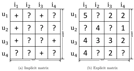
de-notes user and item, respectively. “+” and “?” denote positive (e.g., a click) and unobserved feedback (i.e., no click), respectively. The numerical values in (b) represent explicit rating scores that users assigned to items, while on (a), users’ explicit feedback (i.e., ratings) is not observed. . . 5
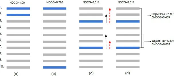
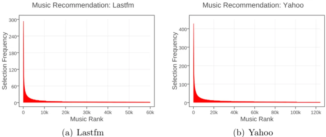
3.1 A set of items ordered under a given context (e.g., a user) using a binary relevance measure. The blue bars represent relevant items for the context, while the light gray bars are those not relevant. (a) is the ideal ranking; (b) is a ranking with eight pairwise errors; (c) and (d) are a ranking with seven pairwise errors by moving the top items of (b) down two rank levels, and the bottom preferred items up three. The two arrows (black solid and red dashed) of (c) denote two ways to minimize the pairwise errors. (d) shows the change in NDCG by swapping the orders of two items (e.g., item 7 and item 1). . . 46 3.2 Item popularity on the Lastfm (short for Last.fm) and Yahoo
datasets plotted in the linear scale. . . 48
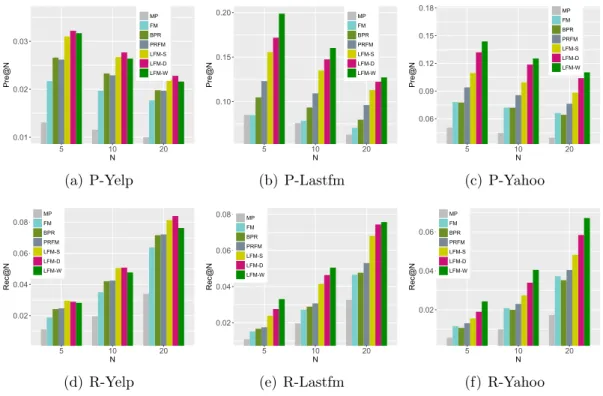
3.3 Performance comparison w.r.t. top-N values, i.e., Pre@N (P) and Rec@N (R). . . 60
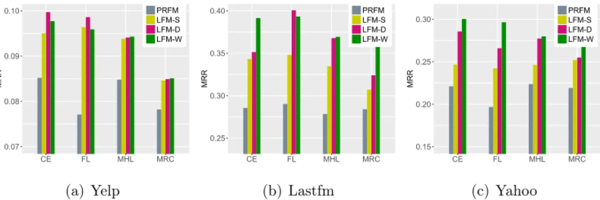
3.4 Parameter tuning w.r.t. MRR. . . 60
3.5 The variants of PRFM and LambdaFM based on various pairwise loss functions. . . 63
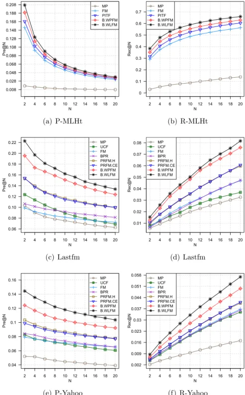
4.1 Performance comparison w.r.t., top-N values, i.e., Pre@N and Rec@N. N ranges from 2 to 20, the number of component recommender T
is fixed to 10, and ρ for B.WLFM is fixed to 0.3. . . 79
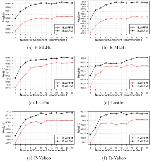
4.2 Performance trend of BoostFM (i.e., B.WPFM and B.WLFM) w.r.t. Pre@10 and Rec@10. T ranges from 1 to 50, and ρ is fixed
to 0.3. . . 80
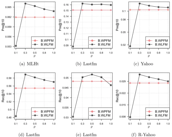
4.3 Performance trend of BoostFM by tuning ρ w.r.t. Pre@10 &
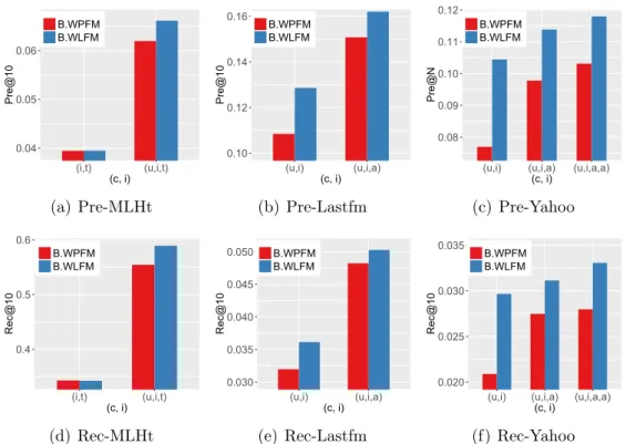
Rec@10. ρ ∈ {0.1,0.3,0.5,0.8,1.0},T = 10. . . 81 4.4 Performance comparison w.r.t. Pre@10 & Rec@10 with context
and side information. In (a) (d), (i, t) denotes an item-tag (i.e., movie-tag) pair and(u, i, t)denotes a user-item-tag triple; in (b)(c)(e)(f) (u, i)denotes a user-item (i.e., user-music) pair and(u, i, a)denotes a user-item-artist triple; similarly, (u, i, a, a) denotes a user-item-artist-album quad. T is fixed to 10, and ρ is fixed to 0.3. . . 82
5.1 The overview of a random user’s multi-center mobility behaviours on Phoenix and Las Vegas. . . 89
5.2 Two scenarios of user-POI pairs. . . 94
5.3 Performance comparison with respect to top-N values in terms of Pre@N and Rec@N. . . 102
5.4 Performance comparison with different µ. . . 102
5.5 Performance comparison with different k. . . 103
6.1 Impact of negative item sampling on SGD on the Last.fm data set. The x-axis is the number of sampled negative items for each positive one. Better accuracy (a) can be obtained by sampling more negative instances at the expense of longer training times (b). More details on the experimental settings are given in Section 6.6. 108
6.2 The structure of sparse input matrix and dense embedding matrix for user-fields. XU (left) denotes the user-field matrix with only
user IDs; XU (right) denotes the user-field matrix with both user
LIST OF FIGURES
6.3 Performance of the improved fBGD (Section 6.5.2) and standard
fBGD on Last.fm with four features. For the standardfBGD, some
gradients will be evaluated as infinite (NaN) when γ > 5×10⁻⁵. As can be seen, fBGD with vanishing gradient performs poorly on
Last.fm even by carefully tuning the learning rate. . . 120
6.4 Impact of weighting parameters α0 and ρ. . . 130 6.5 Training costs offBGD vs BGD. One unit in (a) and (b) represents
26 and 165 seconds respectively. . . 131
7.1 The core structure of Caser. The red, yellow and blue regions denotes a 2×k, 3×k and 4×k convolution filter respectively,
where k= 5. The purple row stands for the true next item. . . . 137 7.2 The proposed generative architecture with 1D standard CNNs (a)
and efficient dilated CNNs (b). An example of a standard 1D convolution filter and dilated filters are shown at the bottom of (a) and (b) respectively. The blue dash line is the identity map which exists only for residual block (b) in Fig.7.3. . . 140
7.3 Dilated residual blocks (a), (b) and one-dimensional transforma-tion (c). (c) shows the transformatransforma-tion from the 2D filter (C = 1)(left) to the 1D 2-dilated filter (C = 2k) (right); the vertical
black arrows represent the direction of the sliding convolution. In this work, the default stride for the dilated convolution is 1. Note the reshape operation in (b) is performed before each convolution in (a) and (b) (i.e.,1×1and masked1×3), which is then followed by a reshape back step after convolution. . . 146
7.4 The future item can only be determined by the past ones according to Eq. (7.1). (a) (d) and (e) show the correct convolution process, while (b) and (c) are wrong. E.g., in (d), items of {1,2,3,4} are
masked when predicting 1, which can be technically implemented by padding. . . 146
7.5 Convergence behaviors of MUSIC_L100. GRU is short for GRURec.
g = 256k means the number of training sequences (or sessions) of one unit in x-axis is 256k. Note that (1) to speed up the evaluation, all of the convergence tests are performed on the first 1024 sessions in the testing set, which also applies to Fig. 7.6; (2) clearly, GRU and Caser have not converged in above figures. . . 153
List of Tables
3.1 Basic statistics of datasets. Each entry indicates a context-item pair 57
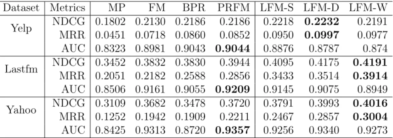
3.2 Performance comparison on NDCG, MRR and AUC. For each
mea-sure, the best result is indicated in bold. . . 57
4.1 Basic statistics of datasets. Each tuple represents an observed context-item interaction. Note that tags on the MLHt dataset are regarded as recommended items (i.e., i in xi), while a user-item (i.e., user-movie) pair is regarded as context (i.e., cinxc). . . 75
5.1 Basic statistics of Datasets. . . 88
5.2 Ratios of P0/P. . . 90
5.3 List of notations. . . 93
5.4 Performance comparison. PX and LV denotes Phoenix and Las Vegas respectively. GBPRa and GBPRb denote GeoBPR with assumption a and b respectively. . . 100
6.1 Basic statistics of the datasets. The density on Yahoo and Last.fm is 0.28% and 0.033% respectively. . . 126
6.2 Comparison of implicit embedding models. . . 126
6.3 Accuracy evaluation on Yahoo. fBGD− denotesfBGD with a uniform weight (ρ = 0). The training iterations of fBGD− is 400. For each measure, the best results for SGD and all models are indicated in bold, which also applies to Table 6.4. . . 127
6.5 Accuracy evaluation on Last.fm by adding features. u, p, i and a
denote user, last item (song), next item and artist respectively. Noteu &p belong to the user-field, andi &a belong to the
item-field. All hyper-parameters of fBGD are fixed. . . 129
7.1 Session statistics of all data sets. MUSIC_M5 denotes MUSIC_M with maximum session size of 5. The same applies to MUSIC_L. ‘M’ denotes 1 million. . . 148
7.2 Accuracy comparison. The upper, middle and below tables are MRR@5, HR@5and NDCG@5 respectively. . . 149 7.3 Accuracy comparison. The upper, middle and below tables are
MRR@20, HR@20and NDCG@20respectively. . . 151 7.4 Effects of sub-session in terms of MRR@5. The upper, middle and
below tables represent GRU, Caser and NextItNet respectively. “10”, “20”, “50” and “100” the session length. All high parameters are fixed. . . 152
7.5 Effects (MRR@5) of increasing embedding size. The upper and below tables are MUSIC_M5 and MUSIC_L100 respectively. . . 152
7.6 Effects of the residual block in terms of MRR@5. “Without” means no skip connection. “M5”, “L5”, “L10” and “L50” denote MUSIC_-M5 , MUSIC_L5 , MUSIC_L10 and MUSIC_L50 respectively. All high parameters are fixed. . . 154
Part I
Introduction and Background
The thesis focuses on the item recommendation task from implicit feedback. The main research question is how to ef-fectively use the large-scale unobserved feedback. This part includes Chapter 1 for introduction and Chapter 2 for im-plicit feedback model reviews. In Chapter1, we have surveyed the background information for implicit feedback based item recommendation, and then provided thesis motivations, state-ments, challenges and contributions. In Chapter2, we investi-gated the most widely used prediction models, objective func-tions and evaluation metrics for item recommendation from implicit feedback.
Introduction
1.1
Background on Recommendation
In the last two decades, the emerging growth of the Internet has brought a huge amount of digital information, including but not limited to, texts, images, au-dios/videos and electronic products. Meanwhile, a variety of social networks (e.g., Facebook1 and Weichat2 ), electronic business platforms (e.g., Amazon3),
and multimedia sharing websites (e.g., Youtube4) have become more and more
popular. The volume of online information is growing at an unbelievably fast rate, since a large number of visitors in these application platforms can frequently cre-ate, upload and share new information (Shi, 2013). With such huge amount of information, it is difficult for users to find useful items and make effective deci-sions, which is referred to as information overload5. To deal with this issue, two
important information processing technologies have been developed (Belkin and
Croft, 1992): information retrieval and recommendation.
In an information retrieval (IR) system, users explicitly present their infor-mation needs by sending a query to a search engine (e.g., Google6) (Costa and
Roda,2011;Belkin and Croft,1992). The system processes the request by
search-ing existsearch-ing resources and returns a list of matched items accordsearch-ing to a certain retrieval algorithm. On the contrary, in a recommendation platform, the sys-tem (e.g., Amazon) typically automatically generates recommendations based on
1 https://www.facebook.com/ 2 https://web.wechat.com/ 3 https://www.amazon.co.uk// 4 https://www.youtube.com 5 https://en.wikipedia.org/wiki/Information_overload 6 https://www.google.co.uk/
1.1 Background on Recommendation
users’ profiles rather than an explicit query. Both ways play an important role in obtaining knowledge from the Internet. The main difference lies in that the needs of a user in an IR system are expressed explicitly, whereas they are typically un-specified in a recommender system (RS), and as a result, the user is more likely to passively accept recommended information (Shi,2013). In addition, compared to search engines, recommender systems help users discover new unexpected items, or support serendipitous (Kawamae, 2010) discoveries, which they may not ini-tially realize when formulating the query (Tintarev et al., 2013; Shi, 2013). A good IR system typically needs to have accuracy guarantee in matched items, which, however, is not enough for a RS system. Recommendation accuracy, per-sonalization, and context are all important factors for evaluating a RS system. In this thesis, our main research focus is to study and develop new advancement in recommender systems, and address critical research challenges in this domain. A recommender system is formally defined as “a subclass of information fil-tering system that seeks to predict the ‘rating’ or ‘preference’ a user would give to
an item” (Ricci et al., 2011). Recommender systems are important in assisting
users with their choices. A good recommender system is supposed to suggest the right items to the right person in the right context. In recent years recommender systems have been widely used in a variety of domains (Sheth et al.,2010), such as recommending movies we might like (Katarya and Verma,2017), places we might visit (Yuan et al., 2016d), things we might buy (Yuan et al., 2018a), friends we may know (Yuan et al., 2016a) and queries we may type (Baeza-Yates et al.,
2004).
There are two types of recommender systems according to the way to gen-erate recommendations: collaborative filtering (Koren and Bell, 2015) and con-tent/context based recommendation (Rendle, 2012). Collaborative filtering (aka neighborhood-based) approaches build the recommendation model based on users’ past histories, or decisions made by other similar users (i.e., neighbors). These ap-proaches are typically based on a very simple recommendation algorithm, which does not rely on the features or contents of users and items. For example, the recommender system in Amazon can generate a list of products by leveraging only the collective buying or rating behaviors of various users. The well-known recommendation principle of collaborative filtering is that similar users tend to be
interested in similar items (Aggarwa, 2016). However, in practice, recommender systems can be more complex and have to consider more auxiliary characteristics for users and products. This leads to the content/context based recommendation approaches, which leverage additional attributes such as the ratings of users or descriptions of items. For example, the Pandora1 recommender system suggests
music by leveraging the properties of a song or artist (around 400 attributes2),
and play music that has similar properties to the user. The basic idea is that users’ preference can be modeled through attributes of the items that they liked in the past. We (Yuan et al.,2016b,d,2017,2018b) have proven that leveraging ad-ditional content (or context) information of users and items can largely improve the performance of recommender systems. Therefore, in this thesis we study recommender systems by considering both collaborative and content/context in-formation.
1.2
Implicit Feedback Recommendation
Recommender systems can also be classified by the type of input data. There is one line of research that focuses on explicit feedback, the data of which explicitly indicates the degree of a user’s preference on an item. The most common explicit feedback data is users’ ratings, such as a 1-to-5 score or a thumbs-up/down mark. The recommendation task that is based on explicit feedback data is often referred to as the rating prediction problem, where items with higher rating scores are recommended to the user by priority. However, users in practice do not always deliberately choose to rate items. Hence, explicit feedback is not always available
(Rendle et al., 2009b;Rendle and Freudenthaler, 2014).
By contrast, implicit feedback is much easier to collect since it can be tracked automatically. Examples of implicit feedback include users’ clicks on webpages, purchases of products, dwell time, and video views, where users’ explicit prefer-ence on items is not provided. Clearly, implicit feedback data is more prevalent, inexpensive and scalable than explicit rating data. For example, even though there is no rating data provided, Netflix3 at least knows whether the user has
1 https://uk.pandora.net/en 2 https://en.wikipedia.org/wiki/Recommender_system 3 https://www.netflix.com/gb/
1.2 Implicit Feedback Recommendation
+ ? + ?
+ ? ? ?
+ ? ? +
? ? + ?
user itemu
1
u
2
u
3
u
4
i
1
i
2
i
3
i
4
(a) Implicit matrix
5 ? 2 2
? 4 ? 1
4 3 3 2
4 ? 2 ?
user itemu
1
u
2
u
3
u
4
i
1
i
2
i
3
i
4
(b) Explicit matrixFigure 1.1: Sparse matrices of implicit (a) and explicit (b) data. u and i
denotes user and item, respectively. “+” and “?” denote positive (e.g., a click) and unobserved feedback (i.e., no click), respectively. The numerical values in (b) represent explicit rating scores that users assigned to items, while on (a), users’ explicit feedback (i.e., ratings) is not observed.
watched the movie or not with observed feedback. Recommendation based on implicit feedback is usually formulated as the item recommendation task, which is essentially a ranking task (Rendle et al.,2009b;Yuan et al.,2016b). Moreover, compared with the rating prediction task, implicit feedback based item recom-mendation task is more close to real-world recomrecom-mendation scenarios since an observed positive feedback can be reasonably presumed as the user’s interests on the item, whereas the difference of ratings does not directly indicate whether the user wants to buy or click the item. One reason is probably because most ratings are provided after the fact that the user has already checked out the item, while the recommendation process is often finished before the user’s check-out behav-ior. Figure 1.1 shows the difference between implicit and explicit feedback input data.
The main focus of this thesis is on item recommendations from implicit feed-back. Based on the above discussion, several characters for implicit feedback data can be identified: (1) only positive user feedback (e.g., an observed click or purchase) is available, while negative and unknown (or missing) feedback are
mixed together (see Figure 1.1(a)); (2) the ratio of positive to unobserved nega-tive feedback is highly unbalanced. Most users only interact with a small portion of items, which results in a very sparse user-item matrix (the sparsity in many real-world recommender systems is higher than 95% (Grčar et al., 2005)); (3) the amount of unobserved feedback has an extremely large scale. For example, assuming that there is a recommender system consisting of 1 million users and items, the total implicit feedback contains 1 trillion user-item pairs. According to (2), most (i.e., 95%) of the 1 trillion implicit feedback is unobserved. Thus, learning from implicit feedback is very challenging, and differs from standard machine learning tasks with both positive and negative data. Specifically, the main challenges that we focus on in this thesis lie in the following aspects for the implicit recommendation problem:
• How to learn recommender models from one-class (i.e., positive-only) data? • How to distinguish negative examples from unobserved feedback?
• How to learn recommender models from highly imbalanced data?
• How to efficiently learn recommender models from large-scale unobserved data?
The thesis targets at above-mentioned four challenges and propose a series of solutions to address them.
1.3
Thesis Statement
The statement of this thesis is that unobserved examples (i.e., user-item pairs) from implicit feedback data have an important impact on the performance of rec-ommender systems. First, understanding what kinds of unobserved examples are more informative will help build more effective recommendation algorithms. Sec-ond, the way how to leverage unobserved examples (sampling vs. non-sampling) directly influences the performance of a recommendation algorithm. In other words, the convergence, training time and prediction accuracy of a recommen-dation model are largely determined by the sampling distribution and size of
1.3 Thesis Statement
unobserved samples. The final important statement is that leveraging all unob-served examples without sampling shows state-of-the-art recommendation accu-racy, and empirically outperforms many sampling based recommendation algo-rithms. Overall, the statements set forth by the thesis are as follows:
• Statement (1): Unobserved items that are ranked higher (by
recommen-dation algorithms) in the recommenrecommen-dation list are more informative than those lower ranked items. According to this, we may infer that unobserved items with higher popularity are more informative than those with lower popularity. The reason is that items with higher popularity are more likely to be ranked at the top position in the ranking list as they have more chances to be positive items and positive items are supposed to be ranked higher.
• Statement (2): According to (1), sampling unobserved items with higher
popularity or ranks will largely improve the recommendation accuracy on various top-N ranking measures.
• Statement (3): Sampling more than one unobserved item for each positive
item helps improve the recommendation accuracy in various recommenda-tion measures. However, it will also increase the computarecommenda-tional complexity as more unobserved items need more stochastic gradient descent (SGD) updates.
• Statement (4): Although sampling methods are widely used in the
im-plicit feedback setting, they are suboptimal as it cannot converge to the same loss as all unobserved items in the list. Training with all unobserved examples empirically shows better performance than sampling based meth-ods; moreover, using all unobserved examples may not largely increase the computational complexity with an appropriate optimization approach. Besides the above four statements, we have also exploited the most advanced techniques which apply deep learning models for session-based top-N recommen-dations. Although it also falls into the implicit feedback scenario, the way to generate recommendation is completely different from above works. Specifically, the proposed deep learning model directly estimates the probability distribution for next item(s) instead of computing and ranking the preference scores.
1.4
Thesis Structures and Contributions
This thesis makes a set of contributions regarding performance improvements of recommender systems from implicit feedback. This section mainly discusses the remainder chapters of the thesis along with core ideas and summarized contribu-tions. The thesis is divide into five parts:
• Part I Introduction: This part comprises Chapters 1 and 2. It provides
the background and related work described in the thesis.
• Part II Stochastic Gradient Descent with Negative Item Sam-pling: This part comprises Chapter 3, 4 and 5. To handle the
large-scale unobserved feedback, all algorithms in this part are based on neg-ative sampling techniques with SGD optimization. As for how to effec-tively distinguish true negatives from unobserved feedback, we introduce LambdaFM (Yuan et al.,2016b) in Chapter3, BoostFM (Yuan et al.,2017) in Chapter4, and GeoBPR (Yuan et al.,2016d) in Chapter5. Detailed mo-tivation and extensive experiments are provided.
• Part III Batch Gradient Descent without Sampling: This part
com-prises Chapter 6. The technical contribution is to show how to efficiently leverage all unobserved examples without resorting to negative sampling methods. Specifically, we propose a generic batch gradient descent method
(Yuan et al.,2018b;Xin et al.,2018) that takes advantage of whole training
examples for each parameter optimization. To deal with the highly imbal-anced data, we propose a simple yet effective weighting scheme for unob-served training data. Moreover, we have also shown that negative sampling based methods easily lead to suboptimal results due to the sampling bias. Empirical evaluations show that batch gradient with all examples signifi-cantly outperforms negative sampling based SGD models with comparable training time.
• Part IV Deep Learning for Session-based Recommendation:
1.5 Related Publications
we introduce a convolutional sequence model for session-based recommen-dation from implicit feedback (Yuan et al., 2018a). The proposed method models conditional distributions of item sequences by the chain rule fac-torization, and exploits dilated convolutions and residual learning to build the network architecture. Empirical results show that the proposed model achieves both faster training and better recommendation quality.
• Part V Conclusion: This part includes only Chapter8.1with conclusions.
1.5
Related Publications
The thesis generalizes and builds on the following publications (* denotes equal contribution):
1. Yuan, Fajie and Guo, Guibing and Jose, Joemon M and Chen, Long and
Yu, Haitao and Zhang, Weinan. Lambdafm: learning optimal ranking with factorization machines using lambda surrogates. In CIKM 16: Proceedings of the 25th ACM International on Conference on Information and Knowl-edge Management, ACM. (Full paper), Part II.
2. Yuan, Fajie and Guo, Guibing and Jose, Joemon M and Chen, Long and
Yu, Haitao and Zhang, Weinan. Optimizing factorization machines for top-n cotop-ntext-aware recommetop-ndatiotop-ns. Itop-n WISE 16: Itop-ntertop-natiotop-nal Cotop-nferetop-nce on Web Information Systems Engineering. (Full paper), Part II.
3. Guo, Guibing* and Shichang, Ouyang* andYuan, Fajie*and Wang,
Xing-wei. Approximating Word Ranking and Negative Sampling for Word Em-bedding. In IJCAI 18: International Joint Conference on Artificial Intelli-gence. (Full paper), Part II.
4. Yuan, Fajie and Guo, Guibing and Jose, Joemon M and Chen, Long and
Yu, Haitao and Zhang, Weinan. Boostfm: Boosted factorization machines for top-n feature-based recommendation. In IUI 17: Proceedings of the 22nd International Conference on Intelligent User Interfaces, ACM. (Full paper), Part II.
5. Yuan, Fajie and Jose, Joemon M and Guo, Guibing and Chen, Long and
Yu, Haitao and Alkhawaldeh, Rami S. Joint Geo-Spatial Preference and Pairwise Ranking for Point-of-Interest Recommendation. In ICTAI 2016: Tools with Artificial Intelligence. (Best Student Paper), (Full paper), Part II.
6. Yuan, Fajie and Xin, Xin and He, Xiangnan, Guo, Guibing and Chen,
Long and Chua Tat-seng and Jose, Joemon M.fBGD: Learning Embeddings
from Positive Unlabeled Data with BGD. In UAI 2018: Association for Uncertainty in Artificial Intelligence. (Full paper), Part III.
7. Xin, Xin* and Yuan, Fajie* and He, Xiangnan, and Jose, Joemon M.
Batch IS NOT Heavy: Learning Word Representations From All Sam-ples. In ACL 2018: Association for Computational Linguistics. (Full pa-per), Part III.
8. Yuan, Fajie and Alexandros, Karatzoglou and Ioannis, Arapakis and
Jose, Joemon M. and He, Xiangnan. A Simple but Hard-to-Beat Baseline for Session-based Recommendations. arXiv preprint 2018 arXiv:1808.05163
Chapter 2
Background of Implicit
Recommendation
In this chapter, our main focus is on investigating the item recommendation problem from implicit feedback. Before reviewing related work about implicit recommendation, we first introduce the general background of recommender sys-tems, including the goals, formulations and types. Since our main contribution in this thesis is to develop models for implicit recommendation, we will reca-pitulate several classic recommendation models, including well-known prediction functions and objective functions for implicit feedback. Finally, we describe the evaluation strategy for implicit feedback recommendation tasks. Specific related work and recommendation models will be further discussed in each contribution chapter.
2.1
Overview on Recommender Systems
2.1.1
Goals and Formulation of Recommender Systems
The goal of a recommender system is defined slightly different in different litera-ture and from different perspectives. From the merchant perspective, the primary goal of a recommender system is to boost product sales so that to increase their profits. By recommending users carefully selected items, recommender systems bring relevant items to matched users, which leads to the increase of sales volume and profits for the business (Aggarwa, 2016). On the other hand, from the cus-tomer perspective, the goal of a recommender system should focus on improving the customer experience by, for example, helping them filter out irrelevant itemsand find preferred items. Before discussing the goals of recommender systems, we first formulate the recommendation problem by the following two ways:
• Preference value prediction: the recommendation problem is usually for-mulated as a preference prediction problem (Koren,2009). The recommen-dation process is to estimate the relevance score for an observed user-item interaction, and correspondingly, items with higher scores are recommended to the user by priority. As an instance, Netflix awarded a 1 million prize to a developer team in 2009 for a 10% improvement of their company’s rating prediction algorithm. In the prediction setting, it is assumed that there are m users and n items, which corresponds to the m ×n matrix.
In the matrix, there are a collection of rated items available for each user. The recommender system will then predict the ratings for the remaining unrated items. The problem is also reformulated as a rating completion problem (Aggarwa, 2016) as the recommendation algorithm is designed to estimate the remaining items in the matrix by leveraging the observed rat-ings.
It is worth mentioning that preference value prediction is not limited to the rating prediction task. In a practical recommender system, there are various features (e.g., watching time of a video, check-in frequencies of a location, or purchase histories) that can be converted to a user’s preference, rather than only user ratings. Moreover, the difference of rating values only indicates whether the user is satisfied or not after the interaction (such as, purchase, watching or listening) with the item, but not explicitly reflects how much he/she like the item before the interaction. In fact, most real-world recom-mender systems focus more on the prediction accuracy regarding how much the user want to interact with the item, but not the rating after finishing the interaction.
• Item ranking: for real-world recommendation scenarios, the final recom-mended items are provided to users by a ranked list of potentially matched items. From this perspective, the absolute rating values of recommended items are not important for either users or merchants. For a user, the recom-mendation is regarded as successful if the matched items returned to them
2.1 Overview on Recommender Systems
are at the top (e.g., top-N) positions of the ranked item list. Similarly, for a merchant, the recommender system is more likely to boost sales if matched items are recommended to the user by priority. For this reason, the item ranking task is also referred to as a top-N recommendation problem, which is the ranking formulation of the recommendation problem (Aggarwa,2016). It is worth mentioning that although the absolute values of predicted rat-ings are not important for the item recommendation task, the preference value prediction problem is more general since the estimated scores can also be used for item ranking (i.e., higher scores are ranked higher in the recom-mendation list.). Moreover, for some related fields such as computational advertising (Zhang,2016), the recommendation needs to take into account other factors, such as the price of ads. The final recommendation list gener-ated to users are usually based on the multiplication of relevance/preference score and price. In this case, the real-valued relevance score is more impor-tant than ranking relations because the multiplication of ranks and price is not accurate. Despite that, many previous work claim that it is easier and more natural to optimize the ranking directly instead of first calculating scores of items and then ranking them by their scores.
In this thesis, we first discuss the way to directly optimize item ranking in Chap-ter 3, 4 and 5, and then discuss how to generate good recommendations by the way of preference value prediction in Chapter 6. Both options have their own advantages and disadvantages, which are explained in the contribution chapters. As mentioned, increasing revenues for merchants and improving experience for users are the two primary goals for recommender systems. To achieve this, practical recommender systems usually takes into account several common goals, such as recommendation accuracy, novelty and diversity (Aggarwa, 2016). We briefly introduce the concepts of them since in this thesis our research only focuses on recommendation accuracy.
• Accuracy: recommendation accuracy refers to how much a user likes or enjoys an item. It is usually measured by the relevance between users and returned items. Accuracy or relevance is regarded as the most important goal and evaluation criterion for a recommender system (Castells et al.,
2011). Detailed evaluation methods for recommendation accuracy will be discussed later in this chapter.
• Novelty or serendipity: it refers to the ability of a recommender system gen-erating unusual or novel recommendations which are preferred by the user
(Hurley and Zhang,2011). Novelty or serendipity is a useful metric to
rem-edy the defects of relevance-based recommendations since it often happens that a recommender system always returns a list of relevant items, which however are well-known by the user and thus lack of novelty. Users tend to feel bored when interacting with systems that recommend only known items. From the user perspective, recommending items with some fortunate discoveries inspires their interests and build trust relations with the recom-mender systems; from the merchant perspective, recommending serendipity items may directly result in the increase of product sales. Moreover, the merchant will have long-term and loyal customers.
• Diversity: In many cases, generating only similar items may not be useful for the users. A recommender system should generate items of different types so that the user may at least like one of these items (Aggarwa,2016). Note that diversity has different meanings with novelty and serendipity though with similar notions. Specifically, novelty focuses on how different the recommended items are, with respect to “what have been seen before”, while diversity focuses on how different the recommended items are, with respect to each other (Vargas and Castells, 2011).
Despite the fact that much literature has recognized that novelty and diversity are also important factors to consider when building practical recommender systems, by far research in diversity and novelty is still not well-established, particularly in the consensus of the evaluation methodologies (Wit, 2008). Hence, this thesis positions itself in the most popular research line, i.e., improving the recommen-dation accuracy.
2.1.2
Types of Recommender Systems
As mentioned in Chapter 1, recommender systems can be broadly classified into two categories: collaborative filtering and content/context-based
recommenda-2.1 Overview on Recommender Systems
tions, according to the way to generate recommendations.
2.1.2.1 Collaborative Filtering Based Recommendations
Collaborative filtering (CF): CF is regarded as the most basic technique used for personalized recommender systems. It is a method of “making automatic pre-dictions (filtering) about the interests of a user by collecting preferences or taste
information from many users (collaborating)1”. In a CF recommender system,
it is assumed that a user who has similar tastes or opinions as others may en-joy items preferred by these users. From the technique perspective, CF based recommendation can be grouped into memory-based (Linden et al., 2003) and model-based (Koren et al., 2009) approaches.
Memory-based CF methods, aka neighborhood-based CF, are widely used in early recommendation literature (Sarwar et al., 2001) and industry (e.g., in the Amazon recommender system (Linden et al., 2003)). It can be broadly divided into user-item CF and item-item CF. The common approach for user-item CF is to find users that are similar to the target user by leveraging the similarity of ratings (or interaction frequency), and then recommend items that those similar user liked. By contrast, item-item CF typically first focuses on users who like the particular item, and then recommend other items that those users also liked2.
For better understanding, they are typically expressed as follows (Linden et al.,
2003):
User-item CF:users who are similar to you also liked/viewed/bought...
Item-item CF: users who liked/viewed/bought this also liked/viewed/bought...
In practice, memory-based CF techniques can be implemented by calculating the distance metric, such as cosine similarity (Linden et al., 2003), Pearson cor-relation (Sheugh and Alizadeh, 2015) and Jaccard coefficient3. For example, in
the user-item CF setting, we assume two users, A and B, are represented by two vectors a and b4, the cosine similarity is defined as:
similarity(a,b) = cos(a,b) = ab kakkbk (2.1) 1 https://en.wikipedia.org/wiki/Collaborative_filtering 2 https://cambridgespark.com/content/tutorials/implementing-your-own-recommender-systems-in-Python/ index.html 3 http://ase.tufts.edu/chemistry/walt/sepa/Activities/jaccardPractice.pdf 4
Once the similarity scores are achieved, recommendations can be generated by choosing items that are preferred by the top-N similar users. The main advantages of memory-based recommendations are that they are simple to implement and the generated recommendations can be well explained (Aggarwa, 2016).
In contrast to memory-based CF, model-based CF does not need to explic-itly calculate the similarities between users and items. Instead, it usually relies on machine learning and data mining techniques to automatically learn the pa-rameters by certain optimization framework. Examples of model-based methods include but are only limited to latent factor models (aka, embedding models) (
Ko-ren et al., 2009), boosting (Chen and Guestrin, 2016), tree models (Loh, 2011),
SVM (Herbrich et al.,1999) and neural network models (He et al.,2017). Among these methods, factorization models (such as matrix factorization (Koren et al.,
2009) and factorization machines (Rendle,2012)) and neural network models (He
et al., 2017) are most successful in recent literature and are also the focus of
this thesis. Compared with the memory-based methods, model-based CF tech-niques are usually built based on a low-dimensional models (e.g., factorization techniques). As a result, model-based models take less memory since they do not need to store the original rating matrix; moreover, they are usually much faster in the preprocessing phase as the quadratic complexity for calculating similarity between users and items are omitted (Aggarwa,2016). Another advantage is the regularization strategy which helps models avoid the overfitting problem (
Ag-garwa, 2016). In this thesis, all our proposed algorithms are model-based. Full
details will be further discussed later in this chapter and also in the following contribution chapters.
2.1.2.2 Content/Context-Based Recommendations
The basic collaborative filtering based recommendation only consider the rela-tions of users and items without leveraging other information. However, in many practical recommender systems, items and users are often characterised by a set of predefined features (Wit,2008). For example, in a news recommender system, the content (e.g., words, title, author, and genre) of the news contains significant features to describe its properties. In this scenario, the basic CF models may lose important information, leading to suboptimal recommendations. In Chapter 3
2.1 Overview on Recommender Systems
and 4, we have shown that in a music recommender system, the features of music tracks, i.e., the album and artist information, largely influence the accuracy of recommendation models. The content information can be obtained directly or ex-tracted from the recommender system. Recommendations based on the content information of items is usually referred to as content-based recommendations. Moreover, for a real-world recommender systems, there are some additional con-text information for users, such as the location, time, social friends, weather and seasons, which also has an effect on users’ preference and decisions making. Still using the same example, a music recommender system provides different recom-mendations based on the time of the day. In fact, it is quite possible a user’s preference for a music may change in different time of a day1. Recommendation
process based on context information of users is often referred to as context-based or context-aware recommendations. For clarity, we refer user-related features as context (including user’s profile) and item-related features as content in this the-sis. The main advantage of content/context-based recommendation is to alleviate the problem of data sparsity. It usually performs well when there are enough user and item feature information. However, one drawback is that the content and context information is often missing for many users and items in large-scale real-world recommender systems. In practice, recommender systems usually combine both collaborative filtering and content/context information (De Campos et al.,
2010), referred to as the hybrid recommendation. In our thesis, we design rec-ommendation models which can be used in both basic collaborative filtering and content/context-based settings. For example, we evaluate the performance of LambdaFM (Yuan et al.,2016b,a), BoostFM (Yuan et al.,2017), GeoBPR (Yuan
et al., 2016d) andfBGD (Yuan et al., 2018b) with both basic collaborative
filter-ing baselines and content/context-based models. Note that the neural network model of NextItNet proposed in Chapter 7 is developed without considering the content/context-information.
1
2.2
Overview on Implicit Recommendation
As has been mentioned in Chapter1, recommender systems can also be classified according to the type of observed feedback. Most early recommendation literature focus on explicit feedback based on users’ ratings (Koren et al.,2009;Karatzoglou
et al., 2010), while implicit feedback, such as views, clicks and purchases, is
more pervasive and can be collected in a much cheaper way than user ratings
(Rendle and Freudenthaler, 2014) since users do not need to explicitly express
their preference. In recent years, implicit feedback has attracted more and more attention than explicit feedback in the recommender system domain (Hu et al.,
2008; Pan et al., 2008; Rendle et al., 2009b; Pan and Chen, 2013; Zhao et al.,
2014;Rendle and Freudenthaler,2014;Yuan et al.,2016d,b,2017;He et al.,2016c;
Bayer et al.,2017). In this section, we will review related contributions regarding
item recommendations from implicit feedback.
The most important characteristics of implicit feedback based recommenda-tion are: (1) negative and missing (unobserved) feedback are mixed together; (2) unobserved feedback has a much larger scale than positive feedback; and thus (3) the training data has huge sparsity. It is computationally expensive to leverage all unobserved feedback for designing a recommendation algorithm. To solve these problems, a variety of recommendation models have been proposed.
To deal with these issues, several solutions were proposed. A typical solution is to treat all unobserved data as negative example by Pan et al.(2008). Clearly, this strategy are not optimal since many unobserved items could be positive if the user knows them. Hence, treating all of unobserved data as negative may mislead the learning model towards an incorrect optimization direction. The other way is that we treat all unobserved data as unknown, and feed the recommendation model with only positive data. By this method, the predictions on all data will be positive values since only positive data is available for training; moreover, the recommendation may result in poor prediction accuracy since a large amount of useful negative data is missing during training. The above extreme strategies are referred to as AMAN (all missing as negative) and AMAU (all missing as unknown) (Pan et al., 2008).
2.2 Overview on Implicit Recommendation
extent of treating unobserved data as negative. They proposed two solutions, namely weighting and sampling, which allow to tune the tradeoff when using neg-ative examples. Specifically, they proposed a weighted low-rank approximation technique following Srebro and Jaakkola (2003), which solves a generic problem with positive data as “1” and unobserved data as “0”. Furthermore, they im-proved the original model by designing three types of negative weighing schemes, namely uniform, user-oriented and item-oriented weighting schemes. Specifically, they first assign a constant value as the weights for all negative examples, which corresponds to the AMAN assumption. As just mentioned, the approach easily results in suboptimal recommendation quality since not all unobserved data are negative. To improve the uniform weight, they proposed the second weighting scheme, i.e., user-oriented weight. The assumption is that if a user has shown more positive observations, it is more likely that he/she does not like other items. That is, the unobserved data for this user has more chances to be real negative data. The third weight is item-oriented, which assumes that if an item has seldom been chosen as positive examples, the unobserved data for this item is negative with higher probability. However, during evaluation the authors found that the item-oriented weighting scheme is worse than the uniform weight. The main rea-son is probably because they made an opposite assumption since less-be-chosen (i.e., unpopular) items may have lower probability to be true negative than the popular items. This is intuitively correct because the popular item that is not chosen by the user probably suggests that he/she does not like it considering that the user may know it well due to its popularity. Following the same intuition of weighting schemes, they also investigate three sampling strategies, which can be regarded as the first work about negative sampling in the recommender system field. Their empirical results show that both weighting and sampling methods outperform baselines (i.e., AMAN and AMAU).
Another well-known work for implicit feedback recommendation work is pro-posed by Hu et al. (2008), referred to as Weighted Regularized Matrix Factor-ization (WRMF). The work has the same intuition with Pan et al. (2008) by optimizing a weighted least square regression function. The main difference is
that Hu et al. (2008) designed the weight only for the positive data while all
closed-form equation, the time complexity of the standard optimization is cubic in terms of the dimensions of latent factors. To solve the efficiency issue, a fast matrix factorization model by leveraging element-wise alternative least square (ALS) learner was proposed by He et al. (2016c). The time complexity of the efficient ALS optimizer (eALS) has reduced from O(k3) to O(k2), where k is the
embed-ding dimension. Although eALS has achieved important speed-up, it can only be used for the basic collaborative filtering setting with only user id and item id as input features. Motivated by this, a following work by Bayer et al. (2017) has presented a generic eALS model, referred to as iCD, which can be applied to any “k-separate” model, such as matrix factorization (Koren et al., 2009),
fac-torization machines (Rendle, 2010) and some tensor factorization models (Xiong
et al.,2010). iCD can not only be used for basic collaborative filtering scenario,
but also in context-aware item recommendations. While effective, the proposed generic eALS models have not been compared with the state-of-the-art baselines. As a result, its real performance in item recommendation task is unknown. In ad-dition, iCD is optimized by the Newton method, which relies on the second-order derivative and is sensitive to parameter initialization and regularization terms.
Another line of research for implicit recommendation is based on learning-to-rank (LtR) models (Liu et al., 2009). This is because the implicit item recom-mendation task is essentially to solve a ranking problem, i.e., ranking the relevant or preferred items for the user at the top of the candidate list. The seminal work of the LtR model for implicit feedback scenario is called Bayesian personalized ranking (BPR) by Rendle et al.(2009b), which is a pairwise LtR algorithm. The basic idea of BPR is to make sure that the observed items should be ranked higher than the unobserved ones under the rule of Bayesian maximum a posteri-ori probability (MAP) estimate. BPR optimization is generic and not limited to the basic matrix factorization model. For example, many works proposed to use BPR to optimize tensor factorization models (Rendle and Schmidt-Thieme,2010), pairwise interaction tensor factorization (Rendle and Schmidt-Thieme,2010) ma-chines, factorization machines (Rendle, 2010), and neural networks (Niu et al.,
2018). Moreover, there are also some works (Pan and Chen, 2013; Zhao et al.,
2014;Rendle and Freudenthaler,2014;Yuan et al.,2016b) that claim the original
exam-2.2 Overview on Implicit Recommendation
ple, Pan and Chen (2013) argued that the original BPR assumption of the joint
likelihood of pairwise preferences of two users may not be independent of each other, and further a user may potentially like an unobserved item to an observed one. To deal with this, the authors made a new assumption and introduced the group preference by incorporating more interactions among users. They named the algorithm as group Bayesian personalized ranking (GBPR). The basic idea of GBPR is to replace the individual pairwise relationship with a group rela-tionship that involves group preference. After GBPR, social BPR (Zhao et al.,
2014) is proposed that incorporates the social preference. The assumption of social BPR is that a user’s preference to a positive item should be higher than that of the unobserved items which are positive to his/her social friends, which are further higher than that of the unobserved items without any interaction by his/her friends. There are also work (Rendle and Freudenthaler, 2014) claiming that the uniform sampler in the original BPR is suboptimal since the item dis-tribution in real-word datasets are tailed. As a result, most randomly sampled unobserved items fall into the long tail. Rendle and Freudenthaler(2014) pointed out that the unobserved items that are into the long tail are not informative and contribute less on the parameter update by stochastic gradient descent (SGD) optimization. To address the problem, they proposed an adaptive sampling that dynamically draws unobserved items with smaller ranks (or higher scores). They further showed that BPR with the adaptive sampler converges much faster than that with the uniform sampler. Interestingly, they found that the popularity-based sampler hurts the recommendation accuracy although it converges much faster. While in our evaluation we empirically found that BPR with the popu-larity sampler can significantly improve the basic uniform sampler (Yuan et al.,
2016b). The reason may be because in Rendle and Freudenthaler (2014) the
au-thors oversampled only a small portion of very popular unobserved items while most relatively popular items are missing. Losing important negative examples will easily result in poor performance. Our finding is consistent with that in the word embedding task1.
We noticed that there were also several listwise based recommendation models
1We observed that the adaptive sampling (Rendle and Freudenthaler,2014) idea can be used beyond the
recommender system domain. For example, we have applied the same approach for the word embedding task and achieved better embedding vectors than the original popularity-based sampler (SeeChen et al.(2017)).
which can be used for the implicit feedback scenario, such as (Shi et al.,2012b,a). Although listwise methods directly optimize the top-N measures, most methods empirically do not yield better recommendations than the pairwise BPR model
(Shi et al.,2014). The is because most top-N measures are either non-differential
or non-continuous. Approximating these ranking measures or proposing bound theories typically cannot guarantee the ranking accuracy. For example, Shi et al.
(2014) showed that BPR optimization is better than the listwise optimization with the same prediction function. Hence, in this thesis, most of the proposed recommendation models are either pairwise1 or pointwise.
2.3
Implicit Feedback Model Overview
A recommendation model typically consists of two modules: a prediction function and a loss function. Considering that features in recommender systems are usu-ally very sparse, prediction functions are reqired to have the capacity in dealing with sparsity. One of the most popular prediction functions are factorization (or embedding) based models, which are superior to classic nearest-neighbor tech-niques (Koren et al., 2009). Recently, deep learning models have attracted much attention in recommender systems domain. Compared with shallow factorization models, deep learning models are more expressive, especially for capturing the non-linear relations between the low-rank latent vectors of users and items. In terms of loss functions, they are generally divided into three categories, point-wise, pairwise and listwise approach. Among these loss functions, pairwise and pointwise approach have gained more popularity. In the following, we will first re-capitulate well-known prediction models including basic factorization models and complex deep learning models, and then introduce two ways of model training (i.e., pointwise and pairwise) alongside with the sampling strategies.
2.3.1
Factorization Models
In recent decade, latent factor models, aka embedding models, have become the most successful model in collaborative filtering based recommendation. These models have been comprehensively studied for various recommendation tasks.
1It is worth mentioning that the LambdaFM model proposed in Chapter3is implemented by the pairwise
2.3 Implicit Feedback Model Overview
In this section, we will systematically review several representive factorization models.
2.3.1.1 Basic Matrix Factorization (Koren et al., 2009)
Matrix factorization (MF) is regarded as the most widely used latent factor model in recent years (Koren et al., 2009). MF-based models are not only used in recommender system domain, but also widely used in natural language process
(Pennington et al., 2014) and computer vision (Weston et al., 2011) domains.
The factorized low-rank matrix is also referred to as embedding matrix. The basic idea of matrix factorization model is to map both users and items to a joint latent factor space with dimension k. The user-item interactions are typically
modeled as dot product in the mapped space. Following the definition in Koren
et al. (2009), let qi ∈Rk be the vector that contains latent features of item i, and
on similar lines, pu ∈ Rk be the vector for user u. Specifically, for a given item
i, qi represents the extent to which the item possesses those features, positive or
negative, large or small; for a given user u,pu describes the components of user’s
profile, i.e., how much the user is interested in the corresponding factors. The dot product rating function qTi pu captures the interaction between u and i —
the overall preference u has on i. Let yˆui be the rating function, we have
ˆ yui =qTi pu = k X f=1 pufqif (2.2)
where higher value of yˆui denotes user uand item ihave a more relevant match.
Previous studies (Gogna and Majumdar, 2015) also showed that actual ratings are not only a simple dot product operation between the user and item latent vectors but also contains bias. For example, users who usually rate higher than the average score have a positive bias. Likewise, items that are popular tend to be rated higher by most users than long tailed items also have a positive bias. With the bias terms, the rating equation can be defined as
ˆ
yui=qTi pu +bu+bi+b (2.3)
where bu,bi and b are user bias, item bias and the average rating of all observed
ratings. For implicit feedback settings, bu and y can be safely removed since the
2.3.1.2 SVD++ (Koren and Bell, 2015)
SVD++ is an enhanced factorization model by considering users’ additional in-formation as opposed topu that only includes the latent features of current user.
According to (Koren and Bell, 2015), SVD++ offers accuracy superior to basic MF model, particularly in cases where independent implicit feedback is missing since one can capture an important signal by taking account of which items users have rated, regardless of their rating value.
Following the definition in Koren and Bell (2015), in the SVD++ model a second set of item factors is added into the user latent vector, relating each item
i to a factor yi ∈ Rk. The additional item factors are utilized to describe users
based on the set of items that they have previously rated. The model is defined by ˆ yui=bu+bi+b+qTi (pu+|R(u)| −1 2 X j∈R(u) zj) (2.4)
where R(u) denotes the set of items rated by useru.
Different from the basic MF model, in SVD++, a user is described by two components, i.e.,pu+|R(u)|−12 P
j∈R(u)zj. pu is learned from the explicit rating
data, while the additional term P
j∈R(u)zj represents the effect of implicit feed-back. Various SVD++ versions can be designed by the similar way to construct additional user implicit feedback. For example, if the user has implicit preference to the items denoted by R1(u), and also another type of implicit feedback to the items denoted byR2(u), we could have a more expressive model (Koren and Bell,
2015) ˆ yui=bu +bi+b+qTi (pu+|R1(u)|−12 X j∈R1(u) zj(1)+|R2(u)|−12 X j∈R2(u) zj(2)) (2.5) By this way, the preference of each source of implicit feedback can be automati-cally learned by the algorithm by updating respective parameters.
2.3.1.3 SVDFeature (Chen et al., 2012)
SVDFeature is a machine learning tookit designed for feature-based collaborative filtering. Its feature-based setting allows the model to incorporate various side information (e.g., social relations, users’ context and item metadata) for both user and items with different input data. The original SVDFeature prediction