2
Forward Vehicle Dynamics
Straight motion of an ideal rigid vehicle is the subject of this chapter. We ignore air friction and examine the load variation under the tires to determine the vehicle’s limits of acceleration, road grade, and kinematic capabilities.
2.1
Parked Car on a Level Road
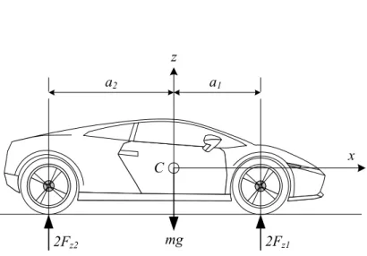
When a car is parked on level pavement, the normal force,Fz, under each of the front and rear wheels,Fz1,Fz2, are
Fz1= 1 2mg a2 l (2.1) Fz2= 1 2mg a1 l (2.2)
where, a1is the distance of the car’s mass center, C, from the front axle,
a2 is the distance ofCfrom the rear axle, and lis the wheel base.
l=a1+a2 (2.3) a1 a2 2Fz2 2Fz1 x z C mg
Proof.Consider a longitudinally symmetrical car as shown in Figure 2.1. It can be modeled as a two-axel vehicle. A symmetric two-axel vehicle is equivalent to a rigid beam having two supports. The vertical force under the front and rear wheels can be determined using planar static equilibrium equations.
X
Fz= 0 (2.4)
X
My = 0 (2.5)
Applying the equilibrium equations
2Fz1+ 2Fz2−mg= 0 (2.6)
−2Fz1a1+ 2Fz2a2= 0 (2.7)
provide the reaction forces under the front and rear tires. Fz1 = 1 2mg a2 a1+a2 =1 2mg a2 l (2.8) Fz2 = 1 2mg a1 a1+a2 =1 2mg a1 l (2.9)
Example 39 Reaction forces under wheels.
A car has 890 kg mass. Its mass center, C, is 78 cm behind the front wheel axis, and it has a 235 cmwheel base.
a1= 0.78 m (2.10)
l= 2.35 m (2.11)
m= 890 kg (2.12)
The force under each front wheel is Fz1 = 1 2mg a2 l = 1 2890×9.81× 2.35−0.78 2.35 = 2916.5 N (2.13)
and the force under each rear wheel is Fz2 = 1 2mg a1 l = 1 2890×9.81× 0.78 2.35 = 1449 N. (2.14)
Example 40 Mass center position.
Equations (2.1) and (2.2) can be rearranged to calculate the position of mass center. a1= 2l mgFz2 (2.15) a2= 2l mgFz1 (2.16)
Reaction forces under the front and rear wheels of a horizontally parked car, with a wheel basel= 2.34 m, are:
Fz1 = 2000 N (2.17)
Fz2 = 1800 N (2.18)
Therefore, the longitudinal position of the car’s mass center is at a1= 2l mgFz2 = 2 2.34 2 (2000 + 1800)×1800 = 1.1084 m (2.19) a2= 2l mgFz1 = 2 2.34 2 (2000 + 1800)×2000 = 1.2316 m. (2.20)
Example 41 Longitudinal mass center determination.
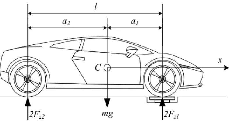
The position of mass center C can be determined experimentally. To determine the longitudinal position ofC, we should measure the total weight of the car as well as the force under the front or the rear wheels. Figure 2.2 illustrates a situation in which we measure the force under the front wheels. Assuming the force under the front wheels is 2Fz1, the position of the
mass center is calculated by static equilibrium conditions X
Fz= 0 (2.21)
X
My= 0. (2.22)
Applying the equilibrium equations
2Fz1+ 2Fz2−mg= 0 (2.23)
l 2Fz2 2Fz1 x C mg a1 a2
FIGURE 2.2. Measuring the force under the front wheels.
provide the longitudinal position ofCand the reaction forces under the rear wheels. a1= 2l mgFz2 = 2l mg (mg−2Fz1) (2.25) Fz2 = 1 2(mg−2Fz1) (2.26)
Example 42 Lateral mass center determination.
Most cars are approximately symmetrical about the longitudinal center plane passing the middle of the wheels, and therefore, the lateral position of the mass centerCis close to the center plane. However, the lateral position of C may be calculated by weighing one side of the car.
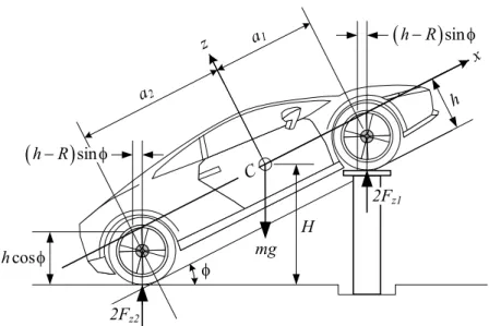
Example 43 Height mass center determination.
To determine the height of mass center C, we should measure the force under the front or rear wheels while the car is on an inclined surface. Ex-perimentally, we use a device such as is shown in Figure 2.3. The car is parked on a level surface such that the front wheels are on a scale jack. The front wheels will be locked and anchored to the jack, while the rear wheels will be left free to turn. The jack lifts the front wheels and the required vertical force applied by the jacks is measured by a load cell.
Assume that we have the longitudinal position ofC and the jack is lifted such that the car makes an angle φ with the horizontal plane. The slope angle φ is measurable using level meters. Assuming the force under the front wheels is 2Fz1, the height of the mass center can be calculated by
x z mg a2 a1 2Fz2 h φ H 2Fz1 C cos h φ
(
h R−)
sinφ(
h R−)
sinφFIGURE 2.3. Measuring the force under the wheels tofind the height of the mass center.
static equilibrium conditions X
FZ= 0 (2.27)
X
My= 0. (2.28)
Applying the equilibrium equations
2Fz1+ 2Fz2−mg = 0 (2.29)
−2Fz1(a1cosφ−(h−R) sinφ)
+2Fz2(a2cosφ+ (h−R) sinφ) = 0 (2.30)
provides the vertical position of C and the reaction forces under the rear wheels.
Fz2 = 1
2mg−Fz1 (2.31)
h= Fz1(Rsinφ+a1cosφ) +Fz2(Rsinφ−a2cosφ)
mgsinφ =R+a1Fz1−a2Fz2 mg cotφ =R+ µ 2Fz1 mg l−a2 ¶ cotφ (2.32)
A car with the following specifications m = 2000 kg 2Fz1 = 18000 N φ = 30 deg≈0.5236 rad (2.33) a1 = 110 cm l = 230 cm R = 30 cm has a C at height h. h= 34 cm (2.34)
There are three assumptions in this calculation:1−the tires are assumed to be rigid disks with radiusR,2−fluid shift, such as fuel, coolant, and oil, are ignored, and3−suspension deflections are assumed to be zero.
Suspension deflection generates the maximum effect on height determi-nation error. To eliminate the suspension deflection, we should lock the suspension, usually by replacing the shock absorbers with rigid rods to keep the vehicle at its ride height.
Example 44 Different front and rear tires.
Depending on the application, it is sometimes necessary to use different type of tires and wheels for front and rear axles. When the longitudinal position ofC for a symmetric vehicle is determined, we canfind the height of C by measuring the load on only one axle. As an example, consider the motorcycle in Figure 2.4. It has different front and rear tires.
Assume the load under the rear wheel of the motorcycle Fz is known. The heighthofC can be found by taking a moment of the forces about the tireprint of the front tire.
h=Fz2(a1+a2) mg −a1cos µ sin−1 H a1+a2 ¶ +Rf+Rr 2 (2.35)
Example 45 Statically indeterminate.
A vehicle with more than three wheels is statically indeterminate. To determine the vertical force under each tire, we need to know the mechanical properties and conditions of the tires, such as the value of deflection at the center of the tire, and its vertical stiffness.
2.2
Parked Car on an Inclined Road
When a car is parked on an inclined pavement as shown in Figure 2.5, the normal force,Fz, under each of the front and rear wheels,Fz1,Fz2, is:
C mg Fz2 Rf φ h Fz1 Rr H a2 a1
FIGURE 2.4. A motorcycle with different front and rear tires.
Fz1 = 1 2mg a2 l cosφ+ 1 2mg h l sinφ (2.36) Fz2 = 1 2mg a1 l cosφ− 1 2mg h l sinφ (2.37) l=a1+a2
where, φis the angle of the road with the horizon. The horizon is perpen-dicular to the gravitational accelerationg.
Proof.Consider the car shown in Figure 2.5. Let us assume the parking brake forces are applied on only the rear tires. It means the front tires are free to spin. Applying the planar static equilibrium equations
X Fx= 0 (2.38) X Fz= 0 (2.39) X My = 0 (2.40) shows that 2Fx2−mgsinφ= 0 (2.41) 2Fz1+ 2Fz2−mgcosφ= 0 (2.42) −2Fz1a1+ 2Fz2a2−2Fx2h= 0. (2.43)
2Fx2 2Fz1 x z C mg a2 a1 2Fz2 h a φ
FIGURE 2.5. A parked car on inclined pavement.
These equations provide the brake force and reaction forces under the front and rear tires.
Fz1 = 1 2mg a2 l cosφ− 1 2mg h l sinφ (2.44) Fz2 = 1 2mg a1 l cosφ+ 1 2mg h l sinφ (2.45) Fx2 = 1 2mgsinφ (2.46)
Example 46 Increasing the inclination angle.
Whenφ= 0, Equations (2.36) and (2.37) reduce to (2.1) and (2.2). By increasing the inclination angle, the normal force under the front tires of a parked car decreases and the normal force and braking force under the rear tires increase. The limit for increasing φ is where the weight vector mggoes through the contact point of the rear tire with the ground. Such an angle is called atilting angle.
Example 47 Maximum inclination angle.
The required braking force Fx2 increases by the inclination angle.
Be-cause Fx2 is equal to the friction force between the tire and pavement, its
maximum depends on the tire and pavement conditions. There is a specific angleφM at which the braking forceFx2 will saturate and cannot increase
any more. At this maximum angle, the braking force is proportional to the normal force Fz2
where, the coefficientμx2 is thex-direction friction coefficient for the rear wheel. Atφ=φM, the equilibrium equations will reduce to
2μx2Fz2−mgsinφM = 0 (2.48)
2Fz1+ 2Fz2−mgcosφM = 0 (2.49)
2Fz1a1−2Fz2a2+ 2μx2Fz2h= 0. (2.50)
These equations provide Fz1 = 1 2mg a2 l cosφM− 1 2mg h l sinφM (2.51) Fz2 = 1 2mg a1 l cosφM+ 1 2mg h l sinφM (2.52) tanφM = a1μx2 l−μx2h (2.53)
showing that there is a relation between the friction coefficient μx2, max-imum inclination φM, and the geometrical position of the mass center C. The angle φM increases by decreasingh.
For a car having the specifications μx2 = 1
a1 = 110 cm (2.54)
l = 230 cm
h = 35 cm
the tilting angle is
φM ≈0.514 rad≈29.43 deg. (2.55)
Example 48 Front wheel braking.
When the front wheels are the only braking wheelsFx2 = 0andFx16= 0.
In this case, the equilibrium equations will be
2Fx1−mgsinφ= 0 (2.56) 2Fz1+ 2Fz2−mgcosφ= 0 (2.57)
−2Fz1a1+ 2Fz2a2−2Fx1h= 0. (2.58)
These equations provide the brake force and reaction forces under the front and rear tires.
Fz1 = 1 2mg a2 l cosφ− 1 2mg h l sinφ (2.59) Fz2 = 1 2mg a1 l cosφ+ 1 2mg h l sinφ (2.60) Fx1 = 1 2mgsinφ (2.61)
At the ultimate angleφ=φM Fx1 =μx1Fz1 (2.62) and 2μx1Fz1−mgsinφM = 0 (2.63) 2Fz1+ 2Fz2−mgcosφM = 0 (2.64) 2Fz1a1−2Fz2a2+ 2μx1Fz1h= 0. (2.65)
These equations provide Fz1 = 1 2mg a2 l cosφM− 1 2mg h l sinφM (2.66) Fz2 = 1 2mg a1 l cosφM+ 1 2mg h l sinφM (2.67) tanφM = a2μx1 l−μx1h. (2.68)
Let’s name the ultimate angle for the front wheel brake in Equation (2.53) asφMf, and the ultimate angle for the rear wheel brake in Equation (2.68) asφMr. Comparing φMf andφMr shows that
φMf φMr = a1μx2 ¡ l−μx1h¢ a2μx1 ¡ l−μx2h¢. (2.69)
We may assume the front and rear tires are the same and so,
μx1=μx2 (2.70) therefore, φMf φMr = a1 a2 . (2.71)
Hence, if a1 < a2 then φMf < φMr and therefore, a rear brake is more
effective than a front brake on uphill parking as long asφMr is less than the tilting angle,φMr <tan−1a2
h. At the tilting angle, the weight vector passes through the contact point of the rear wheel with the ground.
Similarly we may conclude that when parked on a downhill road, the front brake is more effective than the rear brake.
Example 49 Four-wheel braking.
Consider a four-wheel brake car, parked uphill as shown in Figure 2.6. In these conditions, there will be two brake forces Fx1 on the front wheels
2Fx1 2Fx2 2Fz1 x z C mg a2 a1 2Fz2 h a φ
FIGURE 2.6. A four wheel brake car, parked uphill. The equilibrium equations for this car are
2Fx1+ 2Fx2−mgsinφ= 0 (2.72) 2Fz1+ 2Fz2−mgcosφ= 0 (2.73)
−2Fz1a1+ 2Fz2a2−(2Fx1+ 2Fx2)h= 0. (2.74)
These equations provide the brake force and reaction forces under the front and rear tires.
Fz1= 1 2mg a2 l cosφ− 1 2mg h l sinφ (2.75) Fz2= 1 2mg a1 l cosφ+ 1 2mg h l sinφ (2.76) Fx1+Fx2= 1 2mgsinφ (2.77)
At the ultimate angleφ=φM, all wheels will begin to slide simultaneously and therefore,
Fx1 = μx1Fz1 (2.78)
Fx2 = μx2Fz2. (2.79)
The equilibrium equations show that
2μx1Fz1+ 2μx2Fz2−mgsinφM = 0 (2.80) 2Fz1+ 2Fz2−mgcosφM = 0 (2.81) −2Fz1a1+ 2Fz2a2− ¡ 2μx1Fz1+ 2μx2Fz2 ¢ h= 0. (2.82)
a1 a2 2Fz2 2Fz1 x z C mg 2Fx1 h a 2Fx2
FIGURE 2.7. An accelerating car on a level pavement. Assuming μx1 =μx2=μx (2.83) will provide Fz1 = 1 2mg a2 l cosφM− 1 2mg h l sinφM (2.84) Fz2 = 1 2mg a1 l cosφM+ 1 2mg h l sinφM (2.85) tanφM =μx. (2.86)
2.3
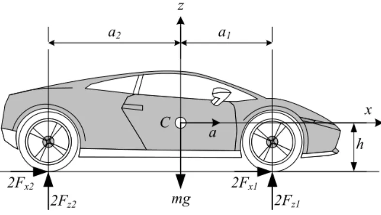
Accelerating Car on a Level Road
When a car is speeding with acceleration a on a level road as shown in Figure 2.7, the vertical forces under the front and rear wheels are
Fz1 = 1 2mg a2 l − 1 2mg h l a g (2.87) Fz2 = 1 2mg a1 l + 1 2mg h l a g. (2.88) Thefirst terms, 12mga2 l and 1 2mg a1
l , are calledstatic parts, and the second terms±12mghlag are called dynamic parts of the normal forces.
Proof.The vehicle is considered as a rigid body that moves along a hor-izontal road. The force at the tireprint of each tire may be decomposed to a normal and a longitudinal force. The equations of motion for the ac-celerating car come from Newton’s equation in x-direction and two static
equilibrium equations. X Fx=ma (2.89) X Fz= 0 (2.90) X My = 0. (2.91)
Expanding the equations of motion produces three equations for four unknownsFx1,Fx2,Fz1,Fz2.
2Fx1+ 2Fx2=ma (2.92) 2Fz1+ 2Fz2−mg= 0 (2.93)
−2Fz1a1+ 2Fz2a2−2 (Fx1+Fx2)h= 0 (2.94)
However, it is possible to eliminate(Fx1+Fx2)between thefirst and third
equations, and solve for the normal forcesFz1,Fz2.
Fz1 = (Fz1)st+ (Fz1)dyn = 1 2mg a2 l − 1 2mg h l a g (2.95) Fz2 = (Fz2)st+ (Fz2)dyn = 1 2mg a1 l + 1 2mg h l a g (2.96)
The static parts
(Fz1)st = 1 2mg a2 l (2.97) (Fz2)st = 1 2mg a1 l (2.98)
are weight distribution for a stationary car and depend on the horizontal position of the mass center. However, the dynamic parts
(Fz1)dyn = − 1 2mg h l a g (2.99) (Fz2)dyn = 1 2mg h l a g (2.100)
indicate the weight distribution according to horizontal acceleration, and depend on the vertical position of the mass center.
When acceleratinga >0, the normal forces under the front tires are less than the static load, and under the rear tires are more than the static load.
Example 50 Front-wheel-drive accelerating on a level road.
When the car is front-wheel-drive, Fx2 = 0. Equations (2.92) to (2.88)
will provide the same vertical tireprint forces as (2.87) and (2.88). However, the required horizontal force to achieve the same acceleration, a, must be provided by solely the front wheels.
Example 51 Rear-wheel drive accelerating on a level road.
If a car is rear-wheel drive then,Fx1 = 0and the required force to achieve
the acceleration, a, must be provided only by the rear wheels. The vertical force under the wheels will still be the same as (2.87) and (2.88).
Example 52 Maximum acceleration on a level road.
The maximum acceleration of a car is proportional to the friction under its tires. We assume the friction coefficients at the front and rear tires are equal and all tires reach their maximum tractions at the same time.
Fx1 = ±μxFz1 (2.101)
Fx2 = ±μxFz2 (2.102)
Newton’s equation (2.92) can now be written as
ma=±2μx(Fz1+Fz2). (2.103)
SubstitutingFz1 and Fz2 from (2.93) and (2.94) results in
a=±μxg. (2.104)
Therefore, the maximum acceleration and deceleration depend directly on the friction coefficient.
Example 53 Maximum acceleration for a single-axle drive car.
The maximum acceleration arwd for a rear-wheel-drive car is achieved when we substitute Fx1 = 0, Fx2 = μxFz2 in Equation (2.92) and use
Equation (2.88) μxmg µ a1 l + h l arwd g ¶ =marwd (2.105) and therefore, arwd g = a1μx l−hμx = μx 1−μxh l a1 l . (2.106)
The front wheels can leave the ground when Fz1 = 0. SubstitutingFz1 = 0
in Equation (2.88) provides the maximum acceleration at which the front wheels are still on the road.
arwd g ≤
a2
a1/l
a/g
arwd/g afwd
/g
FIGURE 2.8. Effect of mass center position on the maximum achievable acceler-ation of a front- and a rear-wheel drive car.
Therefore, the maximum attainable acceleration would be the less value of Equation (2.106) or (2.107).
Similarly, the maximum acceleration af wd for a front-wheel drive car is achieved when we substitute Fx2 = 0,Fx1 =μxFz1 in Equation (2.92) and
use Equation (2.87). af wd g = a2μx l+hμx = μx 1 +μxh l ³ 1−a1 l ´ (2.108) To see the effect of changing the position of mass center on the maximum achievable acceleration, we plot Figure 2.8 for a sample car with
μx = 1
h = 0.56 m (2.109)
l = 2.6 m.
Passenger cars are usually in the range0.4<(a1/g)<0.6, with(a1/g)→
0.4for front-wheel-drive cars, and(a1/g)→0.6 for rear-wheel-drive cars.
In this range,(arwd/g)>(af wd/g)and therefore rear-wheel-drive cars can reach higher forward acceleration than front-wheel-drive cars. It is an im-portant applied fact, especially for race cars.
The maximum acceleration may also be limited by the tilting condition aM
g ≤ a2
Example 54 Minimum time for0−100 km/h on a level road. Consider a car with the following characteristics:
length = 4245 mm width = 1795 mm height = 1285 mm wheel base = 2272 mm f ront track = 1411 mm (2.111) rear track = 1504 mm net weight = 1500 kg h = 220 mm μx = 1 a1 = a2
Assume the car is rear-wheel-drive and its engine can provide the maximum traction supported by friction. Equation (2.88) determines the load on the rear wheels and therefore, the forward equation of motion is
2Fx2 = 2μxFz2 = μxmga1 l +μxmg h l 1 ga = m a. (2.112)
Rearrangement provides the following differential equation to calculate ve-locity and displacement:
a = x¨= μxga1 l 1−μxgh l 1 g = gμx a1 l−hμx (2.113) Taking an integral Z 27.78 0 dv= Z t 0 a dt (2.114)
between v = 0 and v = 100 km/h ≈ 27.78 m/s shows that the minimum time for0−100 km/h on a level road is
t= 27.78
gμx a1 l−hμx
If the same car was front-wheel-drive, then the traction force would be 2Fx1 = 2μxFz1 = μxmga2 l −μxmg h l 1 ga = m a. (2.116)
and the equation of motion would reduce to
a = x¨= μxga2 l 1 +μxgh l 1 g = gμx a2 l+hμx. (2.117)
The minimum time for0−100 km/h on a level road for this front-wheel-drive car is
t= 27.78
gμx a2 l+hμx
≈6.21 s. (2.118)
Now consider the same car to be four-wheel-drive. Then, the traction force is
2Fx1+ 2Fx2 = 2μx (Fz1+Fz2)
= g
lm(a1+a2)
= m a. (2.119)
and the minimum time for0−100 km/hon a level road for this four-wheel-drive car can theoretically be reduced to
t=27.78
g ≈2.83 s. (2.120)
2.4
Accelerating Car on an Inclined Road
When a car is accelerating on an inclined pavement with angleφas shown in Figure 2.9, the normal force under each of the front and rear wheels, Fz1,Fz2, would be: Fz1= 1 2mg µ a2 l cosφ− h l sinφ ¶ −12mah l (2.121) Fz2= 1 2mg µ a1 l cosφ+ h l sinφ ¶ +1 2ma h l (2.122) l=a1+a2
2Fx2 2Fz1 x z C mg a2 a1 2Fz2 h a 2Fx1 φ
FIGURE 2.9. An accelerating car on inclined pavement.
The dynamic parts, ±12mghlag, depend on acceleration a and height hof mass centerC and remain unchanged, while the static parts are influenced by the slope angleφand height hof mass center.
Proof. The Newton’s equation in x-direction and two static equilibrium equations, must be examined to find the equation of motion and ground reaction forces. X Fx=ma (2.123) X Fz= 0 (2.124) X My = 0. (2.125)
Expanding these equations produces three equations for four unknowns Fx1,Fx2,Fz1,Fz2.
2Fx1+ 2Fx2−mgsinφ=ma (2.126) 2Fz1+ 2Fz2−mgcosφ= 0 (2.127) 2Fz1a1−2Fz2a2+ 2 (Fx1+Fx2)h= 0 (2.128)
It is possible to eliminate(Fx1+Fx2)between thefirst and third equations,
and solve for the normal forcesFz1,Fz2.
Fz1 = (Fz1)st+ (Fz1)dyn = 1 2mg µ a2 l cosφ− h l sinφ ¶ −12mah l (2.129)
Fz2 = (Fz2)st+ (Fz2)dyn = 1 2mg µ a1 l cosφ+ h l sinφ ¶ +1 2ma h l (2.130)
Example 55 Front-wheel-drive car, accelerating on inclined road.
For a front-wheel-drive car, we may substitute Fx1 = 0 in Equations
(2.126) and (2.128) to have the governing equations. However, it does not affect the ground reaction forces under the tires (2.129 and 2.130) as long as the car is driven under its limit conditions.
Example 56 Rear-wheel-drive car, accelerating on inclined road.
SubstitutingFx2 = 0in Equations (2.126) and (2.128) and solving for the
normal reaction forces under each tire provides the same results as (2.129) and (2.130). Hence, the normal forces applied on the tires do not sense if the car is front-, rear-, or all-wheel drive. As long as we drive in a straight path at low acceleration, the drive wheels can be the front or the rear ones. However, the advantages and disadvantages of front-, rear-, or all-wheel drive cars appear in maneuvering, slippery roads, or when the maximum acceleration is required.
Example 57 Maximum acceleration on an inclined road.
The maximum acceleration depends on the friction under the tires. Let’s assume the friction coefficients at the front and rear tires are equal. Then, the front and rear traction forces are
Fx1 ≤ μxFz1 (2.131)
Fx2 ≤ μxFz2. (2.132)
If we assume the front and rear wheels reach their traction limits at the same time, then
Fx1 = ±μxFz1 (2.133)
Fx2 = ±μxFz2 (2.134)
and we may rewrite Newton’s equation (2.123) as
maM =±2μx(Fz1+Fz2)−mgsinφ (2.135)
where,aM is the maximum achievable acceleration.
Now substituting Fz1 andFz2 from (2.129) and (2.130) results in
aM
g =±μxcosφ−sinφ. (2.136) Accelerating on an uphill road (a >0, φ >0) and braking on a downhill road (a <0, φ <0) are the extreme cases in which the car can stall. In these cases, the car can move as long as
Example 58 Limits of acceleration and inclination angle.
Assuming Fz1 > 0 and Fz2 > 0, we can write Equations (2.121) and
(2.122) as a g ≤ a2 h cosφ−sinφ (2.138) a g ≥ − a1 h cosφ−sinφ. (2.139)
Hence, the maximum achievable acceleration (a >0)is limited bya2,h,φ;
while the maximum deceleration (a <0) is limited by a1, h, φ. These two
equations can be combined to result in −a1 h cosφ≤ a g + sinφ≤ a2 h cosφ. (2.140)
If a→0, then the limits of the inclination angle would be −ah1 ≤tanφ≤a2
h. (2.141)
This is the maximum and minimum road inclination angles that the car can stay on without tilting and falling.
Example 59 Maximum deceleration for a single-axle-brake car.
We can find the maximum braking deceleration af wb of a front-wheel-brake car on a horizontal road by substituting φ = 0, Fx2 = 0, Fx1 =
−μxFz1 in Equation (2.126) and using Equation (2.121)
−μxmg µ a2 l − h l arwb g ¶ =maf wb (2.142) therefore, af wb g =− μx 1−μxh l ³ 1−a1 l ´ . (2.143)
Similarly, the maximum braking deceleration arwb of a front-wheel-brake car can be achieved when we substituteFx2 = 0,Fx1=μxFz1.
arwb g =− μx 1 +μxh l a1 l (2.144)
The effect of changing the position of the mass center on the maximum achievable braking deceleration is shown in Figure 2.10 for a sample car with
μx = 1
h = 0.56 m (2.145)
a1/l
a/g
afwd/g
arwd/g
FIGURE 2.10. Effect of mass center position on the maximum achievable deccel-eration of a front-wheel and a rear-wheel-drive car.
Passenger cars are usually in the range0.4<(a1/l)<0.6. In this range,
(af wb/g)<(arwb/g)and therefore, front-wheel-brake cars can reach better forward deceleration than rear-wheel-brake cars. Hence, front brakes are much more important than the rear brakes.
Example 60 FA car with a trailer.
Figure 2.11 depicts a car moving on an inclined road and pulling a trailer. To analyze the car-trailer motion, we need to separate the car and trailer to see the forces at the hinge, as shown in Figure 2.12. We assume the mass center of the trailer Ct is at distance b3 in front of the only axle of
the trailer. IfCtis behind the trailer axle, thenb3 should be negative in the
following equations.
For an ideal hinge between a car and a trailer moving in a straight path, there must be a horizontal forceFxt and a vertical forceFzt.
Writing the Newton’s equation inx-direction and two static equilibrium equations for both the trailer and the vehicle
X Fx=mta (2.146) X Fz= 0 (2.147) X My= 0 (2.148)
wefind the following set of equations:
Fxt−mtgsinφ=mta (2.149) 2Fz3−Fzt−mtgcosφ= 0 (2.150) 2Fz3b3−Fztb2−Fxt(h2−h1) = 0 (2.151)
2Fx2 2Fz1 x z C mg a2 a1 2Fz2 h a 2Fx1 φ Ct mtg b2 b1 b3 2Fz3
FIGURE 2.11. A car moving on an inclined road and pulling a trailer.
2Fx1+ 2Fx2−Fxt −mgsinφ=ma (2.152) 2Fz1+ 2Fz2−Fzt−mgcosφ= 0 (2.153) 2Fz1a1−2Fz2a2+ 2 (Fx1+Fx2)h
−Fxt(h−h1) +Fzt(b1+a2) = 0 (2.154)
If the value of traction forcesFx1andFx2 are given, then these are six
equa-tions for six unknowns: a,Fxt,Fzt,Fz1,Fz2,Fz3. Solving these equations
provide the following solutions:
a = 2 m+mt (Fx1+Fx2)−gsinφ (2.155) Fxt = 2mt m+mt (Fx1+Fx2) (2.156) Fzt = h1−h2 b2−b3 2mt m+mt (Fx1+Fx2) + b3 b2−b3 mtgcosφ (2.157) Fz1 = b3 2l µ 2a2−b1 b2−b3 mt+ a2 b3 m ¶ gcosφ + ∙ 2a2−b1 b2−b3 (h1−h2)mt−h1mt−hm ¸ Fx1+Fx2 l(m+mt) (2.158)
Fzt 2F x2 2Fz1 x z C mg 2Fz2 h a 2Fx1 φ Ct mt g Fxt Fzt Fxt φ 2Fz3 h1 h1 h 2 a1 a2 b1 b2 b3
FIGURE 2.12. Free-body-diagram of a car and the trailer when moving on an uphill road. Fz2 = b3 2l µ a1−a2+b1 b2−b3 mt+ a1 b3 m ¶ gcosφ + ∙ a1−a2+b1 b2−b3 (h1−h2)mt+h1mt+hm ¸ Fx1+Fx2 l(m+mt) (2.159) Fz3 = 1 2 b2 b2−b3 mtgcosφ+ h1−h2 b2−b3 mt m+mt (Fx1+Fx2) (2.160) l = a1+a2. (2.161)
However, if the value of accelerationais known, then unknowns are:Fx1+
Fx2,Fxt,Fzt,Fz1,Fz2,Fz3. Fx1+Fx2 = 1 2(m+mt) (a+gsinφ) (2.162) Fxt = mt(a+gsinφ) (2.163) Fzt = h1−h2 b2−b3 mt(a+gsinφ) + b3 b2−b3 mtgcosφ (2.164)
Fz1 = b3 2l µ 2a2−b1 b2−b3 mt+ a2 b3 m ¶ gcosφ (2.165) +1 2l ∙ 2a2−b1 b2−b3 (h1−h2)mt−h1mt−hm ¸ (a+gsinφ) Fz2 = b3 2l µ a1−a2+b1 b2−b3 mt+ a1 b3 m ¶ gcosφ (2.166) +1 2l ∙ a1−a2+b1 b2−b3 (h1−h2)mt+h1mt+hm ¸ (a+gsinφ) Fz3 = 1 2 mt b2−b3 (b2gcosφ+ (h1−h2) (a+gsinφ)) (2.167) l = a1+a2.
Example 61 FMaximum inclination angle for a car with a trailer. For a car and trailer as shown in Figure 2.11, the maximum inclina-tion angle φM is the angle at which the car cannot accelerate the vehicle. Substitutinga= 0 andφ=φM in Equation (2.155) shows that
sinφM = 2
(m+mt)g
(Fx1+Fx2). (2.168)
The value of maximum inclination angle φM increases by decreasing the total weight of the vehicle and trailer(m+mt)gor increasing the traction forceFx1+Fx2.
The traction force is limited by the maximum torque on the drive wheel and the friction under the drive tire. Let’s assume the vehicle is four-wheel-drive and friction coefficients at the front and rear tires are equal. Then, the front and rear traction forces are
Fx1 ≤ μxFz1 (2.169)
Fx2 ≤ μxFz2. (2.170)
If we assume the front and rear wheels reach their traction limits at the same time, then
Fx1 = μxFz1 (2.171)
Fx2 = μxFz2 (2.172)
and we may rewrite the Equation (2.168) as
sinφM =
2μx
(m+mt)g
(Fz1+Fz2). (2.173)
Now substituting Fz1 andFz2 from (2.158) and (2.159) results in (mb3−mb2−mtb3)μxcosφM+ (b2−b3) (m+mt) sinφM
= 2μxmt(h1−h2) m+mt
If we arrange Equation (2.174) as AcosφM +BsinφM =C (2.175) then φM = atan2( C √ A2+B2,± r 1− C 2 A2+B2)−atan2(A, B) (2.176) and φM = atan2(√ C A2+B2,± p A2+B2−C2)−atan2(A, B) (2.177) where A = (mb3−mb2−mtb3)μx (2.178) B = (b2−b3) (m+mt) (2.179) C = 2μxmt(h1−h2) m+mt (Fx1+Fx2). (2.180)
For a rear-wheel-drive car pulling a trailer with the following character-istics: l = 2272 mm w = 1457 mm h = 230 mm a1 = a2 h1 = 310 mm b1 = 680 mm b2 = 610 mm b3 = 120 mm (2.181) h2 = 560 mm m = 1500 kg mt = 150 kg μx = 1 φ = 10 deg a = 1 m/s2 wefind Fz1 = 3441.78 N Fz2 = 3877.93 N Fz3 = 798.57 N Fzt = 147.99 N (2.182) Fxt = 405.52 N Fx2 = 2230.37 N.
To check if the required traction force Fx2 is applicable, we should compare
it to the maximum available friction forceμFz2 and it must be
Fx2≤μFz2. (2.183)
Example 62 FSolution of equationacosθ+bsinθ=c. The first type of trigonometric equation is
acosθ+bsinθ=c. (2.184) It can be solved by introducing two new variables randη such that
a = rsinη (2.185)
b = rcosη (2.186)
and therefore,
r = pa2+b2 (2.187)
η = atan2(a, b). (2.188)
Substituting the new variables show that
sin(η+θ) = c r (2.189) cos(η+θ) = ± r 1−c 2 r2. (2.190)
Hence, the solutions of the problem are θ= atan2(c r,± r 1−c 2 r2)−atan2(a, b) (2.191) and θ= atan2(c r,± p r2−c2)−atan2(a, b). (2.192)
Therefore, the equation acosθ+bsinθ = c has two solutions if r2 =
a2+b2> c2, one solution ifr2=c2, and no solution if r2< c2.
Example 63 FThe function tan−21xy = atan2(y, x).
There are many situations in kinematics calculation in which we need tofind an angle based on thesin andcos functions of an angle. However,
tan−1 cannot show the effect of the individual sign for the numerator and denominator. It always represents an angle in the first or fourth quadrant. To overcome this problem and determine the angle in the correct quadrant, theatan2function is introduced as below.
atan2(y, x) = ⎧ ⎪ ⎪ ⎪ ⎪ ⎪ ⎨ ⎪ ⎪ ⎪ ⎪ ⎪ ⎩ tan−1y x if y >0 tan−1y x+πsigny if y <0 π 2signx if y= 0 (2.193)
In this text, whether it has been mentioned or not, wherever tan−1yx is used, it must be calculated based onatan2(y, x).
Example 64 Zero vertical force at the hinge.
We can make the vertical force at the hinge equal to zero by examining Equation (2.157) for the hinge vertical forceFzt.
Fzt = h1−h2 b2−b3 2mt m+mt (Fx1+Fx2) + b3 b2−b3 mtgcosφ (2.194) To make Fzt = 0, it is enough to adjust the position of trailer mass center
Ctexactly on top of the trailer axle and at the same height as the hinge. In these conditions we have
h1 = h2 (2.195)
b3 = 0 (2.196)
that makes
Fzt = 0. (2.197)
However, to increase safety, the load should be distributed evenly through-out the trailer. Heavy items should be loaded as low as possible, mainly over the axle. Bulkier and lighter items should be distributed to give a little pos-itiveb3. Such a trailer is called nose weight at the towing coupling.
2.5
Parked Car on a Banked Road
Figure 2.13 depicts the effect of a bank angleφon the load distribution of a vehicle. A bank causes the load on the lower tires to increase, and the load on the upper tires to decrease. The tire reaction forces are:
Fz1 = 1 2 mg w (b2cosφ−hsinφ) (2.198) Fz2 = 1 2 mg w (b1cosφ+hsinφ) (2.199) w=b1+b2 (2.200)
Proof.Starting with equilibrium equations X Fy = 0 (2.201) X Fz= 0 (2.202) X Mx= 0. (2.203)
2Fy2 2Fz1 y z C mg b2 b1 2Fz2 h 2Fy1 φ
FIGURE 2.13. Normal force under the uphill and downhill tires of a vehicle, parked on banked road.
we can write
2Fy1+ 2Fy2−mgsinφ= 0 (2.204) 2Fz1+ 2Fz2−mgcosφ= 0 (2.205) 2Fz1b1−2Fz2b2+ 2 (Fy1+Fy2)h= 0. (2.206)
We assumed the force under the lower tires, front and rear, are equal, and also the forces under the upper tires, front and rear are equal. To calculate the reaction forces under each tire, we may assume the overall lateral force Fy1+Fy2as an unknown. The solution of these equations provide the lateral
and reaction forces under the upper and lower tires. Fz1 = 1 2mg b2 wcosφ− 1 2mg h wsinφ (2.207) Fz2 = 1 2mg b1 wcosφ+ 1 2mg h wsinφ (2.208) Fy1+Fy2 = 1 2mgsinφ (2.209)
At the ultimate angle φ=φM, all wheels will begin to slide simultane-ously and therefore,
Fy1 = μy1Fz1 (2.210)
The equilibrium equations show that 2μy1Fz1+ 2μy2Fz2−mgsinφ= 0 (2.212) 2Fz1+ 2Fz2−mgcosφ= 0 (2.213) 2Fz1b1−2Fz2b2+ 2 ¡ μy1Fz1+μy2Fz2 ¢ h= 0. (2.214) Assuming μy1=μy2 =μy (2.215) will provide Fz1 = 1 2mg b2 wcosφM− 1 2mg h wsinφM (2.216) Fz2 = 1 2mg b1 wcosφM+ 1 2mg h wsinφM (2.217) tanφM =μy. (2.218)
These calculations are correct as long as
tanφM ≤ b2
h (2.219)
μy ≤ b2
h. (2.220)
If the lateral frictionμy is higher thanb2/hthen the car will roll downhill.
To increase the capability of a car moving on a banked road, the car should be as wide as possible with a mass center as low as possible.
Example 65 Tire forces of a parked car in a banked road. A car having
m = 980 kg
h = 0.6 m (2.221)
w = 1.52 m
b1 = b2
is parked on a banked road withφ= 4 deg. The forces under the lower and upper tires of the car are:
Fz1 = 2265.2 N
Fz2 = 2529.9 N (2.222)
Fy1+Fy2 = 335.3 N
The ratio of the uphill force Fz1 to downhill force Fz2 depends on only
the mass center position. Fz1
Fz2
= b2cosφ−hsinφ
b1cosφ+hsinφ
1 2 z z F F φ φ[deg] h=0.6 m w=1.52 m b1=b2 Rolling down angle
[rad]
FIGURE 2.14. Illustration of the force ratioFz1/Fz2 as a function of road bank
angleφ.
Assuming a symmetric car withb1=b2=w/2simplifies the equation to
Fz1
Fz2
=wcosφ−2hsinφ
wcosφ+ 2hsinφ. (2.224) Figure 2.14 illustrates the behavior of force ratioFz1/Fz2 as a function ofφ
forh= 0.6 mandw= 1.52 m. The rolling down angleφM = tan−1(b2/h) =
51.71 degindicates the bank angle at which the force under the uphill wheels become zero and the car rolls down. The negative part of the curve indicates the required force to keep the car on the road, which is not applicable in real situations.
2.6
F
Optimal Drive and Brake Force Distribution
A certain acceleration acan be achieved by adjusting and controlling the longitudinal forcesFx1 andFx2. The optimal longitudinal forces under thefront and rear tires to achieve the maximum acceleration are Fx1 mg = − 1 2 h l µ a g ¶2 +1 2 a2 l a g = −1 2μ 2 x h l + 1 2μx a2 l (2.225)
Fx2 mg = 1 2 h l µa g ¶2 +1 2 a1 l a g = 1 2μ 2 x h l + 1 2μx a1 l . (2.226)
Proof.The longitudinal equation of motion for a car on a horizontal road is
2Fx1+ 2Fx2=ma (2.227)
and the maximum traction forces under each tire is a function of normal force and the friction coefficient.
Fx1 ≤ ±μxFz1 (2.228)
Fx2 ≤ ±μxFz2 (2.229)
However, the normal forces are a function of the car’s acceleration and geometry. Fz1 = 1 2mg a2 l − 1 2mg h l a g (2.230) Fz2 = 1 2mg a1 l + 1 2mg h l a g (2.231)
We may generalize the equations by making them dimensionless. Under the best conditions, we should adjust the traction forces to their maximum
Fx1 mg = 1 2μx µ a2 l − h l a g ¶ (2.232) Fx2 mg = 1 2μx µ a1 l + h l a g ¶ (2.233) and therefore, the longitudinal equation of motion (2.227) becomes
a
g =μx. (2.234)
Substituting this result back into Equations (2.232) and (2.233) shows that Fx1 mg = − 1 2 h l µ a g ¶2 +1 2 a2 l a g (2.235) Fx2 mg = 1 2 h l µ a g ¶2 +1 2 a1 l a g. (2.236)
Depending on the geometry of the car(h, a1, a2), and the acceleration a >
0, these two equations determine how much the front and rear driving forces must be. The same equations are applied for decelerationa <0, to
a / g Fx/ mg Fx1/ mg Fx2/ mg Fx2/ mg Fx1/ mg 1 a h − 2 a h
FIGURE 2.15. Optimal driving and braking forces for a sample car. determine the value of optimal front and rear braking forces. Figure 2.15 represents a graphical illustration of the optimal driving and braking forces for a sample car using the following data:
μx = 1 h l = 0.56 2.6 = 0.21538 (2.237) a1 l = a2 l = 1 2.
When accelerating a >0, the optimal driving force on the rear tire grows rapidly while the optimal driving force on the front tire drops after a max-imum. The value (a/g) = (a2/h) is the maximum possible acceleration
at which the front tires lose their contact with the ground. The accelera-tion at which front (or rear) tires lose their ground contact is calledtilting acceleration.
The opposite phenomenon happens when decelerating. For a < 0, the optimal front brake force increases rapidly and the rear brake force goes to zero after a minimum. The deceleration(a/g) =−(a1/h)is the maximum
possible deceleration at which the rear tires lose their ground contact. The graphical representation of the optimal driving and braking forces can be shown better by plotting Fx1/(mg) versus Fx2/(mg) using (a/g)
as a parameter. Fx1 = a2− a gh a1+ a gh Fx2 (2.238) Fx1 Fx2 = a2−μxh a1+μxh (2.239)
Fx1/ mg Fx2/ mg 1 a h 2 a h Driving Br ak in g
FIGURE 2.16. Optimal traction and braking force distribution between the front and rear wheels.
Such a plot is shown in Figure 2.16. This is a design curve describing the relationship between forces under the front and rear wheels to achieve the maximum acceleration or deceleration.
Adjusting the optimal force distribution is not an automatic procedure and needs a force distributor control system to measure and adjust the forces.
Example 66 FSlope at zero.
The initial optimal traction force distribution is the slope of the optimal curve(Fx1/(mg), Fx2/(mg))at zero. dFx1 mg dFx2 mg = lim a→0 −12hl µ a g ¶2 +1 2 a2 l a g 1 2 h l µ a g ¶2 +1 2 a1 l a g = a2 a1 (2.240) Therefore, the initial traction force distribution depends on only the position of mass centerC.
Example 67 FBrake balance and ABS.
When braking, a car is stable if the rear wheels do not lock. Thus, the rear brake forces must be less than the maximum possible braking force at all time. This means the brake force distribution should always be in the shaded area of Figure 2.17, and below the optimal curve. This restricts the
Fx1/ mg Fx2/ mg 1 a h Braking
FIGURE 2.17. Optimal braking force distribution between the front and rear wheels, along with a thre-line under estimation.
achievable deceleration, especially at low friction values, but increases the stability of the car.
Whenever it is easier for a force distributor to follow a line, the optimal brake curve is underestimated using two or three lines, and a control system adjusts the force ratio Fx1/Fx2. A sample of three-line approximation is
shown in Figure 2.17.
Distribution of the brake force between the front and rear wheels is called brake balance. Brake balance varies with deceleration. The higher the stop, the more load will transfer to the front wheels and the more braking effort they can support. Meanwhile the rear wheels are unloaded and they must have less braking force.
Example 68 FBest race car.
Racecars always work at the maximum achievable acceleration to finish their race in minimum time. They are usually designed with rear-wheel-drive and all-wheel-brake. However, if an all-wheel-rear-wheel-drive race car is reason-able to build, then a force distributor, to follow the curve shown in Figure 2.18, is what it needs to race better.
Example 69 FEffect ofC location on braking.
Load is transferred from the rear wheels to the front when the brakes are applied. The higher theC, the more load transfer. So, to improve braking, the mass center C should be as low as possible and as back as possible. This is not feasible for every vehicle, especially for forward-wheel drive street cars. However, this fact should be taken into account when a car is
Fx1/ mg Fx2/ mg 2 a h Driving 0.1 0.2 0 0.2 0.4 0.6 0.8 1.0 1.2
FIGURE 2.18. Optimal traction force distribution between the front and rear wheels. v Fy1 Fx1 Fx2 Fx2 Fx1 Fy1
FIGURE 2.19.180 degsliding rotation of a rear-wheel-locked car. being designed for better braking performance.
Example 70 FFront and rear wheel locking.
The optimal brake force distribution is according to Equation (2.239) for an idealFx1/Fx2 ratio. However, if the brake force distribution is not ideal,
then either the front or the rear wheels will lock upfirst. Locking the rear wheels makes the vehicle unstable, and it loses directional stability. When the rear wheels lock, they slide on the road and they lose their capacity to support lateral force. The resultant shear force at the tireprint of the rear wheels reduces to a dynamic friction force in the opposite direction of the sliding.
A slight lateral motion of the rear wheels, by any disturbance, develops a yaw motion because of unbalanced lateral forces on the front and rear wheels. The yaw moment turns the vehicle about the z-axis until the rear end leads the front end and the vehicle turns180 deg. Figure 2.19 illustrates a180 deg sliding rotation of a rear-wheel-locked car.
The lock-up of the front tires does not cause a directional instability, although the car would not be steerable and the driver would lose control.
2.7
F
Vehicles With More Than Two Axles
If a vehicle has more than two axles, such as the three-axle car shown in Figure 2.20, then the vehicle will be statically indeterminate and the normal forces under the tires cannot be determined by static equilibrium equations. We need to consider the suspensions’ deflection to determine their applied forces.
The n normal forces Fzi under the tires can be calculated using the
followingnalgebraic equations.
2 n X i=1 Fzi−mgcosφ= 0 (2.241) 2 n X i=1 Fzixi+h(a+mgsinφ) = 0 (2.242) Fzi ki − xi−x1 xn−x1 µ Fzn kn − Fz1 k1 ¶ −Fz1 k1 = 0 for i= 2,3,· · ·, n−1 (2.243) where Fxi and Fzi are the longitudinal and normal forces under the tires
attached to the axle number i, and xi is the distance of mass center C from the axle numberi. The distancexi is positive for axles in front ofC, and is negative for the axles in back ofC. The parameterki is the vertical stiffness of the suspension at axlei.
Proof.For a multiple-axle vehicle, the following equations X Fx=ma (2.244) X Fz= 0 (2.245) X My = 0 (2.246)
provide the same sort of equations as (2.126)-(2.128). However, if the total number of axles are n, then the individual forces can be substituted by a summation. 2 n X i=1 Fxi−mgsinφ=ma (2.247) 2 n X i=1 Fzi−mgcosφ= 0 (2.248)
2Fx1 2Fx2 x z C h a 2Fz1 mg 2Fz2
φ
2Fz3 a1 a2 a3 2Fx3FIGURE 2.20. A three-axle car moving on an inclined road.
2 n X i=1 Fzixi+ 2h n X i=1 Fxi= 0 (2.249)
The overall forward force Fx = 2Pni=1Fxi can be eliminated between
Equations (2.247) and (2.249) to make Equation (2.242). Then, there re-main two equations (2.241) and (2.242) fornunknownsFzi,i= 1,2,· · · , n.
Hence, we need n−2extra equations to be able to find the wheel loads. The extra equations come from the compatibility among the suspensions’ deflection.
We ignore the tires’ compliance, and usez to indicate the static vertical displacement of the car atC. Then, ifziis the suspension deflection at the center of axle i, andki is the vertical stiffness of the suspension at axlei, the deflections are
zi= Fzi
ki
. (2.250)
For aflat road, and a rigid vehicle, we must have zi−z1
xi−x1
= zn−z1
xn−x1
for i= 2,3,· · · , n−1 (2.251) which, after substituting with (2.250), reduces to Equation (2.243). The n−2equations (2.251) along with the two equations (2.241) and (2.242) are enough to calculate the normal load under each tire. The resultant set of equations is linear and may be arranged in a matrix form
where [X] =£ Fz1 Fz2 Fz3 · · · Fzn ¤T (2.253) [A] = ⎡ ⎢ ⎢ ⎢ ⎢ ⎢ ⎢ ⎢ ⎢ ⎢ ⎢ ⎢ ⎢ ⎢ ⎣ 2 2 · · · · · · · · · · · · 2 2x1 2x2 · · · 2xn xn−x2 k1l 1 k2 · · · · x2−x1 knl · · · · xn−xi k1l · · · · 1 ki · · · · xi−x1 knl · · · · xn−xn−1 k1l · · · · 1 kn−1 xn−1−x1 knl ⎤ ⎥ ⎥ ⎥ ⎥ ⎥ ⎥ ⎥ ⎥ ⎥ ⎥ ⎥ ⎥ ⎥ ⎦ (2.254) l = x1−xn (2.255) [B] =£ mgcosφ −h(a+mgsinφ) 0 · · · 0 ¤T. (2.256)
Example 71 FWheel reactions for a three-axle car.
Figure 2.20 illustrates a three-axle car moving on an inclined road. We start counting the axles of a multiple-axle vehicle from the front axle as axle-1, and move sequentially to the back as shown in the figure.
The set of equations for the three-axle car, as seen in Figure 2.20, is
2Fx1+ 2Fx2+ 2Fx3−mgsinφ = ma (2.257) 2Fz1+ 2Fz2+ 2Fz3−mgcosφ = 0 (2.258) 2Fz1x1+ 2Fz2x2+ 2Fz3x3+ 2h(Fx1+Fx2+Fx3) = 0 (2.259) 1 x2−x1 µ Fz2 k2 − Fz1 k1 ¶ −x 1 3−x1 µ Fz3 k3 − Fz1 k1 ¶ = 0 (2.260) which can be simplified to
2Fz1+ 2Fz2+ 2Fz3−mgcosφ = 0 (2.261) 2Fz1x1+ 2Fz2x2+ 2Fz3x3+hm(a+gsinφ) = 0 (2.262) (x2k2k3−x3k2k3)Fz1+ (x1k1k2−x2k1k2)Fz3
−(x1k1k3−x3k1k3)Fz2 = 0. (2.263)
The set of equations for wheel loads is linear and may be rearranged in a matrix form
where [A] = ⎡ ⎣ 22x1 22x2 22x3 k2k3(x2−x3) k1k3(x3−x1) k1k2(x1−x2) ⎤ ⎦ (2.265) [X] = ⎡ ⎣ FFzz12 Fz3 ⎤ ⎦ (2.266) [B] = ⎡ ⎣ −hmmg(acos+gφsinφ) 0 ⎤ ⎦. (2.267)
The unknown vector may be found using matrix inversion
[X] = [A]−1[B]. (2.268) The solution of the equations are
1 k1m Fz1 = Z1 Z0 (2.269) 1 k2m Fz2 = Z2 Z0 (2.270) 1 k2m Fz3 = Z3 Z0 (2.271) where, Z0=−4k1k2(x1−x2)2−4k2k3(x2−x3)2−4k1k3(x3−x1)2 (2.272) Z1 = g(x2k2−x1k3−x1k2+x3k3)hsinφ +a(x2k2−x1k3−x1k2+x3k3)h +g¡k2x22−x1k2x2+k3x23−x1k3x3¢cosφ (2.273) Z2 = g(x1k1−x2k1−x2k3+x3k3)hsinφ +a(x1k1−x2k1−x2k3+x3k3)h +g¡k1x21−x2k1x1+k3x23−x2k3x3¢cosφ (2.274) Z3 = g(x1k1+x2k2−x3k1−x3k2)hsinφ +a(x1k1+x2k2−x3k1−x3k2)h +g¡k1x21−x3k1x1+k2x22−x3k2x2¢cosφ (2.275) x1 = a1 (2.276) x2 = −a2 (2.277) x3 = −a3. (2.278)
RH 2Fz1 x z C mg a2 a1 2Fz2 a 2Fx1 θ φ v 2Fx2
FIGURE 2.21. A cresting vehicle at a point where the hill has a radius of curvature
Rh.
2.8
F
Vehicles on a Crest and Dip
When a road has an outward or inward curvature, we call the road is a crest or a dip. The curvature can decrease or increase the normal forces under the wheels.
2.8.1
F
Vehicles on a Crest
Moving on the convex curve of a hill is called cresting. The normal force under the wheels of a cresting vehicle is less than the force on a flat in-clined road with the same slope, because of the developed centrifugal force mv2/R
H in the−z-direction.
Figure 2.21 illustrates a cresting vehicle at the point on the hill with a radius of curvatureRH. The traction and normal forces under its tires are approximately equal to Fx1+Fx2 ≈ 1 2m(a+gsinφ) (2.279) Fz1 ≈ 1 2mg ∙µ a2 l cosφ+ h l sinφ ¶¸ −12mah l − 1 2m v2 RH a2 l (2.280)
Fz2 ≈ 1 2mg ∙µ a1 l cosφ− h l sinφ ¶¸ +1 2ma h l − 1 2m v2 RH a1 l (2.281) l = a1+a2. (2.282)
Proof.For the cresting car shown in Figure 2.21, the normal and tangential directions are equivalent to the−zandxdirections respectively. Hence, the governing equation of motion for the car is
X Fx=ma (2.283) −XFz=m v2 RH (2.284) X My= 0. (2.285)
Expanding these equations produces the following equations:
2Fx1cosθ+ 2Fx2cosθ−mgsinφ=ma (2.286)
−2Fz1cosθ−2Fz2cosθ+mgcosφ=m
v2 RH
(2.287)
2Fz1a1cosθ−2Fz2a2cosθ+ 2 (Fx1+Fx2)hcosθ
+2Fz1a1sinθ−2Fz2a2sinθ−2 (Fx1+Fx2)hsinθ= 0. (2.288)
We may eliminate(Fx1+Fx2) between thefirst and third equations, and
solve for the total traction force Fx1 +Fx2 and wheel normal forces Fz1,
Fz2. Fx1+Fx2 = ma+mgsinφ 2 cosθ (2.289) Fz1 = 1 2mg ∙µ a2 lcosθcosφ+ h(1−sin 2θ)
lcosθcos 2θ sinφ ¶¸ −1 2ma h(1−sin 2θ) lcosθcos 2θ − 1 2m v2 RH a2 lcosθ (2.290) Fz2 = 1 2mg ∙µ a1 lcosθcosφ− h(1−sin 2θ)
lcosθcos 2θ sinφ ¶¸ +1 2ma h(1−sin 2θ) lcosθcos 2θ − 1 2m v2 RH a1 lcosθcosθ (2.291) If the car’s wheel base is much smaller than the radius of curvature,l ¿ RH, then the slope angle θ is too small, and we may use the following trigonometric approximations.
cosθ ≈ cos 2θ≈1 (2.292)
Substituting these approximations in Equations (2.289)-(2.291) produces the following approximate results:
Fx1+Fx2 ≈ 1 2m(a+gsinφ) (2.294) Fz1 ≈ 1 2mg ∙µ a2 l cosφ+ h l sinφ ¶¸ −12mah l − 1 2m v2 RH a2 l (2.295) Fz2 ≈ 1 2mg ∙µ a1 l cosφ− h l sinφ ¶¸ +1 2ma h l − 1 2m v2 RH a1 l (2.296)
Example 72 FWheel loads of a cresting car. Consider a car with the following specifications:
l = 2272 mm w = 1457 mm m = 1500 kg h = 230 mm (2.297) a1 = a2 v = 15 m/s a = 1 m/s2
which is cresting a hill at a point where the road has RH = 40 m
φ = 30 deg (2.298)
θ = 2.5 deg. The force information on the car is:
Fx1+Fx2 = 4432.97 N Fz1 = 666.33 N Fz2 = 1488.75 N mg = 14715 N (2.299) Fz1+Fz2 = 2155.08 N m v 2 RH = 8437.5 N
If we simplifying the results by assuming smallθ, the approximate values of the forces are
Fx1+Fx2 = 4428.75 N Fz1 ≈ 628.18 N Fz2 ≈ 1524.85 N mg = 14715 N (2.300) Fz1+Fz2 ≈ 2153.03 N m v 2 RH = 8437.5 N.
Example 73 FLosing the road contact in a crest.
When a car goes too fast, it can lose its road contact. Such a car is called aflying car. The condition to have aflying car isFz1= 0 andFz2 = 0.
Assuming a symmetric cara1=a2=l/2with no acceleration, and using
the approximate Equations (2.280) and (2.281)
1 2mg ∙µ a2 l cosφ+ h l sinφ ¶¸ −12m v 2 RH a2 l = 0 (2.301) 1 2mg ∙µ a1 l cosφ− h l sinφ ¶¸ −12m v 2 RH a1 l = 0 (2.302)
we can find the critical minimum speed vc to start flying. There are two critical speedsvc1 andvc2 for losing the contact of the front and rear wheels
respectively. vc1 = s 2gRH µ h l sinφ+ 1 2cosφ ¶ (2.303) vc2 = s −2gRH µ h l sinφ− 1 2cosφ ¶ (2.304) For any car, the critical speeds vc1 and vc2 are functions of the hill’s
radius of curvatureRH and the angular position on the hill, indicated byφ. The angle φcannot be out of the tilting angles given by Equation (2.141).
−ah1 ≤tanφ≤a2
h (2.305)
Figure 2.22 illustrates a cresting car over a circular hill, and Figure 2.23 depicts the critical speedsvc1 andvc2 at a different angleφfor−1.371 rad≤
φ φ
RH
FIGURE 2.22. A cresting car over a circular hill. φ≤1.371 rad. The specifications of the car and the hill are:
l = 2272 mm
h = 230 mm
a1 = a2
a = 0 m/s2
RH = 100 m.
At the maximum uphill slope φ = 1.371 rad ≈ 78.5 deg, the front wheels can leave the ground at zero speed while the rear wheels are on the ground. When the car moves over the hill and reaches the maximum downhill slope φ =−1.371 rad≈ −78.5 deg the rear wheels can leave the ground at zero speed while the front wheels are on the ground. As long as the car is moving uphill, the front wheels can leave the ground at a lower speed while going downhill the rear wheels leave the ground at a lower speed. Hence, at each slope angle φthe lower curve determines the critical speedvc.
To have a general image of the critical speed, we may plot the lower values of vc as a function of φ using RH or h/l as a parameter. Figure 2.24 shows the effect of hill radius of curvature RH on the critical speed vc for a car with h/l= 0.10123 mm/mm and Figure 2.25 shows the effect of a car’s high factor h/l on the critical speed vc for a circular hill with RH= 100 m.
2.8.2
F
Vehicles on a Dip
Moving on the concave curve of a hill is called dipping. The normal force under the wheels of a dipping vehicle is more than the force on a flat inclined road with the same slope, because of the developed centrifugal
[deg] vc1 [rad] 1 0.5 0 -0.5 -1 30 25 20 15 10 5 0 -20 -40 -60 60 40 20 φ φ vc2 a1=a2 RH=40 m h=0.23 m l=2.272 m vc[m/s]
FIGURE 2.23. Critical speedsvc1 andvc2 at different angleφfor a specific car
and hill. [deg] [rad] 0 -20 -40 -60 60 40 20 φ vc[m/s] 1 0.5 0 -0.5 -1 φ a1=a2 h/l=0.10123 RH=1000 m 500 m 200 m 100 m 40 m
FIGURE 2.24. Effect of hill radius of curvatureRhon the critical speedvcfor a car.
[deg] [rad] 0 -20 -40 -60 60 40 20 φ vc[m/s] 1 0.5 0 -0.5 -1 φ a1=a2 RH=100 m 0.2 0.3 0.4 0.5 h/l=0.1
FIGURE 2.25. Effect of a car’s height factorh/l on the critical speed vc for a circular hill.
forcemv2/RH in thez-direction.
Figure 2.26 illustrates a dipping vehicle at a point where the hill has a radius of curvatureRH. The traction and normal forces under the tires of the vehicle are approximately equal to
Fx1+Fx2 ≈ 1 2m(a+gsinφ) (2.306) Fz1 ≈ 1 2mg ∙µ a2 l cosφ+ h l sinφ ¶¸ −1 2ma h l + 1 2m v2 RH a2 l (2.307) Fz2 ≈ 1 2mg ∙µ a1 l cosφ− h l sinφ ¶¸ +1 2ma h l + 1 2m v2 RH a1 l (2.308) l = a1+a2. (2.309)
Proof.To develop the equations for the traction and normal forces under the tires of a dipping car, we follow the same procedure as a cresting car. The normal and tangential directions of a dipping car, shown in Figure 2.21, are equivalent to thezandxdirections respectively. Hence, the governing
RH 2Fz1 x z C mg a2 a1 2Fz2 a 2Fx1 θ v φ 2Fx2
FIGURE 2.26. A dipping vehicle at a point where the hill has a radius of curvature
Rh.
equations of motion for the car are X Fx=ma (2.310) X Fz=m v2 RH (2.311) X My = 0. (2.312)
Expanding these equations produces the following equations:
2Fx1cosθ+ 2Fx2cosθ−mgsinφ=ma (2.313)
−2Fz1cosθ−2Fz2cosθ+mgcosφ=m
v2 RH
(2.314)
2Fz1a1cosθ−2Fz2a2cosθ+ 2 (Fx1+Fx2)hcosθ
+2Fz1a1sinθ−2Fz2a2sinθ−2 (Fx1+Fx2)hsinθ= 0. (2.315)
The total traction force (Fx1+Fx2) may be eliminated between thefirst
and third equations. Then, the resultant equations provide the following forces for the total traction forceFx1+Fx2 and wheel normal forcesFz1,
Fz2:
Fx1+Fx2 =
ma+mgsinφ
Fz1 = 1 2mg ∙µ a2 lcosθcosφ+ h(1−sin 2θ)
lcosθcos 2θ sinφ ¶¸ −12mah(1−sin 2θ) lcosθcos 2θ + 1 2m v2 RH a2 lcosθ (2.317) Fz2 = 1 2mg ∙µ a1 lcosθcosφ− h(1−sin 2θ)
lcosθcos 2θ sinφ ¶¸ +1 2ma h(1−sin 2θ) lcosθcos 2θ + 1 2m v2 RH a1 lcosθcosθ (2.318) Assumingθ¿1, these forces can be approximated to
Fx1+Fx2 ≈ 1 2m(a+gsinφ) (2.319) Fz1 ≈ 1 2mg ∙µ a2 l cosφ+ h l sinφ ¶¸ −12mah l + 1 2m v2 RH a2 l (2.320) Fz2 ≈ 1 2mg ∙µ a1 l cosφ− h l sinφ ¶¸ +1 2ma h l + 1 2m v2 RH a1 l . (2.321)
Example 74 FWheel loads of a dipping car. Consider a car with the following specifications:
l = 2272 mm w = 1457 mm m = 1500 kg h = 230 mm (2.322) a1 = a2 v = 15 m/s a = 1 m/s2
that is dipping on a hill at a point where the road has RH = 40 m
φ = 30 deg (2.323)
The force information of the car is: Fx1+Fx2 = 4432.97 N Fz1 = 4889.1 N Fz2 = 5711.52 N mg = 14715 N (2.324) Fz1+Fz2 = 10600.62 N m v 2 RH = 8437.5 N
If we ignore the effect of θ by assuming θ ¿ 1, then the approximate value of the forces are
Fx1+Fx2 = 4428.75 N Fz1 ≈ 4846.93 N Fz2 ≈ 1524.85 N mg = 5743.6 N (2.325) Fz1+Fz2 ≈ 10590.53 N m v 2 RH = 8437.5 N.
2.9
Summary
For straight motion of a symmetric rigid vehicle, we may assume the forces on the left wheel are equal to the forces on the right wheel, and simplify the tire force calculation.
When a car is accelerating on an inclined road with angleφ, the normal forces under the front and rear wheels,Fz1,Fz2, are:
Fz1= 1 2mg µ a2 l cosφ− h l sinφ ¶ −1 2ma h l (2.326) Fz2= 1 2mg µ a1 l cosφ+ h l sinφ ¶ +1 2ma h l (2.327) l=a1+a2 (2.328) where, 12mg¡a1 l cosφ± h lsinφ ¢
is the static part and±12mghlag is the dy-namic part, because it depends on the accelerationa.
2.10
Key Symbols
a≡x¨ acceleration
af wd front wheel drive acceleration arwd rear wheel drive acceleration
a1 distance offirst axle from mass center
a2 distance of second axle from mass center
ai distance of axle numberifrom mass center aM maximum acceleration
a, b arguments foratan2(a, b)
A, B, C constant parameters
b1 distance of left wheels from mass center
b1 distance of hinge point from rear axle
b2 distance of right wheels from mass center
b2 distance of hinge point from trailer mass center
b3 distance of trailer axle from trailer mass center
C mass center of vehicle Ct mass center of trailer
F force
Fx traction or brake force under a wheel Fx1 traction or brake force under front wheels
Fx2 traction or brake force under rear wheels
Fxt horizontal force at hinge
Fz normal force under a wheel Fz1 normal force under front wheels
Fz2 normal force under rear wheels
Fz3 normal force under trailer wheels
Fzt normal force at hinge
g, g gravitational acceleration
h height ofC
H height
I mass moment of inertia
ki vertical stiffness of suspension at axle numberi
l wheel base
m car mass
mt trailer mass
M moment
R tire radius
Rf front tire radius Rr rear tire radius RH radius of curvature
t time
v≡x,˙ v velocity vc critical velocity
w track
zi deflection of axil numberi x, y, z vehicle coordinate axes X, Y, Z global coordinate axes
θ road slope
φ road angle with horizon
φM maximum slope angle
μ friction coefficient
Subscriptions dyn dynamic f front f wd front-wheel-drive M maximum r rear rwd rear-wheel-drive st statics
Exercises
1. Axle load.
Consider a car with the following specifications that is parked on a level road. Find the load on the front and rear axles.
m = 1765 kg
l = 2.84 m
a1 = 1.22 m
a2 = 1.62 m
2. Axle load.
Consider a car with the following specification, and find the axles load.
m = 1245 kg
a1 = 1100 mm
a2 = 1323 mm
3. Mass center distance ratio.
Peugeot 907 ConceptT M approximately has the following specifi ca-tions.
m = 1400 kg
l = 97.5 in
Assumea1/a2≈1.131and determine the axles load.
4. Axle load ratio.
Jeep Commander XKT M approximately has the following specifi ca-tions.
mg = 5091 lb
l = 109.5 in
AssumeFz1/Fz2≈1.22and determine the axles load.
5. Axle load and mass center distance ratio.
The wheelbase of the1981DeLorean SportscarT M is l= 94.89 in.
Find the axles load if we assume
a1/a2 ≈ 0.831
6. Mass center height.
McLaren SLR 722 SportscarT M has the following specifications. f ront tire 255/35ZR19
rear tire 295/30ZR19
m = 1649 kg
l = 2700 mm
When the front axle is liftedH = 540 mm, assume that a1 = a2
Fz2 = 0.68mg.
What is the heighthof the mass center? 7. A parked car on an uphill road.
Specifications of Lamborghini GallardoT M are m = 1430 kg
l = 2560 mm. Assume
a1 = a2
h = 520 mm
and determine the forcesFz1,Fz2, andFx2 if the car is parked on an
uphill withφ= 30 deg and the hand brake is connected to the rear wheels.
What would be the maximum road grade φM, that the car can be parked, ifμx2 = 1.
8. Parked on an uphill road.
Rolls-Royce PhantomT M has the following specifications m = 2495 kg
l = 3570 mm
Fz2 = 0.499mg.
Assume the car is parked on an uphill road and a1 = a2
h = 670 mm
φ = 30 deg.
(a) front wheel braking (b) rear wheel braking
(c) four wheel braking.
9. A parked car on an downhill road.
Solve Exercise 7 if the car is parked on a downhill road. 10. Maximum acceleration.
Honda CR-VT M is a midsize SUV car with the following specifi ca-tions. m = 1550 kg l = 2620 mm Assume a1 = a2 h = 720 mm μx = 0.8
and determine the maximum acceleration of the car if (a) the car is rear-wheel drive
(b) the car is front-wheel drive (c) the car is four-wheel drive. 11. Minimum time for0−100 km/h.
RoadRazerT M is a light weight rear-wheel drive sportscar with m = 300 kg
l = 2286 mm
h = 260 mm.
Assume a1 = a2. If the car can reach the speed 0−100 km/h in
t= 3.2 s, what would be the minimum friction coefficient? 12. Axle load of an all-wheel drive car.
Acura CourageT M is an all-wheel drive car with m = 2058.9 kg
l = 2750.8 mm.
Assumea1=a2andh= 760 mm. Determine the axles load if the car
13. A car with a trailer.
Volkswagen TouaregT M is an all-wheel drive car with m = 2268 kg
l = 2855 mm.
Assumea1=a2 and the car is pulling a trailer with
mt = 600 kg b1 = 855 mm
b2 = 1350 mm
b3 = 150 mm
h1 = h2.
If the car is accelerating on a level road with accelerationa= 2 m/s2,
what would be the forces at the hinge. 14. A parked car on a banked road.
Cadillac EscaladeT M is a SUV car with m = 2569.6 kg
l = 2946.4 mm
wf = 1732.3 mm wr = 1701.8 mm.
Assumeb1=b2,h= 940 mm, and use an average track to determine
the wheels load when the car is parked on a banked road withφ = 12 deg.
15. FA parked car on a banked road withwf 6=wr.
Determine the wheels load of a parked car on a banked road, if the front and rear tracks of the car are different.
16. Optimal traction force.
Mitsubishi OutlanderT M is an all-wheel drive SUV car with the fol-lowing specifications.
m = 1599.8 kg l = 2669.6 mm w = 1539.3 mm. Assume a1 = a2 h = 760 mm μx = 0.75
andfind the optimal traction force ratioFx1/Fx2 to reach the
maxi-mum acceleration. 17. FA three-axle car.
Citroën Cruise CrosserT Mis a three-axle off-road pick-up car. Assume m = 1800 kg a1 = 1100 mm a2 = 1240 mm a3 = 1500 mm k1 = 12800 N/m k2 = 14000 N/m k3 = 14000 N/m
andfind the axles load on a level road when the car is moving with no acceleration.