AN ANOMALY DETECTION FRAMEWORK FOR HETEROGENEOUS AND STREAMING DATA
A Thesis by
DONGHWA SHIN
Submitted to the Office of Graduate and Professional Studies of Texas A&M University
in partial fulfillment of the requirements for the degree of MASTER OF SCIENCE
Chair of Committee, Xia Hu
Committee Members, James Caverlee Tie Liu
Head of Department, Dilma Da Silva
December 2018
Major Subject: Computer Science
ABSTRACT
Anomaly detection has become one of the most important research areas due to its wide range of use such as abnormal behavior detection in network traffic, disease detection in MRI images, and fraud detection in credit card transactions. In many real-world anomaly detection problems, we face heterogeneous data comprising different types of attributes including categorical and con-tinuous attributes. The heterogeneity of data makes it really difficult to compare data instances. Furthermore, the behaviors of data may change over time in streaming environments. Finally, it is hard to get the labels of data since we get too many data per day to manually classify them. To tackle these challenges, in the paper, we propose an anomaly detection framework for hetero-geneous and streaming data. By introducing our own distance metric for categorical features and using an ensemble of two outlier detection methods, we effectively deal with both heterogeneous and streaming data. Furthermore, the ensemble model keeps updating its backend information dur-ing classification tasks so as to adapt to changdur-ing data behaviors. The framework, also, provides the interpretation of detected outliers in order to reduce the effort of human experts to get labeled data. Finally, we train a supervised machine learning algorithm using the feedback from human experts for anomaly detection tasks. Our experiment results show the efficacy of the proposed framework.
ACKNOWLEDGMENTS
I truly appreciate my advisor, Dr. Xia Hu, for his support, guidance, and encouragement throughout the course of my research. I would also like to thank my committee members, Dr. James Caverlee and Dr. Tie Liu for their guidance and valuable comments on the research. Fur-thermore, I would like to thank all DATA lab members. It was a wonderful experience and so much fun working with such a great group of people. Finally, my deepest gratitude goes to my family for their support all through these years.
CONTRIBUTORS AND FUNDING SOURCES
Contributors
This work was supervised by a thesis committee consisting of Professor Xia Hu and James Caverlee of the Department of Computer Science and Engineering and Professor Tie Liu of the Department of Electrical and Computer Engineering. All work for the thesis was completed inde-pendently by the student.
Funding Sources
Graduate study was supported by a teaching assistantship from the Department of Computer Science and Engineering.
NOMENCLATURE
CE Clustering Estimation
kNNa k-Nearest Neighbor Approximation
iF orest Isolation Forest
HST rees Hafl-Space Trees
LOF Local Outlier Factor
RN N Replicator Neural Network
ROC Receiver Operating Characteristics
TABLE OF CONTENTS
Page
ABSTRACT . . . ii
ACKNOWLEDGMENTS . . . iii
CONTRIBUTORS AND FUNDING SOURCES . . . iv
NOMENCLATURE . . . v
TABLE OF CONTENTS . . . vi
LIST OF FIGURES . . . viii
LIST OF TABLES. . . ix 1. INTRODUCTION . . . 1 2. RELATED WORK . . . 5 2.1 Anomaly Detection . . . 5 2.2 Heterogeneous Data . . . 5 2.3 Streaming Data . . . 6 2.4 Ensemble Methods . . . 6 2.5 Interpretable Methods . . . 7
2.6 Similarity Measures for Categorical Features . . . 7
3. ANOMALY DETECTION FRAMEWORK . . . 9
3.1 Outlier Detection Methods. . . 9
3.1.1 Clustering Estimation . . . 10
3.1.2 k-Nearest Neighbor Approximation . . . 11
3.2 Update Backend Information . . . 12
3.3 Distance Metric for Categorical Attributes . . . 14
3.4 Outlier Ensembles . . . 16
3.5 Classification By Human Experts With Outlier Interpretation . . . 17
3.5.1 Interpretation of Outliers . . . 17
3.6 Supervised Anomaly Detection . . . 19
4. EXPERIMENTS . . . 21
4.2 Experiment Setup . . . 22
4.3 Evaluation on Heterogeneous Data. . . 22
4.4 Evaluation on Streaming Data . . . 23
4.5 Evaluation on Outlier Interpretation. . . 24
4.6 Framework Evaluation . . . 25
5. CONCLUSION AND FUTURE WORK . . . 30
LIST OF FIGURES
FIGURE Page
1.1 Input data example in the area of computer networks . . . 1 1.2 The architecture of the proposed framework . . . 3 3.1 Two separate backend information; we use theoldbackend information for
classi-fication tasks and apply the CE method to save latest data information. . . 13 3.2 Replacement of the backend information; when the number of instances in the
latestbackend exceeds a predefined threshold, we replace theoldbackend with the latestone. . . 14 3.3 The architecture of a neural network used in Phase 3 . . . 19 4.1 Examples of the interpretation results on the NSL-KDD dataset; the bar graphs
show the feature importance scores for each attribute of normal instances. As you see the figures, the scores are well distributed over features. This is because normal instances do not have specific anomalous attributes. . . 27 4.2 Examples of the interpretation results on the NSL-KDD dataset; the top figure
shows the feature importance scores for each attribute of a detected outlier, and the bottom figure shows a scatter plot of the first and second most anomalous at-tributes,srv_countandsrv_rerror_ratebased on the feature importance scores. In the scatter plot, red points represent abnormal instances, and blue points represent normal instances. The red point marked with the red circle refers to the detected outlier. . . 28 4.3 Examples of the interpretation results on the NSL-KDD dataset; the top figure
shows the feature importance scores for each attribute of a detected outlier, and the bottom figure shows a scatter plot of the first and second most anomalous at-tributes,dst_bytesandnum_compromisedbased on the feature importance scores. In the scatter plot, red points represent abnormal instances, and blue points rep-resent normal instances. The red point marked with the red circle refers to the detected outlier.. . . 29
LIST OF TABLES
TABLE Page
3.1 Notations used in the paper . . . 9
3.2 Categorical values and their frequencies ofprotocol_type andservice categories . . . . 15
4.1 Datasets used for the experiments . . . 21
4.2 Experiment results on static heterogeneous datasets . . . 23
4.3 Experiment results on streaming datasets . . . 24
1. INTRODUCTION
Discovering unexpected patterns or behaviors (aka anomalies, outliers, novelties, and excep-tions) [1] in data has been essential because it has a wide range of use. For example, our credit cards sometimes get frozen when we travel somewhere or spend too much money since credit card companies think that these behaviors do not match the previous records of our transactions. In the area of computer networks, we also can find anomalous packets, which can be either an attack or some kind of failure. This problem is getting important since these anomalous behaviors or patters are often associated with a huge financial loss. Due to the importance of anomaly detection, there have been a lot of studies on it [1, 2], but this is still an open problem.
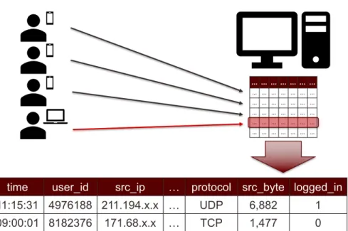
When we closer look at real-world datasets, they generally consist of different types of at-tributes including continuous, categorical, and binary atat-tributes. This is where one of the major difficulties of anomaly detection comes from: heterogeneous data. Figure 1.1 shows an example of heterogeneous data in computer networks.
In the example data, the features are of different types. For example, time, user_id, src_ip, and protocol are categorical features,src_byte is a continuous feature, and logged_inis a binary feature. Since each categorical feature can have different number of categorical values and all of the features are heterogeneous, it is really hard to measure the distance or similarity between two data instances. For example, what is the distance between the TCP and UDP protocols? Also, in streaming environments like computer network or credit card transaction example, the behaviors or distributions of data may change over time. What if a person living in Texas got a job in a different city of state and moved there? The pattern of credit card transactions of that person is going to totally change and credit card companies will get a lot of false alarms. In computer networks, attackers keep changing their behaviors so that they can prevent their anomalous behaviors from being detected by anomaly detection algorithms. This problem is also called concept drift and outlier detection algorithms for streaming data should be able to deal with this problem. Finally, it costs a lot of time and money to get the ground truth (labels) of data since we get very large amount of data everyday. Thus, we should assume that the ground truth of data is not available for anomaly detection tasks.
To tackle the aforementioned challenges, we propose an anomaly detection framework for heterogeneous and streaming data. Our strategies to deal with the challenges are motivated by previous work on anomaly detection. First of all, ensemble analysis has been overlooked for a long time because of the unsupervised nature of anomaly detection problems. By using an ensemble, we expect to achieve the diversity of detected outliers since each outlier detection algorithm reacts to categorical features differently. Also, we propose a distance metric for categorical features in order to make sure the ensemble model handles categorical features well. Second, outlier interpretation is very helpful for human experts to check whether detected outliers are really anomalous or not. Thus, we provide the interpretation of detected outliers to reduce the effort of human experts to get labels of data. Next, we enhance existing outlier detection methods so that they update their backend information regularly and can deal with concept drift issue. Finally, anomalies are not necessarily bad or malicious. Let me give you the credit card transaction example, again. In that
example, the credit card user just moved to other place, which is not a malicious activity, but just a less frequent activity. We do not want this kind of activities to be detected by our methods since these outliers increase false positives, which would cause the distrust on our framework. To address this problem, we use a supervised anomaly detection model along with the ensemble of unsupervised outlier detection methods.
Figure 1.2: The architecture of the proposed framework
The architecture of the proposed anomaly detection framework is illustrated in Figure 1.2. With these motivations, we build our framework having three phases. In the first phase, we detect suspi-cious records (outliers1) in streaming data by using an ensemble of two outlier detection methods. These methods are enhanced to update their backend information and deal with concept drift issue. We also introduce our own distance metric for categorical features so we can reasonably com-pute the distance between two heterogeneous data instances. In the second phase, the framework provides the interpretation of detected outliers in order to help human experts check whether the outliers are really anomalous or not and create the ground truth for the next phase. Finally, we
use a supervised anomaly detection model, which is a feed-forward neural network, and train this model using the ground truth from the previous phase to reduce false positives. Our feed-forward neural network has an embedding layer for categorical features in data to better deal with hetero-geneous data unlike other conventional supervised machine learning algorithms. This supervised model is simply used for binary classification tasks. Our framework has the following advantages over conventional anomaly detection methods:
• The framework can handle heterogeneous data by using an ensemble of outlier detection algorithms and our own distance metric for categorical attributes.
• The framework reduces the effort of human experts to classify anomalies by providing the outlier interpretation based on clusters and nearest neighbors.
• The framework can adapt to changing data behaviors in streaming data by updating its back-end information in real time.
• The framework reduces false positives as much as possible by using a supervised model and the feedback from human experts.
2. RELATED WORK
2.1 Anomaly Detection
A large number of studies on anomaly detection have been conducted, resulting in various techniques to address the problem. Scholkopfet al. [3] proposed Support Vector Machines with one-class setting for outlier detection. Some works try to detect outliers using density-based ap-proach [4, 5] and clustering-based method [6, 7, 8, 9]. Traditional nearest neighbor-based tech-niques have also been applied for outlier detection by [7, 10, 11]. Because of the characteristics of anomaly detection, some methods have been developed for specific purpose such as detecting outliers in attributed networks [12, 13].
With the recent success of neural networks, they have been used to capture anomalies in a unsupervised fashion. Hawkinset al. proposed Replicator Neural Networks (RNNs) for one-class anomaly detection and they are conceptually the same as autoencoders [14]. The RNNs try to learn input patterns and to reproduce them. The reconstruction error computed by subtracting the reconstructed output from an input instance is used as an anomaly score. Some recent works take advantage of deep architectures [15, 16, 17], showing that deep architectures can be used for unsupervised anomaly detection.
2.2 Heterogeneous Data
Not much of work on heterogeneous data exist since most of traditional outlier detection meth-ods focus on numerical attributes [1]. Otey et al. [18] proposed a distributed outlier detection method for heterogeneous and streaming data. This method captures dependencies among features of data so that they effectively compute the distance between two data points. The problem of this model is that it shows bad performance when data has only numerical attributes [18].
When it comes to categorical attributes, many existing models are probability based due to its discrete nature of data [19, 20]. One of interesting studies on categorial features is COMPREX pro-posed by Akogluet al.[21]. Anomalies are detected by this model if they have high compression
cost when compressing them. Chen et al. recently introduced a model addressing the problem of heterogeneous categorical data by finding pairwise interactions between categorical attributes using embeddings of them [22]. These models, however, can deal with only categorical attributes. 2.3 Streaming Data
Most studies on anomaly detection in streaming environments have been conducted in signal processing [23, 24, 25], which means they use only numerical data. The model introduced by Otey et al. [18] can deal with streaming data, but as we discussed above its performance deteriorates when using datasets with only numerical attributes. Tan et al. proposed Streaming Half-Space Trees in order to address the problem of concept drift and memory requirement [26], but the study solely focuses on numerical data like other traditional methods.
2.4 Ensemble Methods
Ensemble analysis has received considerable attention for supervised machine learning meth-ods due to its ability to boost a collection of algorithms. Following the trend, ensemble methmeth-ods for outlier detection also have been studied but in a limited way because of the unsupervised nature of the problem [27, 2].
One of the well-known ensemble methods for outlier detection is Local Outlier Factor (LOF) [4]. The LOF method computes LOF values within a range of values ofk, referring to the number of neighbors of a data instance. By taking the maximum of all the LOF values, they get an anomaly score for each instance. Isolation Forest proposed by [28] is an ensemble of isolation trees, which try to isolate each data instance from the rest of data instances. If a data point has a shorter path in a forest of such trees, then the point is highly likely to be anomalous. Recently, Chenet al.[29] introduced RandNet, employing autoencoder ensembles, to detect outliers. They could achieve the improved diversity and reduced training time by making autoencoders in RandNet have different structures and connection densities.
2.5 Interpretable Methods
The interpretation of outliers is important considering what we can benefit from it: interpre-tation (1) can help non-experts in a certain area look into results effectively and (2) reduce the effort of human experts and engineers analyzing results. Some works provide the interpretation of outliers by selecting features with which outlier detection methods find outliers most effec-tively [30, 31, 32]. There exist a general framework to explain classification results provided by any machine learning classifiers [33] and framework built for outlier interpretation [34].
2.6 Similarity Measures for Categorical Features
For measuring the distance or similarity between categorical attributes, the measure called the overlapmeasure [35] is the simplest and most widely used. In this measure, we just assign a value of 1 if two categorical values are same and assign a value of 0 if not. Although it does not depend on the ordering of categorical data, this measure is still too simplistic since it does not take into account other information which we can extract from categorical attributes such as the frequency information for each category.
By making use of these kinds of information, a lot of similarity or distance measure for cate-gorical data have been proposed. Eskin et al. introduced a data-dependent normalization kernel along with their anomaly detection algorithms in [7]. In this kernel, the distance between two categorical data is P 2
|fi|2 if two values offi are different, wherefi isi-th feature in data. This
kernel gives more weight to attributes that take small values when computing distances. The in-verse occurrence frequency derived from the inin-verse document frequency in information retrieval can also be used for a distance measure for categorical features. Each categorical value has a value oflog(f req(fi)N ), where N is the number of instances in data,f req(f)is the number of occurrences of the featuref in data, andfi isi-th feature in data. Other than these methods, probability-based
measures [36, 37, 38] and measures based on information theory [39, 40] have been proposed due to its discrete nature.
mea-sures for categorical data [41]. They revisited traditional techniques of the similarity meamea-sures for categorical data, proposed 6 variants of the existing methods, and perform experiments in the context of outlier detection. Their experiment results show that the performance of the similar-ity measures highly depends on datasets since different datasets have different characteristics of categorical attributes.
3. ANOMALY DETECTION FRAMEWORK
In this section, we propose an anomaly detection framework for heterogeneous and streaming data in order to tackle the challenges we discussed earlier: (1) heterogeneous data (2) concept drift issue in streaming data (3) no labeled data (4) not malicious anomalies. The framework has three phases to detect anomalies in streaming data and we explain each phase in detail as follows. The notations used in this paper are listed in Table 3.1.
Notation Definition
D training dataset xi a data instance
xij an attribute value ofxi
w the width of a cluster
k the number of nearest neighbors C a set of clusters
c a cluster∈C
d(xi, xj) the distance betweenxiandxj
df(xi, xj) the feature distance for the featuref
Kxi a set ofk-nearest neighbors ofxi
s(xi) the outlier score ofxi
Table 3.1: Notations used in the paper
3.1 Outlier Detection Methods
We selected two existing outlier detection algorithms from different outlier detection categories based on [1, 2]. The two selected methods are the Clustering Estimation (CE) and the k-Nearest Neighbor Approximation (kNNa) introduced by Eskinet al. [7]. The rationale behind selecting these two algorithms is, first of all, they are very simple and intuitive so we are able to provide the interpretation of results very easily. Second, they use the same backend information, which is the cluster information, so only one training is required for both methods. Furthermore, when
updating our backend information to deal with concept drift problem, we do not need to consider two different backend information for each method because we only have one backend information. Finally, they are computationally efficient so they are suitable for streaming data. We explain how each algorithm works and how we enhance them below.
3.1.1 Clustering Estimation
This method is also called fixed-width clustering [7]. It clusters data based on the fixed-width w of a cluster, which is a hyperparameter. The procedure of this algorithm is as follows. The method iterates all point in training data and it tries to find the closest cluster to each point. After finding the closest cluster to a point, the method checks if the point is within the closest cluster based on the fixed-widthw. If the point is within the closest cluster, then the point is added to the cluster. If not, the point will be the center of a new cluster. Formally we describe the procedure as: for each instancexi, xi is added to the closest cluster c∈C toxi ifd(xi, c)≤w. Ifd(xi, c)> w,
thenxi becomes the center of a new cluster. Algorithm 1 illustrates the pseudocode for the CE.
Algorithm 1:Clustering Estimation algorithm
1 LetCbe an empty set;
2 foreach record in training datado
3 Find the closest clustercto the current recordxi; 4 ifd(xi,c)≤wthen 5 c:=c∪ {xi}; 6 else 7 makeNewCluster(C,xi); 8 end 9 end 10 returnC
The time complexity of this method for clustering (training) isO(n|C|), wherenis the number of instances in a given training datasetD. Since the number of clusters is typically much less than the number of instances in training data, we can cluster training data very efficiently. The outlier
scores(xi)for a new instancexi is the inverse of the size of the closest cluster toxi ifxi is within
the clustercand is formally defined as:
s(xi) = 1 |c|, ifd(xi, c)≤w 1, otherwise (3.1)
where w is the predefined cluster width, c is the closest cluster to xi and c∈ C, which is a set
of clusters. For outlier detection, we train the model with training data, which means that we get clustersCbased on the training dataset. After training, we evaluate a new instancexiin streaming
data by finding the closest cluster cto xi and computing the outlier score of xi. Computing the
outlier score of an instance takesO(|C|)time since we find the closest cluster to the instance. The higher score an instance has, the more outlying it is.
3.1.2 k-Nearest Neighbor Approximation
As the name of the method suggests, it findsk-nearest neighbors of an instance to detect anoma-lies. We modified the original algorithm in [7] to make it more simple and efficient. Here is how it works. First of all, we apply the Clustering Estimation algorithm to get our backend cluster in-formationC. We find the closest clustercto a new instancexi from streaming data, which means
that we computeargminc∈C d(xi, c), and then add all instances incto a setKxi if|c| ≤k-|Kxi|.
After that, we find the second closest cluster and do the same process. If the condition is not met, then randomly pick k -|Kxi|number of instances incand add them toKxi. Algorithm 2 shows
the pseudocode for thekNNa.
The time complexity of this method for training is the same as that of the CE since the training process is the same and it only takesO(|C|)when findingk-nearest neighbors for a single instance. The outlier score s(xi) for a new instance xi is the sum of the distances between xi and each
instance inKxi and is formally defined as:
s(xi) =
X
y∈Kxi
Algorithm 2:k-Nearest Neighbor Approximation algorithm
1 LetCbe the result of the CE algorithm; 2 LetCcheckedbe an empty set;
3 Letxibe a new instance from streaming data; 4 LetKxi be an empty set;
5 while|Kxi|<k do
6 Find the closest clusterc∈C-Ccheckedtoxi; 7 if|Kxi|+|c| ≤kthen
8 Kxi :=Kxi ∪ {all points∈c};
9 else
10 P :=k-|Kxi|points picked fromcat random;
11 Kxi :=Kxi ∪P;
12 end
13 Cchecked:=Cchecked∪ {c} 14 end
15 returnKxi
For outlier detection, we train the model with training data by using the CE to get clustersC. After that, we find k-nearest neighbors of a new instance xi in streaming data using this method and
compute the outlier score ofxi. The higher score an instance has, the more outlying it is.
3.2 Update Backend Information
To deal with concept drift, we update our backend cluster information by adopting the idea used for the Streaming HS trees [26]. The Steaming HS trees maintain two separate backend information. At first, one called reference window is created using training data and the other calledlatest window is created using streaming data (latest data). Thereference window is used for classification task when they get a new data instance and they save this instance to thelatest window for future use. After getting enough information about streaming data, they replace the referencewindow with thelatestwindow. By doing so, they can adapt to changing data behaviors in streaming environments.
Thanks to the characteristic of the clustering algorithm that we use, we can adopt this idea. As a new data instance arrives, we can apply the CE method to cluster streaming data. This process takes
onlyO(|C|)time, where|C| is the number of clusters, so we can efficiently do this in streaming environments. At the same time, we do the classification task for the new data instance by using our original backend information based on training data. The classification task also takesO(|C|)
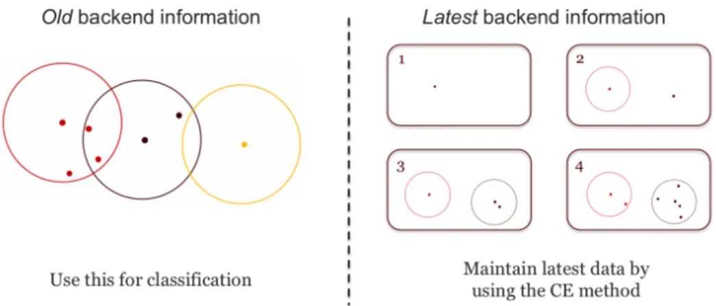
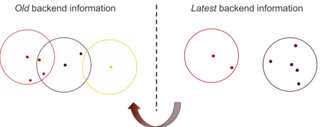
time as we discussed in the earlier sections. Thus, we are able to not only classify a new data instance but also use it for clustering in streaming environments. Figure 3.1 and 3.2 illustrate how this process works.
Figure 3.1: Two separate backend information; we use theoldbackend information for classifica-tion tasks and apply the CE method to save latest data informaclassifica-tion.
We have two separate backend cluster information as the Streaming HS trees do: one that we call oldbackend information based on training data and the other that we calllatestbackend information based on streaming data. When we get a new data instance, the outlier score of the new instance is computed using the old backend information based on training data. With the new data instance, we also apply the CE method to the latestbackend information for clustering task. We keep doing this process until the number of instances in the latest backend reaches a predefined threshold. After that point, we replace the old backend information with the latest backend information. By doing so, we expect to deal with concept drift issue.
Figure 3.2: Replacement of the backend information; when the number of instances in thelatest backend exceeds a predefined threshold, we replace theoldbackend with thelatestone.
3.3 Distance Metric for Categorical Attributes
It is hard to compute the distance between two categorical instances since categorical data cannot be ordered in most cases. For example, we cannot say that udpis greater thattcp orhttp is less than smtp. Due to this issue, we usually apply one-hot encoding where each category is translated to an one-hot vector corresponding its categorical value or use Hamming distance, which is the number of categories which have different categorical values between two instances. However, these techniques do not take into account the data distribution so it is unlikely that these are helpful for anomaly detection tasks. Table 3.2 shows an example of categorical values and their frequencies ofprotocol_type andservice categories.
According to a survey on similarity measure for categorical data, introduced by Boriah et al. [41], we cannot choose a single measure as the best one for categorical data since the per-formance of similarity and distance measure depends on datasets. However, some of them show consistently better performance on the benchmark datasets that they used and they are in com-mon in terms of the use of the frequency information for each category. They give higher weight on infrequent values if two values are different. We intend to adopt this concept along with the data-dependent normalization kernel proposed in [7] to introduce a new distance metric for our
protocol_type service
Value Frequency Value Frequency
tcp 20,526 http 8,003 private 4,351 udp 3,011 smtp 1,449 ftp_data 1,396 icmp 1,655 telnet 483 other 1,944
Table 3.2: Categorical values and their frequencies ofprotocol_type andservice categories
framework.
The first thing we need to consider is the number of possible categorical values for each cat-egory, which is called arity. The reason is that the importance of the value difference between a category having 3 possible values and a category having 6 possible values should be differenti-ated. Let me take an example of Table 3.2. The value difference ofprotocol_type should be more weighted than that of service because the value difference of attributes that take many values is more like a marginal difference than that of attributes that take small number of values.
Second, we also need to consider the frequency of each categorical value since in outlier detec-tion tasks the less frequent value is considered anomalous. In Table 3.2, for example, the distance between “http” and “smtp” should be greater than that between “smtp” and “ftp_data” considering the frequency gap. With these in mind, we define the distanced(xi, xj)and the feature distance
df(xi, xj)betweenxi andxj as follows:
dfcat(xi, xj) =
log(1+|f req(fxi)−f req(fxj)|)
arity(f) , iffxi 6=fxj
0, otherwise
(3.3)
df(xi, xj) = dfcat(xi, xj), iff ∈Fcat dfnum(xi, xj), iff ∈Fnum (3.5) d(xi, xj) = s X f∈F df(xi, xj) (3.6)
where F is a set of attributes of data, Fcat is a set of categorical features ∈F, Fnum is a set
of numerical features ∈ F, f is an attribute ∈ F, fxi is an attribute value of xi for the attribute
f, f req(fxi) is the number of occurrences offxi in training data, andartiy(f)is the number of
possible attribute values of the feature f. By using these distance metrics, we can compute the distance between <tcp, http> and <udp, private> as log(1 + |20,526 −3,011|)/3 + log(1 +
|8,003−4,351|)/6equal to 4.6242, which ls greater than the distance between<tcp, smtp>and <udp, ftp_data>equal to 3.9218.
3.4 Outlier Ensembles
Ensemble methods in outlier detection areas have not been studied very well due to the fact that the ground truth of data is not available [27, 2]. Because of this constraint, we are not able to adopt ensemble techniques used in supervised settings such as boosting. In order to achieve the diversity of detected outliers and higher performance of our framework, we intend to combine the afore-mentioned outlier detection methods altogether. Since all of these algorithms are unsupervised and different types of models, it is hard to combine outlier scores provided by them. We have two major issues for the ensemble process according to [27, 2], normalization and combination issues. The normalization issues arise from the fact that outlier scores from different methods cannot be directly compared since different algorithms use different scales of outlier scores. For example an outlier score from the CE method is computed based on a cluster size, but an outlier score from the kNNa is computed based on the nearest neighbors of a detected outlier. Outlier scores from CE ranges from 0 to 1, but those from thekNNa ranges from 0 to some number that we do not
know. Normalizing these scores could solve this issue, but streaming data make this worse since it is difficult to normalize outlier scores in streaming data environments.
Even if we can normalize these scores, all of the scores should be combined in some ways after the normalization process. How we combine these scores also affects the performance of the ensemble, which makes this problem difficult. To avoid these issues, we use the majority voting ensemble by setting a score threshold for each outlier detection method. In majority voting, each method classifies a new data instance and the majority opinion of the methods that we have would be our classification result. Since our framework has only two outlier detection methods, a new data instance is classified as an anomaly if both methods agree on that. The framework is a general framework where users can add their custom outlier detection methods to the ensemble. Thus, if users added their custom model to the ensemble, then a classification result would be made based on the result of the majority of the methods. Furthermore, the framework provides the confidence that represents the result of a majority voting. For example, if 4 methods out of 5 agree that a new instance is an anomaly, then the new instance would be classified as an anomaly with the confidence of 80%.
3.5 Classification By Human Experts With Outlier Interpretation
In Phase 2, human experts check whether detected outliers in the previous phase are really anomalous or not. In order to facilitate this work, we provide the interpretation of detected outliers based on clusters and nearest neighbors information. What we would like in this phase is to provide the interpretation of a new instance as soon as we classify it since the framework is working in streaming environments. Due to this constraint, we are not able to use the existing interpretation methods for the framework. Now, we introduce our interpretation method for streaming data. 3.5.1 Interpretation of Outliers
Our strategy is to find features that make detected outliers anomalous, which is a traditional approach for machine learning interpretation [30, 31, 32]. Since we have the cluster information of training data and nearest neighbors of detected outliers, we utilize this information to achieve
the interpretation of detected outliers. We define the feature importance score of each feature for a detected outlierobased on our backend cluster information andk-nearest neighbors ofoas follows.
sf(o) = X c∈C |c|df(o, c) + X y∈Ko df(o, y) (3.7)
whereKo is a set of nearest neighbors of a detected outliero and y is an instance ∈Ko. The
first term is computed based on the cluster information and the nearest neighbors of o are used to compute the second term. The intuition behind these terms is that (1) the smaller clusters, the more anomalous and (2) the nearest neighbors of o are the most relevant information of it becauseo is classified as an outlier based on them. Thus, we give more weights to large clusters using the size of clusters so that points in large clusters (i.e., normal clusters) have more impact on computing the feature importance score. If some attribute value of o is different from that of points in large clusters, then the feature importance score of that attribute would be high. Also, the nearest neighbors ofoare used to classify a detected outlieroso we already know the nearest neighbors of it. Because of this fact, we can save time to find the nearest neighbors of a detected outlier. With the nearest neighbors ofo, we compute the feature importance score by summing up the feature distance between o and each instance of its nearest neighbors for each attribute. We can think of the first term in Equation 3.7 as theglobalinterpretation because we basically use all of information in training data. On the other hand, we can think of the second term as thelocal interpretation since the nearest neighbors ofo are the local information of detected outliers. By incorporating the local information (i.e., nearest neighbor information) with the global information (i.e., cluster information), we expect to provide reasonable interpretations of detected outliers.
With the help of outlier interpretation, human experts could identify “actual” anomalies in de-tected outliers more easily. After the classification tasks by human experts, they provide a feedback (i.e., ground truth) containing abnormal instances to the next phase. The rest of the data that are not classified as anomalies are considered normal.
3.6 Supervised Anomaly Detection
Outliers are obviously different from normal instances but they might not be bad or malicious. In order to distinguish not-malicious outliers from malicious outliers, we use a supervised anomaly detection approach in Phase 3. For this task, a feed-forward neural network is used. Figure 3.3 shows the architecture of the feed-forward neural network used in our framework.
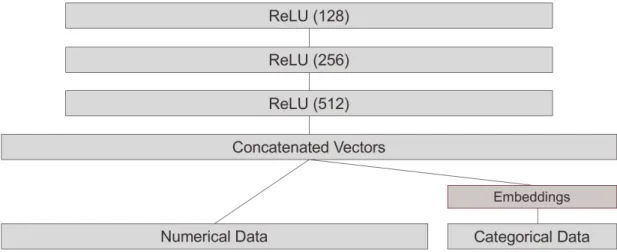
Figure 3.3: The architecture of a neural network used in Phase 3
The neural network has a embedding layer to better deal with categorical data, but numerical data are directly used. After the embedding layer, we concatenate numerical data and embeddings for categorical data. On top of concatenated vectors, we have three ReLU layers. As for the output layer, the sigmoid function is used as the activation function. The model can be replaced with traditional supervised machine learning algorithms, but they should be able to handle both heterogeneous and streaming data. For example, a logistic regression model may not be suitable for this task since the model cannot deal with heterogeneous data.
The procedure of this phase is as follows. First, we get the feedback from human experts in Phase 2. With the feedback, we train our supervised model. If the amount of data in the feedback is not enough, we wait for another feedback and accumulate the feedbacks so that we can train
the model properly. Our ultimate goal is to skip the first and second phase and just to use the supervised model for anomaly detection tasks. Users of the framework may continue to use the first two phases when too many false positives occur due to concept drift or other reasons.
4. EXPERIMENTS
By performing experiments on real world datasets, we show the efficacy of our proposed frame-work. We would like to answer the following questions in this section: (1) Can the framework deal with heterogeneous data? (2) Can the framework handle concept drift? (3) Are interpretation re-sults reliable? (4) Can the framework reduce false positives? To answer the first question, we evaluate our ensemble model by using two types of datasets: one with only numerical features and the other with all features. For the evaluation on streaming data, we follow the experiment setup in [26] to simulate changing data behaviors. We show some examples of the interpretation results of detected outliers for the evaluation on outlier interpretation. Finally, we simulate each phase in the framework to evaluate the whole framework.
4.1 Dataset
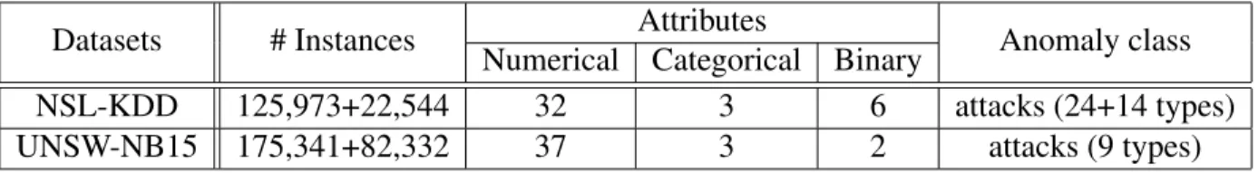
For our experiments, we use two network intrusion detection datasets: NSL-KDD [42] and UNSW-NB15 [43]. The NSL-KDD dataset is introduced to improve problems that the KDD-CUP99 dataset [44] originally has such as a lot of redundant instances. It has 24 types of attacks in the training set and additional 14 types of attacks in the test set, which are not available in the training set. The UNSW-NB15 contains 9 types of attacks in both the training and test sets. Both datasets have real normal activities along with synthetic attack behaviors and consist of different types of attributes. Table 4.1 illustrates the details of the datasets.
Datasets # Instances Attributes Anomaly class
Numerical Categorical Binary
NSL-KDD 125,973+22,544 32 3 6 attacks (24+14 types)
UNSW-NB15 175,341+82,332 37 3 2 attacks (9 types)
We do not use the cross-validation technique, but only use the given training and test sets. This is because the datasets are very sensitive to the number of attacks and types of attacks in training and test sets. The datasets are designed considering these issues and we would not be able to measure the performances of our framework and a baseline method If we use the cross-validation technique.
4.2 Experiment Setup
We randomly removed most of abnormal instances in the training data so that they contain about 1% of anomalies and 99% of normal instances, which is a more realistic setting than the original datasets. Even though the ground truth labels of the datasets are available, they are not used during training the ensemble model in Phase 1, but used solely for evaluation. As our baseline, we use Isolation Forest [28], which is one of the state of the art outlier detection methods. The Isolation Forest consists of isolation trees, which try to isolate each data instance from the rest of the data. Since outliers are different and a few, it is easier to isolate outliers than normal instances. Therefore, if an instance has shorter path length in isolation trees, then it is likely to be an outlier. Since the Isolation Forest is not designed for streaming data, we expect that the model shows bad performance in our simulated streaming environment.
As for the preprocessing of data, we standardize numerical attributes in our training data. Based on the mean and standard deviation of the training data, an incoming instance in streaming data is standardized. Categorical attributes are handled with our distance metric that we introduced in this paper. The mean and standard deviation information are updated when the backend information of the framework is updated.
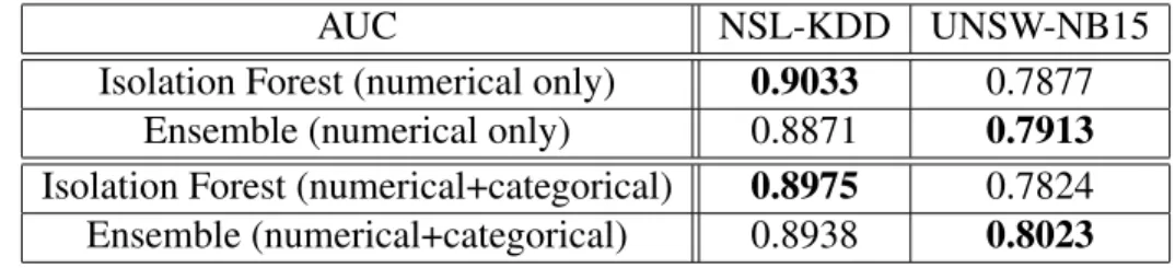
4.3 Evaluation on Heterogeneous Data
In this experiment, we evaluate the ability of our framework to deal with heterogeneous data. Two types of datasets are used to see if the framework and the baseline can handle heterogeneous data well: one with only numerical features and the other with all features. We expect that if one can deal with heterogeneous data well, then the performance would increase. Table 4.2 shows the
experiment results and AUC (Area Under Curve) values are reported as the evaluation metric.
AUC NSL-KDD UNSW-NB15
Isolation Forest (numerical only) 0.9033 0.7877
Ensemble (numerical only) 0.8871 0.7913
Isolation Forest (numerical+categorical) 0.8975 0.7824 Ensemble (numerical+categorical) 0.8938 0.8023
Table 4.2: Experiment results on static heterogeneous datasets
The ensemble model could show comparable performance with the baseline on NSL-KDD dataset in both cases where the dataset has only numerical attributes and all features. However, the performance of the Isolation Forest deteriorates when categorical attributes are added to the dataset, but the performance of the ensemble model increases as we expected. On the UNSW-NB15 dataset, the ensemble model constantly outperforms the baseline method and the perfor-mance of the ensemble increases when categorical features are used along with numerical features. However, the baseline on the dataset with only numerical features shows slightly worse perfor-mance than on the dataset with all features. The experiment results are consistent with our expec-tation that it can deal with heterogeneous data as the ensemble model shows better performance on the datasets with all features.
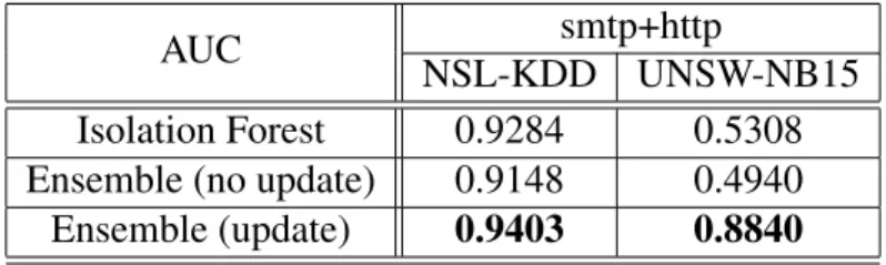
4.4 Evaluation on Streaming Data
In order to evaluate the ability of our framework to handle the concept drift issue, we simulate changing data behaviors by following the experiment setup in [26]; we train our ensemble model using data only withsmtp protocol, and then test the ensemble model using data withsmtp pro-tocol followed by http protocol. As the network protocol changes in the dataset, we expect the concept drift would occur. Table 4.3 shows the experiment results and AUC values are reported as the evaluation metric.
AUC smtp+http
NSL-KDD UNSW-NB15
Isolation Forest 0.9284 0.5308 Ensemble (no update) 0.9148 0.4940
Ensemble (update) 0.9403 0.8840
Table 4.3: Experiment results on streaming datasets
on the NSL-KDD dataset. We speculate that the protocol change was not able to change data distributions using the NSL-KDD dataset. However, the ensemble with updating shows the best performance over the other models. On the UNSW-NB15 dataset, the ensemble model with up-dating performs really well, but the others show very bad performance as we expected. It shows that the ensemble with updating could adapt to changing data distributions and the other models are not able to deal with the concept drift since they are originally designed to detect anomalies in static datasets.
4.5 Evaluation on Outlier Interpretation
To verify that our interpretation of detected outliers are reliable, we show the interpretation results for both normal and abnormal instances in Figure 4.1, 4.2,and 4.3. In the bar graphs showing the feature importance scores, y-axis represents the feature importance score for each attribute and x-axis represents attributes in data.
As you see the bar graphs in Figure 4.1, the feature importance scores are almost uniformly distributed over features compared to the bar graphs of abnormal instances in Figure 4.2 and 4.3 since normal instances do not have specific anomalous attributes. Most of the feature importance scores of abnormal instances are very low and a few of them stand out. We could find the first and second most anomalous attributes based on the scores at the top in Figure 4.2 and 4.3 and further analyze the results by using scatter plots. In each scatter plot, there is a red point marked with a red circle and it represents a detected outlier used in each example. In Figure 4.2 example, the two anomalous attributes are srv_count andsrv_rerror_rate and data instances are shown using
these two attributes at the bottom of the figure. As you see the scatter plot, we are, indeed, able to distinguish most of abnormal instances from normal instances by using only these two attributes. In Figure 4.3 example, the two anomalous attributes aredst_bytesandnum_compromisedand data instances are shown using these two attributes at the bottom of the figure as we did above. Unlike the previous example, we are able to distinguish all of abnormal instances from normal instances by using only these two attributes as you see the scatter plot.
4.6 Framework Evaluation
The purpose of this experiment is to evaluate the whole framework. For this experiment, we divide the test dataset into 5 batches. After that, we detect outliers in a single batch and a feedback is created based on the ground truth to simulate the classification by human experts. Our supervised model is trained with the feedback and tested with the last batch (fifth batch), which is only used for evaluating the supervised model. We keep doing this process until the 4th batch. In summary, we detect suspicious records (i.e., outliers) in the first 4 batches in turn, and then we train the supervised model with the feedback from each batch. In this experiment, we report the values of precision, recall, andF1 score shown in Table 4.4.
Batch NSL-KDD UNSW-NB15
Precision Recall F1 Precision Recall F1
1st Batch Ensemble 0.89 0.73 0.80 0.76 0.70 0.73 Supervised 0.89 0.75 0.82 0.98 0.65 0.78 2nd Batch Ensemble 0.90 0.73 0.81 0.77 0.69 0.73 Supervised 0.91 0.78 0.84 0.97 0.67 0.79 3rd Batch Ensemble 0.89 0.72 0.80 0.78 0.71 0.74 Supervised 0.92 0.79 0.85 0.96 0.71 0.82 4th Batch Ensemble 0.90 0.74 0.81 0.77 0.70 0.73 Supervised 0.94 0.79 0.85 0.97 0.73 0.83
Table 4.4: Experiment results for the supervised model in Phase 3
batch is used to provide the result of the ensemble on the first batch. However, the result of the supervised model is provided based on the last batch (the fifth batch). As you see the table, the results of the ensemble are consistent over the batches, so we could tell the ensemble is stable to detect outliers. As for the supervised model, the performance gets better as we accumulate the feedbacks. We would like to remind you that the reason why we use the supervised model in the last phase is to reduce false positives, especially from outliers that are different from normal instances but not malicious. The precision values increase without the decrease of the recall values on the NSL-KDD dataset. Even though the precision values decrease by 0.01 to 0.02 as we get more feedbacks, the F1 values increase on the UNSW-NB15 dataset. You may notice that the
precision values on the UNSW-NB15 dataset are higher than those on the NSL-KDD dataset. We speculate that this may arise from the fact that the UNSW-NB15 dataset has less number of attack types so there is a chance that the supervised model is overfitted to some attack patterns. Overall, these results are consistent with our expectation that the supervised model could take advantage of accumulated feedbacks.
Figure 4.1: Examples of the interpretation results on the NSL-KDD dataset; the bar graphs show the feature importance scores for each attribute of normal instances. As you see the figures, the scores are well distributed over features. This is because normal instances do not have specific anomalous attributes.
Figure 4.2: Examples of the interpretation results on the NSL-KDD dataset; the top figure shows the feature importance scores for each attribute of a detected outlier, and the bottom figure shows a scatter plot of the first and second most anomalous attributes,srv_countandsrv_rerror_ratebased on the feature importance scores. In the scatter plot, red points represent abnormal instances, and blue points represent normal instances. The red point marked with the red circle refers to the detected outlier.
Figure 4.3: Examples of the interpretation results on the NSL-KDD dataset; the top figure shows the feature importance scores for each attribute of a detected outlier, and the bottom figure shows a scatter plot of the first and second most anomalous attributes,dst_bytesandnum_compromised based on the feature importance scores. In the scatter plot, red points represent abnormal instances, and blue points represent normal instances. The red point marked with the red circle refers to the detected outlier.
5. CONCLUSION AND FUTURE WORK
In this paper, we propose an anomaly detection framework for heterogeneous and streaming data. The framework was able to handle heterogeneous data and achieve comparable performance with the state of the art baseline method on the network intrusion detection datasets using an en-semble of two outlier detection algorithms and our distance metric for categorical attributes. These methods are enhanced to update the backend cluster information so that they could adapt to chang-ing data behaviors (concept drift). In the second phase of the framework, outlier interpretation is provided to help human experts to check whether detected outliers are really anomalous and we have shown that interpretation results are reasonable, giving the interpretation examples. Fi-nally, the supervised machine learning algorithm was trained with the feedbacks from Phase 2 and successfully reduced false positives with accumulated anomaly information.
The work can be extended by trying parameter optimization techniques based on the predefined contamination ratio (outlier ratio) since we have a score threshold for each method to tune. Using different supervised models which can handle heterogeneous and streaming data such as Hoeffding Trees [45] and Wide & Deep Learning model [46] might help the framework. Finally, it would be very helpful to analyze detected outliers and the interpretation of them if we had the graphical interface of the framework.
REFERENCES
[1] V. Chandola, A. Banerjee, and V. Kumar, “Anomaly detection: A survey,” ACM computing surveys (CSUR), vol. 41, no. 3, p. 15, 2009.
[2] C. C. Aggarwal, “Outlier analysis,” inData mining, pp. 237–263, Springer, 2015.
[3] B. Schölkopf, R. C. Williamson, A. J. Smola, J. Shawe-Taylor, and J. C. Platt, “Support vector method for novelty detection,” inAdvances in neural information processing systems, pp. 582–588, 2000.
[4] M. M. Breunig, H.-P. Kriegel, R. T. Ng, and J. Sander, “Lof: identifying density-based local outliers,” inACM sigmod record, vol. 29, pp. 93–104, ACM, 2000.
[5] J. Tang, Z. Chen, A. Fu, and D. Cheung, “Enhancing effectiveness of outlier detections for low density patterns,” Advances in Knowledge Discovery and Data Mining, pp. 535–548, 2002.
[6] L. Portnoy, E. Eskin, and S. Stolfo, “Intrusion detection with unlabeled data using clustering,” inIn Proceedings of ACM CSS Workshop on Data Mining Applied to Security (DMSA-2001, Citeseer, 2001.
[7] E. Eskin, A. Arnold, M. Prerau, L. Portnoy, and S. Stolfo, “A geometric framework for un-supervised anomaly detection: Detecting intrusions in unlabeled data,”Applications of data mining in computer security, vol. 6, pp. 77–102, 2002.
[8] P. K. Chan, M. V. Mahoney, and M. H. Arshad, “A machine learning approach to anomaly detection,” tech. rep., 2003.
[9] Z. He, X. Xu, and S. Deng, “Discovering cluster-based local outliers,” Pattern Recognition Letters, vol. 24, no. 9, pp. 1641–1650, 2003.
[10] F. Angiulli and C. Pizzuti, “Fast outlier detection in high dimensional spaces,” inEuropean Conference on Principles of Data Mining and Knowledge Discovery, pp. 15–27, Springer, 2002.
[11] J. Zhang and H. Wang, “Detecting outlying subspaces for high-dimensional data: the new task, algorithms, and performance,” Knowledge and information systems, vol. 10, no. 3, pp. 333–355, 2006.
[12] N. Liu, X. Huang, and X. Hu, “Accelerated local anomaly detection via resolving attributed networks,”
[13] J. Li, H. Dani, X. Hu, and H. Liu, “Radar: Residual analysis for anomaly detection in at-tributed networks,”IJCAI?17, 2017.
[14] S. Hawkins, H. He, G. Williams, and R. Baxter, “Outlier detection using replicator neural networks,” inDaWaK, vol. 2454, pp. 170–180, Springer, 2002.
[15] S. Zhai, Y. Cheng, W. Lu, and Z. Zhang, “Deep structured energy based models for anomaly detection,” inInternational Conference on Machine Learning, pp. 1100–1109, 2016.
[16] C. Zhou and R. C. Paffenroth, “Anomaly detection with robust deep autoencoders,” in Pro-ceedings of the 23rd ACM SIGKDD International Conference on Knowledge Discovery and Data Mining, pp. 665–674, ACM, 2017.
[17] B. Zong, Q. Song, M. R. Min, W. Cheng, C. Lumezanu, D. Cho, and H. Chen, “Deep autoen-coding gaussian mixture model for unsupervised anomaly detection,” 2018.
[18] M. E. Otey, A. Ghoting, and S. Parthasarathy, “Fast distributed outlier detection in mixed-attribute data sets,” Data mining and knowledge discovery, vol. 12, no. 2-3, pp. 203–228, 2006.
[19] K. Das and J. Schneider, “Detecting anomalous records in categorical datasets,” in Proceed-ings of the 13th ACM SIGKDD international conference on Knowledge discovery and data mining, pp. 220–229, ACM, 2007.
[20] K. Das, J. Schneider, and D. B. Neill, “Anomaly pattern detection in categorical datasets,” inProceedings of the 14th ACM SIGKDD international conference on Knowledge discovery and data mining, pp. 169–176, ACM, 2008.
[21] L. Akoglu, H. Tong, J. Vreeken, and C. Faloutsos, “Fast and reliable anomaly detection in categorical data,” inProceedings of the 21st ACM international conference on Information and knowledge management, pp. 415–424, ACM, 2012.
[22] T. Chen, L.-A. Tang, Y. Sun, Z. Chen, and K. Zhang, “Entity embedding-based anomaly detection for heterogeneous categorical events,” inProceedings of the Twenty-Fifth Interna-tional Joint Conference on Artificial Intelligence, pp. 1396–1403, 2016.
[23] R. M. Tallam, T. G. Habetler, and R. G. Harley, “Self-commissioning training algorithms for neural networks with applications to electric machine fault diagnostics,”IEEE Transactions on Power Electronics, vol. 17, no. 6, pp. 1089–1095, 2002.
[24] M. Davy, F. Desobry, A. Gretton, and C. Doncarli, “An online support vector machine for abnormal events detection,”Signal processing, vol. 86, no. 8, pp. 2009–2025, 2006.
[25] S. Subramaniam, T. Palpanas, D. Papadopoulos, V. Kalogeraki, and D. Gunopulos, “Online outlier detection in sensor data using non-parametric models,” in Proceedings of the 32nd international conference on Very large data bases, pp. 187–198, VLDB Endowment, 2006. [26] S. C. Tan, K. M. Ting, and T. F. Liu, “Fast anomaly detection for streaming data,” inIJCAI
Proceedings-International Joint Conference on Artificial Intelligence, vol. 22, p. 1511, 2011. [27] C. C. Aggarwal, “Outlier ensembles: position paper,”ACM SIGKDD Explorations
Newslet-ter, vol. 14, no. 2, pp. 49–58, 2013.
[28] F. T. Liu, K. M. Ting, and Z.-H. Zhou, “Isolation forest,” inData Mining, 2008. ICDM’08. Eighth IEEE International Conference on, pp. 413–422, IEEE, 2008.
[29] J. Chen, S. Sathe, C. Aggarwal, and D. Turaga, “Outlier detection with autoencoder ensem-bles,” inProceedings of the 2017 SIAM International Conference on Data Mining, pp. 90–98, SIAM, 2017.
[30] E. M. Knorr and R. T. Ng, “Finding intensional knowledge of distance-based outliers,” in VLDB, vol. 99, pp. 211–222, 1999.
[31] B. Micenková, X.-H. Dang, I. Assent, and R. T. Ng, “Explaining outliers by subspace separa-bility,” inData Mining (ICDM), 2013 IEEE 13th International Conference on, pp. 518–527, IEEE, 2013.
[32] N. X. Vinh, J. Chan, S. Romano, J. Bailey, C. Leckie, K. Ramamohanarao, and J. Pei, “Dis-covering outlying aspects in large datasets,”Data Mining and Knowledge Discovery, vol. 30, no. 6, pp. 1520–1555, 2016.
[33] M. T. Ribeiro, S. Singh, and C. Guestrin, “Why should i trust you?: Explaining the predictions of any classifier,” in Proceedings of the 22nd ACM SIGKDD International Conference on Knowledge Discovery and Data Mining, pp. 1135–1144, ACM, 2016.
[34] N. Liu, D. Shin, and X. Hu, “Contextual outlier interpretation,” inProceedings of the Twenty-Seventh International Joint Conference on Artificial Intelligence, 2018.
[35] C. Stanfill and D. Waltz, “Toward memory-based reasoning,”Communications of the ACM, vol. 29, no. 12, pp. 1213–1228, 1986.
[36] D. W. Goodall, “A new similarity index based on probability,”Biometrics, pp. 882–907, 1966. [37] E. Smirnov, “On exact methods in systematics,”Systematic Biology, vol. 17, no. 1, pp. 1–13,
1968.
[38] M. R. Anderberg, “Cluster analysis for applications,” tech. rep., Office of the Assistant for Study Support Kirtland AFB N MEX, 1973.
[39] D. Linet al., “An information-theoretic definition of similarity.,” inIcml, vol. 98, pp. 296– 304, Citeseer, 1998.
[40] T. Burnaby, “On a method for character weighting a similarity coefficient, employing the concept of information,”Journal of the International Association for Mathematical Geology, vol. 2, no. 1, pp. 25–38, 1970.
[41] S. Boriah, V. Chandola, and V. Kumar, “Similarity measures for categorical data: A compara-tive evaluation,” inProceedings of the 2008 SIAM International Conference on Data Mining, pp. 243–254, SIAM, 2008.
[42] M. Tavallaee, E. Bagheri, W. Lu, and A. A. Ghorbani, “A detailed analysis of the kdd cup 99 data set,” inComputational Intelligence for Security and Defense Applications, 2009. CISDA 2009. IEEE Symposium on, pp. 1–6, IEEE, 2009.
[43] N. Moustafa and J. Slay, “Unsw-nb15: a comprehensive data set for network intrusion de-tection systems (unsw-nb15 network data set),” inMilitary Communications and Information Systems Conference (MilCIS), 2015, pp. 1–6, IEEE, 2015.
[44] D. Dheeru and E. Karra Taniskidou, “UCI machine learning repository,” 2017.
[45] P. Domingos and G. Hulten, “Mining high-speed data streams,” inProceedings of the sixth ACM SIGKDD international conference on Knowledge discovery and data mining, pp. 71– 80, ACM, 2000.
[46] H.-T. Cheng, L. Koc, J. Harmsen, T. Shaked, T. Chandra, H. Aradhye, G. Anderson, G. Cor-rado, W. Chai, M. Ispir, et al., “Wide & deep learning for recommender systems,” in Pro-ceedings of the 1st Workshop on Deep Learning for Recommender Systems, pp. 7–10, ACM, 2016.