Advancing Pancreas Segmentation in Multi-protocol MRI Volumes using Hausdorff-Sine Loss Function

WestminsterResearch

http://www.westminster.ac.uk/westminsterresearch

Advancing Pancreas Segmentation in Multi-protocol MRI

Volumes using Hausdorff-Sine Loss Function

Asaturyan, H., Thomas, E.L., Fitzpatrick, J., Bell, J.D. and Villarini,

B.

This is an author's accepted manuscript of an article published in the proceedings of the

10th International Workshop on Machine Learning in Medical Imaging (MLMI 2019) in

conjunction with MICCAI 2019. Shenzen, China 13 Oct 2019 Springer.

doi:10.1007/978-3-030-32692-0_4 .

The final authenticated publication is available at Springer via:

https://dx.doi.org/10.1007/978-3-030-32692-0_4

The WestminsterResearch online digital archive at the University of Westminster aims to make the research output of the University available to a wider audience. Copyright and Moral Rights remain with the authors and/or copyright owners.

Whilst further distribution of specific materials from within this archive is forbidden, you may freely distribute the URL of WestminsterResearch: ((http://westminsterresearch.wmin.ac.uk/).

Multi-protocol MRI Volumes using

Hausdorff-Sine Loss Function

Hykoush Asaturyan1[0000−0002−7251−9464], E. Louise Thomas2, Julie Fitzpatrick2, Jimmy D. Bell2, and Barbara Villarini1

1

University of Westminster, School of Computer Science and Engineering, London, United Kingdom

[email protected], [email protected]

2 _{University of Westminster, School of Life Sciences, London, United Kingdom}

{L.Thomas3,J.Fitzpatrick,J.Bell}@westminster.ac.uk

Abstract. Computing pancreatic morphology in 3D radiological scans

could provide significant insight about a medical condition. However, segmenting the pancreas in magnetic resonance imaging (MRI) remains challenging due to high inter-patient variability. Also, the resolution and speed of MRI scanning present artefacts that blur the pancreas bound-aries between overlapping anatomical structures. This paper proposes a dual-stage automatic segmentation method: 1) a deep neural network is trained to address the problem of vague organ boundaries in high class-imbalanced data. This network integrates a novel loss function to rigorously optimise boundary delineation using the modified Hausdorff metric and a sinusoidal component; 2) Given a test MRI volume, the output of the trained network predicts a sequence of targeted 2D pan-creas classes that are reconstructed as a volumetric binary mask. An energy-minimisation approach fuses a learned digital contrast model to suppress the intensities of non-pancreas classes, which, combined with the binary volume performs a refined segmentation in 3D while reveal-ing dense boundary detail. Experiments are performed on two diverse MRI datasets containing 180 and 120 scans, in which the proposed ap-proach achieves a mean Dice score of 84.1 ± 4.6% and 85.7 ± 2.3%, respectively. This approach is statistically stable and outperforms state-of-the-art methods on MRI.

Keywords: Automatic pancreas segmentation, Energy-minimisation, MRI,

Hausdorff loss function.

1

Introduction

Segmenting the pancreas in 3D radiological scans (e.g. an MRI volume) could provide significant insight into the severity or progression of type 2 diabetes [1] and ductal adenocarcinoma [2]. However, pancreas segmentation presents several challenges due to high structural and inter-patient variability in size and location. The greyscale intensity of the pancreas can be very similar to

2 H.Asaturyan et al.

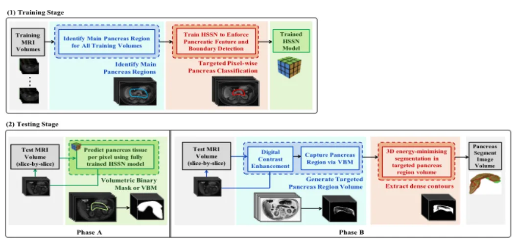
neighbouring tissue, and the boundary contrast can vary depending on the level of surrounding visceral fat. Differing from computer tomography (CT), the low resolution and slower imaging speed of MRI presents edge-based artefacts that blur the imaging boundaries between the pancreas and surrounding organs [3]. In existing research literature, pancreas segmentation tasks have been driven by two major methodologies: multi-atlas based [4, 5] coupled with statistical shape modeling [6], and in more recent years, convolutional neural networks (CNNs) or deep learning [7, 3, 8]. While CNNs have achieved higher quantitative accuracy scores in 2D medical image segmentation, such methods can exhibit discontinuity in predicting pancreatic regions between consecutive slices for an input volume. This paper presents a novel approach for automatic pancreas segmentation in MRI. As illustrated in Figure 1, the proposed method consists of two succes-sive stages. First, a CNN specialising in blurred boundary detection is trained to predict targeted pixel-wise pancreas tissue. This deep learning stage firstly identifies the main pancreas region (ROI) in a dataset of MRI volumes [8] by training a random forest on extracted texture and probability-wise features on image patches of 25×25 pixels. Next, inspired by the encoder-decoder archi-tecture of SegNet [9] a new model termed Hausdorff Sine SegNet (HSSN) is developed using the ROI data. A novel loss function incorporates the modified Hausdorff distance metric and a sinusoidal component to capture local boundary information, enforce edge detection and thus raise the true pancreas prediction rate on a 2D (slice-by-slice) basis. The testing stage consists of two phases. First, the output of the trained HSSN for a given test MRI volume encodes spatial in-formation to classify every pixel in each slice, thus forming a volumetric binary mask (VBM). The second phase generates dense contouring by further tackling the low dissimilarity between organ boundaries: a digital contrast enhancement model is utilised to improve the greyscale variation between surrounding back-ground classes within close proximity to the pancreas. A 3D energy-minimising algorithm performs refined segmentation on the enhanced pancreas that is fused with the VBM, producing greater consistency in spatial smoothness and predic-tion among successive slices.

The proposed method, which is evaluated on two MRI datasets with varying noise, outperforms the state-of-the-art approaches [8, 10–12], and moreover, sur-passes the performance of readily employed deep learning-based loss functions. Although this approach has been tested on pancreas segmentation, the method-ology is reproducible, scalable and generalisable to other organ segmentation tasks. The implementation is available athttps://github.com/med-seg/p.

2

Methodology

2.1 Training the HSSN

The proposed HSSN model has an encoder-decoder topology, as illustrated in Figure 2. The decoder network uses max-pooling indices to upsample low-resolution feature maps, consequently retaining high-frequency details to improve pancre-atic boundary delineation, and reducing the total number of trainable parameters in the decoders. Unlike other models that have been fine-tuned from pre-trained

Train HSSN to Enforce Pancreatic Feature and Boundary Detection

Identify Main Pancreas Regions

Targeted Pixel-wise Pancreas Classification

Identify Main Pancreas Region for All Training Volumes

Trained HSSN Model Volumetric Binary Mask or VBM Phase A

VBM Capture Pancreas Region via VBM Digital

Contrast Enhancement

Generate Targeted

Pancreas Region Volume Extract dense contours (1) Training Stage Pancreas Segment Image Volume 3D energy-minimising segmentation in targeted pancreas region volume Training MRI Volumes Test MRI Volume (slice-by-slice)

Predict pancreas tissue per pixel using fully trained HSSN model Test MRI Volume (slice-by-slice) Phase B (2) Testing Stage

Fig. 1: Overview of proposed approach. (1) develop the HSSN deep learning model using training MRI; and (2) apply the test MRI to generate segmented pancreas volume. CNNs using a large number of natural images [3, 13], this network is trained from scratch using exclusively pancreas datasets. Since this organ accounts for∼1% in a scan, there is a need to weight the loss differently based on the true class: Median frequency balancing [14] is utilised, in which the weight assigned to a class in the loss function is the ratio of the median of class frequencies computed on the entire training set divided by the class frequency. The HSSN also employs data augmentation of random reflections and translations to reduce overfitting [15], and further address problems caused by high shape variability.

Pooling indices

.

..

.

..

Pixel classification Boundary tracing of predicted pancreas region

Fig. 2: Overview of HSSN model. An encoder stage (5 blocks of HSSN-E) downsamples the MRI input through convolution, batch normalisation and ReLU. A decoder stage (5 blocks of HSSN-D) upsamples its input using the transferred pooling indices from its corresponding encoder to generate sparse feature maps. From here, convolution is performed with a trainable filter of weights to density the feature map. Resulting decoder output feature maps are fed to soft-max classifier for 2-channel pixel-wise classification of the input image as “pancreas” or “non-pancreas”.

Integrated Hausdorff-Sine Loss Function: A novel loss function is proposed for training the segmentation neural network. The optimisation of the modified Hausdorff distance and a sinusoidal functionality serves to reduce the bound-ary matching error and “enhance” a resulting pixel-wise pancreas prediction. Let TH andYH represent the ground-truth and network boundary predictions

4 H.Asaturyan et al.

respectively, where TH, YH ⊂ Rn such that |TH|,|YH| < ∞. Furthermore, tj

andyj∈ {0,1} are indexed pixel values inTH andYH respectively, and can be

viewed as boundary points. The Euclidean distance between a pointtj and set

of points,YHiss(tj, YH) = min yj∈YH

ktj−yjk, and the distance between a pointyj

and set of points, TH iss(yj, TH) = min tj∈TH kyj−tjk. IfεY = _|Y1 H| P yj∈YH s(tj, YH) andεT =_|T1 H| P tj∈TH

s(yj, TH), the modified Hausdorff distance loss,Lmhdis:

Lmhd= max{εY, εT} (1)

Thus, computing the gradient yields:

∂Lmhd ∂YH =      ∂ ∂YH (εY) ifεY > εT ∂ ∂YH (εT) ifεT < εY undefined ifεY =εT (2) An additional sinusoidal component increases non-linearity during network training and, empirically evaluated, raises the true positive predictions. IfT and

Y represent the ground-truth and network predictions, the lossLsine is defined:

Lsine=− 1 |Y| nC X i=1 sin(Ti) log2(Yi) (3)

wherenC= 2 is the number of classes (e.g.,Y1 refers to “pancreas” andY2

refers to “non-pancreas”). From here, computing the gradient yields:

∂Lsine ∂Yi =− 1 |Y| sin(Ti) Yilog10(2) (4) The model is updated via the combined gradients ofLsine andLmhd.

2.2 Testing Stage

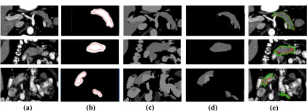
(A) Targeted Pancreas Binary Mask: The trained HSSN model performs pixel-wise prediction on each slice in a test MRI volume to generate a resulting volumetric binary mask (VBM). Columns (a) and (b) in Figure 3 displays three sample input slices in three different image volumes, and the corresponding pos-itive pancreas region (white mask) as predicted by the HSSN model. The red contouring in each image in column (b) is the ground-truth.

(a) (b) (c) (d) (e)

(B) Achieve Dense Contouring: The test MRI volume undergoes non-local means for denoising, after which a learned intensity model incorporates a sig-moid function to exhaustively differentiate pancreatic tissue against background classes. Every si-th slice transforms to C(si) = 1/(1 + exp [g(c−si)]), where g

controls the actual contrast, and c is the cut-off value representing the (nor-malised) greyscale value about whichg is changed [12, 16]. The VBM is applied to the enhanced image volume and processed through a 3D unsupervised energy-minimisation method via continuous max-flow [17], revealing detailed contouring as highlighted in Figure 3, column (c). The accurate HSSN predictions reduce the level of non-pancreatic tissue carried into the max-flow segmentation stage, as shown in Figure 3, column (d), eliminating the need for post-processing.

3

Experimental Results and Analysis

3.1 Datasets and Evaluation

Two expert-led annotated pancreas datasets are utilised. MRI-A and MRI-B contain 180 and 120 abdominal MRI scans (T2-weighted, fat suppressed), which have been obtained using a Philips Intera 1.5T and a Siemens Trio 3T scan-ner, respectively. Every MRI-A scan has 50 slices, each of size 384×384 with spacing 2mm, and 0.9766mm pixel interval in the axial and sagittal direction. Every MRI-B scan has 80 slices, each of size 320×260 with 1.6mm spacing, and 1.1875mm pixel interval in the axial and sagittal direction. The proposed approach is evaluated using the Dice Similarity Coefficient (DSC), precision (PC), recall (RC) and the Hausdorff distance (HSD) representing the maximum boundary deviation between the segmentation and ground-truth.

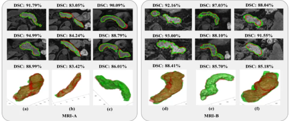
DSC: 83.42% DSC: 84.24% DSC: 83.05% DSC: 86.01% DSC: 88.79% DSC: 90.09% DSC: 88.99% DSC: 94.99% DSC: 91.79% (a) (b) (c) MRI-A DSC: 92.16% DSC: 93.00% DSC: 88.41% DSC: 85.70% DSC: 88.10% DSC: 87.03% DSC: 85.18% DSC: 88.04% DSC: 91.55% (d) (e) (f) MRI-B

Fig. 4: Segmentation results in six different MRI scans (volumes). Every column corre-sponds to a single MRI volume. From left, first row displays sample MRI axial slices with segmentation outcome (green) against ground-truth (red), and computed DSC. Second row displays 3D reconstruction of entire pancreas with computed DSC.

3.2 Network Implementation

The training and testing data are randomly split into 160 and 20 (MRI-A) and 100 and 20 (MRI-B). The HSSN model employs stochastic gradient descent

6 H.Asaturyan et al.

with parameters momentum (0.9), initial learning rate (0.001), maximum epochs (300) and mini-batch size (10). The mean time for model training is∼11 hours and the testing phase is∼7.5 minutes per MRI volume using an i7-59-30k-CPU at 3.50 Ghz. Future work can potentially reduce these run-times by a factor of 10 via multiple GeForce Titan X GPUs.

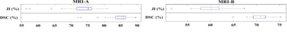
Fig. 5: Box plots of DSC and JI.

3.3 Analysis of Proposed Approach

Figure 4 displays the final segmentation results in six MRI scans, equally split between MRI-A and MRI-B. Columns (a, b, c) are part of MRI-A, yet there is high variation between intensity and contrast in the original axial MRI slices. Columns (d, e, f) corresponds to exemplars from MRI-B. As reflected in Figure 5, 85% of MRI-A compared to 95% in MRI-B segmentations score above 80% in DSC, demonstrating the robust performance of the approach with respect to poor image quality, intensity distribution and spatial dimensions.

0.05 0.15 0.25 0.35 0.45 0.55 0.65 0.75 0.85 0.95 Probability Threshold 45 50 55 60 65 70 75 80 85 DSC(%)

MRI-A and MRI-B

Hausdorff-Sine Hausdorff Cross-Entropy Dice Jaccard

Fig. 6: DSC across threshold ranges [0.05, 0.95] via multiple loss functions:

0 0.1 0.2 0.3 0.4 0.5 0.6 0.7 0.8 0.9 1

False positive rate

0 0.1 0.2 0.3 0.4 0.5 0.6 0.7 0.8 0.9 1

True positive rate

ROC for MRI-A and MRI-B

Hausdorff-Sine Hausdorff Cross-Entropy Dice Jaccard

Fig. 7: Averaged ROC curves via mul-tiple loss functions.

Hausdorff-Sine Loss: Figure 6 compares the segmentation results (in DSC) using Hausdorff-Sine and the loss functions, Hausdorff, Cross-entropy, Dice [18] and Jaccard [19] in the probability range [0.05,0.95]. The cross-entropy penalises true positive predictions, forcing the “optimum” probability to approximately 0.5. Although the Dice loss minimises the class distribution distance, squar-ing the weights in the backpropagation stage causes instability and a higher rate of false negative predictions. Similarly, the Jaccard loss suffers from low true positive predictions. Empirically tested, the Hausdorff loss minimises the maximum deviation between a prediction and desired outcome; however, the addition of a sinusoidal component increases non-linearity during training, and thus Hausdorff-Sine achieves improved true positive predictions across differing thresholds while delivering strong discrimination of true negatives. The ROC curves in Figure 7 highlight the inferior performance of other loss functions in

the extremely unbalanced segmentation, whereas Hausdorff-Sine generally im-proves the true positive accuracy results.

Phase B of Testing Stage Integrating the second phase (B) produces contex-tual boundary information that is essential for accurate segmentation in biomed-ical imaging. Figure 3, column (b) and column (e) visibly highlights the differ-ences in segmentation boundary delineation against the ground-truth before and after this phase. Thus, the mean HSD metric confirms less deviation from the ground-truth (see Table 1 and 2) by approximately 1 mm, and furthermore, the mean DSC raises by approximately 4% in both MRI-A and MRI-B.

Table 1: Deep learning model performance using state-of-the-art loss functions versus the integrated novel Hausdorff and Hausdorff-Sine loss. Datasets MRI-A and MRI-B are evaluated in 9-fold and 6-fold cross-validation (FCV), respectively. DSC, PC, RC and HSD are presented as mean±standard deviation.

MRI-A: Train/Test (160/20) 9-FCV Loss DSC(%) PC(%) RC(%) HSD(mm) CE 77.9±3.6 88.4±6.18 95.6±2.26 12.4±5.5 Dice 63.5±9.1 63.8±20.0 86.8±10.5 16.8±5.3 Jac 63.2±9.6 62.5±19.8 87.1±10.0 17.0±5.4 Haus 78.4±6.1 89.5±9.11 96.2±4.06 12.7±4.9 Haus-Sin 79.7±4.0 93.2±7.46 97.2±2.67 11.2±3.6 MRI-B: Train/Test (100/20) 6-FCV Loss DSC(%) PC(%) RC(%) HSD(mm) CE 79.9±4.33 92.6±6.89 96.3±2.76 10.5±3.34 Dice 67.1±12.8 77.2±15.1 85.2±16.8 21.4±12.3 Jac 68.6±6.96 68.3±16.9 88.5±8.34 17.9±7.58 Haus 81.0±4.25 94.8±3.84 98.3±2.28 10.2±4.17 Haus-Sin 82.1±2.99 97.7±2.50 99.1±0.78 10.0±6.63

Table 2: DSC, PC, RC and HSD as mean ±standard deviation [lowest, highest] for automatic segmentation methods. Datasets MRI-A and MRI-B are evaluated in 9-fold and 6-fold cross-validation (FCV), respectively.

MRI-A: Train/Test (160/20) 9-FCV Method DSC(%) PC(%) RC(%) HSD (mm) U-Net [10] 66.8±8.8 [42.3, 77.3] 71.3±4.4 [62.9, 80.5] 85.1±4.8 [76.9, 88.16] 16.9±5.8 [8.22, 24.1] Cascaded-CNN [8] 52.7±6.9 [34.4, 60.7] 64.0±4.1 [50.4, 68.0] 75.2±4.6 [68.1, 78.25] 21.5±9.3 [15.7, 38.6] Dense V-Net [11] 73.6±6.1 [49.6, 78.8] 86.1±3.3 [78.5, 88.5] 94.6±3.4 [82.8, 96.37] 14.4±7.2 [6.63, 20.5] Geo-Desc [12] 78.2±5.8 [67.1, 86.3] 85.3±9.7 [70.8, 98.9] 93.9±9.5 [52.5, 99.13] 13.8±4.4 [6.11, 18.4] Proposed 84.1±4.6 [72.1, 89.6] 95.5±6.3 [71.7, 99.7] 97.6±3.0 [89.9, 100.0] 10.6±3.7 [6.184, 18.4] MRI-B: Train/Test (100/20) 6-FCV Method DSC(%) PC(%) RC(%) HSD (mm) U-Net [10] 72.8±6.0 [58.9, 80.8] 83.8±3.1 [74.2, 87.46] 94.6±3.5 [82.8, 95.72] 14.0±8.1 [6.82, 21.7] Cascaded-CNN [8] 54.8±5.1 [44.4, 65.7] 64.3±3.5 [59.5, 67.91] 76.2±3.7 [69.9, 79.64] 22.3±8.6 [16.0, 37.5] Dense V-Net [11] 74.0±5.3 [65.1, 80.3] 85.4±3.1 [78.5, 89.74] 93.0±3.8 [84.9, 96.35] 16.7±7.0 [8.46, 19.8] Geo-Desc [12] 81.2±5.0 [72.6, 85.8] 84.7±5.8 [73.1, 93.64] 84.6±8.2 [69.2, 97.28] 14.7±4.1 [8.13, 17.6] Proposed 85.7±2.3 [79.9, 90.3] 96.1±3.6 [86.7, 100.0] 99.3±0.7 [99.9, 100.0] 9.08±2.0 [4.87, 14.8]

Comparison with the State-of-the-art: Table 2 highlights the proposed approach outperforming state-of-the-art methods [8, 10–12] in terms of accuracy and statistical stability despite employing non-organ optimised protocol data.

4

Conclusion

This paper presents a novel approach for automatic pancreas segmentation in MRI volumes generated from different scanner protocols. Combined with the proposed Hausdorff-Sine loss, an encoder-decoder network reinforces pancreatic boundary detection in MRI slices, outperforming the rate of true positive pre-dictions compared to multiple loss functions. In the later stage, a 3D hybrid energy-minimisation algorithm addresses the intensity consistency problem that is often the case when segmenting image volumes on a 2D basis. The proposed approach generates quantitative accuracy results that surpass reported state-of-the-art methods, and moreover, preserve detailed contouring.

8 H.Asaturyan et al.

References

1. Mavin Macauley, Katie Percival, Peter E. Thelwall, Kieren G. Hollingsworth, and Roy Taylor. Altered Volume, Morphology and Composition of the Pancreas in Type 2 Diabetes. PLOS ONE, 10(5):1–14, 2015.

2. Ahmad Omeri, Shunro Matsumoto, Maki Kiyonaga, Ryo Takaji, Yasunari Yamada, Kazuhisa Kosen, Hiromu Mori, and Hidetoshi Miyake. Contour variations of the body and tail of the pancreas: evaluation with mdct. J Radiol, 35(6):310–318, 2017.

3. Jinzheng Cai, Le Lu, Zizhao Zhang, Fuyong Xing, Lin Yang, and Qian Yin. Pan-creas Segmentation in MRI Using Graph-Based Decision Fusion on Convolutional Neural Networks, pages 442–450. Springer International Publishing, 2016. 4. Toshiyuki Okada, Marius George Linguraru, Yasuhide Yoshida, Masatoshi Hori,

Ronald M. Summers, Yen-Wei Chen, Noriyuki Tomiyama, and Yoshinobu Sato. Abdominal multi-organ segmentation of ct images based on hierarchical spatial modeling of organ interrelations. InAbdom Radiol, pages 173–180. Springer Berlin Heidelberg, 2012.

5. Akinobu Shimizu, Tatsuya Kimoto, Hidefumi Kobatake, Shigeru Nawano, and Kenji Shinozaki. Automated pancreas segmentation from three-dimensional contrast-enhanced computed tomography. Int J Comput Assist Radiol Surg, 5(1):85–98, 2010.

6. Toshiyuki Okada, Marius George Linguraru, Masatoshi Hori, Ronald Summers, Noriyuki Tomiyama, and Yoshinobu Sato. Abdominal multi-organ segmentation from CT images using conditional shape–location and unsupervised intensity pri-ors. Med Image Anal, 26:1–18, 2015.

7. Jinzheng Cai, Le Lu, Yuanpu Xie, Fuyong Xing, and Lin Yang. Improving deep pancreas segmentation in CT and MRI images via recurrent neural contextual learning and direct loss function. CoRR, abs/1707.04912, 2017.

8. Amal Farag, Le Lu, Holger R Roth, Jiamin Liu, Evrim Turkbey, and Ronald M Summers. A bottom-up approach for pancreas segmentation using cascaded su-perpixels and (deep) image patch labeling. IEEE Trans. Image, 26(1):386–399, 2017.

9. Vijay Badrinarayanan, Alex Kendall, and Roberto Cipolla. Segnet: A deep convo-lutional encoder-decoder architecture for image segmentation. arXiv:1511.00561, 2015.

10. Olaf Ronneberger, Philipp Fischer, and Thomas Brox. U-Net: Convolutional Net-works for Biomedical Image Segmentation, pages 234–241. Springer International Publishing, Cham, 2015.

11. Eli Gibson, Francesco Giganti, Yipeng Hu, Ester Bonmati, Steve Bandula, Kurinchi Gurusamy, Brian Davidson, Stephen P Pereira, Matthew J Clarkson, and Dean C Barratt. Automatic multi-organ segmentation on abdominal CT with dense V-Networks. IEEE Trans Med Imaging, 2018.

12. Hykoush Asaturyan, Antonio Gligorievski, and Barbara Villarini. Morphological and multi-level geometrical descriptor analysis in ct and mri volumes for automatic pancreas segmentation. Comput Med Imaging Graph, 75:1–13, 2019.

13. Saining Xie and Zhuowen Tu. Holistically-nested edge detection. InProc IEEE ICCV, pages 1395–1403, 2015.

14. David Eigen and Rob Fergus. Predicting depth, surface normals and semantic labels with a common multi-scale convolutional architecture. In Proc IEEE Int Conf Comput Vis, pages 2650–2658, 2015.

15. Luis Perez and Jason Wang. The effectiveness of data augmentation in image classification using deep learning. arXiv:1712.04621, 2017.

16. Asaturyan Hykoush and Barbara Villarini. Hierarchical framework for automatic pancreas segmentation in MRI using continuous max-flow and min-cuts approach. InImage Analysis and Recognition, pages 562–570. Springer International Publish-ing, 2018.

17. Jing Yuan, Egil Bae, and Xue-Cheng Tai. A study on continuous max-flow and min-cut approaches. InProc IEEE Comput Soc Conf Comput Vis Pattern Recognit, pages 2217–2224, 2010.

18. F. Milletari, N. Navab, and S. A. Ahmadi. V-Net: Fully convolutional neural networks for volumetric medical image segmentation. InFourth Int. Conf. 3DV, pages 565–571, 2016.

19. Md Atiqur Rahman and Yang Wang. Optimizing intersection-over-union in deep neural networks for image segmentation. InISVC, pages 234–244. Springer, 2016.