NBER WORKING PAPER SERIES
GLOBAL FORCES AND MONETARY POLICY EFFECTIVENESS
Jean Boivin
Marc Giannoni
Working Paper 13736
http://www.nber.org/papers/w13736
NATIONAL BUREAU OF ECONOMIC RESEARCH
1050 Massachusetts Avenue
Cambridge, MA 02138
January 2008
Prepared for the NBER conference on International Dimensions of Monetary Policy in Girona (Spain),
June 2007. We thank conference participants, in particular Olivier Blanchard, Jordi Galí, Mark Gertler,
Larry Meyer, Benoît Mojon, Lucrezia Reichlin, Chris Sims, and Michael Woodford for very valuable
discussions and comments, and Guilherme Martins for excellent research assistance. We are also grateful
to the National Science Foundation for financial support (SES-0518770). The views expressed herein
are those of the author(s) and do not necessarily reflect the views of the National Bureau of Economic
Research.
NBER working papers are circulated for discussion and comment purposes. They have not been
peer-reviewed or been subject to the review by the NBER Board of Directors that accompanies official
NBER publications.
Global Forces and Monetary Policy Effectiveness
Jean Boivin and Marc Giannoni
NBER Working Paper No. 13736
January 200
8
JEL No. C32,C53,E31,E32,E40,F41
ABSTRACT
In this paper, we quantify the changes in the relationship between international forces and many key
US macroeconomic variables over the 1984-2005 period, and analyze changes in the monetary policy
transmission mechanism. We do so by estimating a Factor-Augmented VAR on a large set of US and
international data series. We find that the role of international factors in explaining US variables has
been changing over the 1984-2005 period. However, while some US series have become more correlated
with global factors, there is little evidence suggesting that these factors have become systematically
more important. We don't find strong evidence of a change in the transmission mechanism of monetary
policy due to global forces. Taking our point estimates literally, global forces do not seem to have
played an important role in the US monetary transmission mechanism between 1984 and 1999. In
addition, since the year 2000, the initial response of the US economy following a monetary policy
shock --- the first 6 to 8 quarters --- is essentially the same as the one that has been observed in the
1984-1999 period. However, point estimates suggest that the growing importance of global forces
might have contributed to reducing some of the persistence in the responses, two or more years after
the shocks. Overall, we conclude that if global forces have had an effect on the monetary transmission
mechanism, this is a recent phenomenon.
Jean Boivin
HEC Montréal
3000, chemin de la Côte-Sainte-Catherine
Montréal (Québec)
Canada H3T 2A7
and NBER
Marc Giannoni
Columbia Business School
3022 Broadway, Uris Hall 824
New York, NY 10027-6902
and NBER
1
Introduction
In many respects, the economic integration of the U.S. economy with the rest of the world has deepened in the last two decades. International trade has continued to expand more rapidly than economic activity in industrialized countries. For the US, the amount of goods and services imported and exported which represented 18% of GDP in the mid-1980’s represents more than 27% in 2005. But the globalization of finance has shown a much more dramatic development. During the same period, the ratio of foreign assets and liabilities to GDP has increased from approximately 80% to more than 300% in the 23 most industrialized economies, according to Lane and Milesi-Ferretti (2006). As global economic integration is spreading, it is often argued that macroeconomic variables in one country – whether they pertain to measures of economic activity, inflation, or interest rates – should increasingly reflect events occurring in the rest of the world.1
Such developments raise naturally two sets of questions which we attempt to address in this paper. First, to what extent have international factors affected the determination of key macroeco-nomic variables in the US economy? Is it the case that with the recent globalization, this economy has become more strongly affected by international factors? Second, has the very rapid globaliza-tion of finance weakened the ability of US monetary policy to influence domestic financial market conditions, and through it, the rest of the economy? In other words, does a change in the Federal Funds rate have a smaller impact on the US economy now than it used to?
Central bankers and economists in the financial press have pointed out the fact that while the US central bank raised the Federal funds rate target by 425 basis points between June 2004 and July 2006, long-term rates remained at historically low levels with the ten-year Treasury bond yield increasing by less than 40 basis points and the twenty-year yield actually falling by 20 basis points during that time. This phenomenon, which former Federal Reserve Chairman Alan Greenspan labeled “conundrum” highlights the fact that US long-term interest rates may have become more dependent on international factors than had been observed historically. As then Governor Bernanke 1For example, the President of the Federal Reserve Bank of Dallas, Richard Fisher, and Michael Cox (2007) have
argued that domestic inflation may be increasingly determined in the rest of the world. Advocating a “new inflation equation,” they conclude that “globalization has been changing how we consume as well as the way we do business. It’s high time economic doctrine caught up.” The Economist (2005), citing Stephen Roach, chief economist of Morgan Stanley, and the 2005 annual report of the Bank for International Settlements suggests that global forces have become more important relative to domestic factors in determining inflation in individual countries.
(2005) explained, a more extensive globalfinancial integration and the increased amount of savings outside the US – in particular in developing economies – may have resulted in a “global saving glut” which may have put downward pressures on long-term interest rates. A casual look at such recent historical episodes raises the possibility that the long-term yields may respond less to changes in Federal funds rates than in the past. Given that monetary policy does at least in part affect the economy through its effect on long-term rates, it is natural to wonder about the implications of the globalization of finance for the effectiveness of monetary policy. Certainly, the answers to such questions have key implications for a proper understanding of the determinants of economic fluctuations, and for policy.
To address these questions, we provide in this paper an empirical assessment of the synchro-nization between international factors and key US economic variables. We then investigate whether the importance of these global forces has changed for the US economy over the last two decades, and how such a possible change has affected the transmission of monetary policy.
The general empirical framework that we consider is a factor-augmented vector autoregression model (FAVAR), as described in Bernanke, Boivin and Eliasz (2005), but extended to explicitly include international or “global” factors. One of its key features is to provide estimates of macro-economic factors that affect the data of interest by systematically exploiting all information from a large set of economic indicators. In our application, we estimate the empirical model based on the information from a large number of macroeconomic indicators, and disaggregated data for the US, as well as a large set of macroeconomic indicators for the 15 major US trade partners. By identifying US monetary policy shocks, this framework allows us to uncover the transmission of such shocks to a large set of macroeconomic indicators. Our interest in studying the responses to monetary policy shocks does not reside in the fact that these shocks are important. In fact, it is well-known that they contribute only little to US output fluctuations. Rather, we find the responses to such shocks interesting as they allow us to trace out the effects of monetary policy on the economy.
Many studies have provided evidence that key macroeconomic variables display substantial comovements across countries. For instance, Kose, Otrok and Whiteman (2003), analyzing output, consumption and investment data from 60 countries over the 1960-1990 period, document that a
large fraction of business cycles fluctuations of developed economies is accounted by a common world factor. The latter factor – a component of economic activity which is common to all countries considered – explains more than one third of output fluctuations in the US and in Europe.2 Ciccarelli and Mojon (2005) argue that inflation in industrialized economies is also largely a global phenomenon: they find that on average, about 70% of inflation variance is attributable to a common global factor given by the component of inflation that is common across countries. Moreover, Ehrmann, Fratzscher, and Rigobon (2005) show that shocks to money, bond and equity markets result in substantial spillovers between the US and Europe.
Other researchers have recently examined whether the importance of such comovements across regions has changed over time. The evidence regarding the output synchronization is mixed. Kose, Prasad and Terrones (2003) report evidence of stronger comovements of output in industrialized countries with a world factor, since the early 1980’s, than in the preceding two decades. However, Doyle and Faust (2005), testing for changes in comovements among real activity measures for the G7 countries find very few statistically significant changes over the 1960-2000 period. When looking at their point estimates, they even find some evidence of a fall in the correlation across countries since the early 1980s. Such a reduced synchronization is in fact consistent withfindings of Helbling and Bayoumi (2003), Monfort, Renne, Ruffer and Vitale (2003), Heathcote and Perri (2004), Stock and Watson (2005), and Kose, Otrok and Whiteman (2005). According to Stock and Watson (2005), and Kose et al. (2005), the fact that the output correlations across countries were particularly high in the 1970s may reflect unusually strong common shocks, such as large movements in oil prices, during that period. These authors thus argue that the reduction in the 2Similar comovements in economic activity have been documented for more restricted sets of countries. Gerlach
(1988) found that industrial production is positively correlated across several OECD countries. Backus, Kehoe and Kydland (1995) and Baxter (1995) found that business cycles share similarities in major industrial economies. Gregory, Head and Raynauld (1997) in an early estimation of a factor model on economic activity data for the G7 countries, detected a significant common factor across countries. Bergman, Bordo and Jonung (1998), analyzing more than one hundred years of data, found that the synchronization in activity across 13 industrialized countries remains strong regardless of the monetary regime. Forni, Hallin, Lippi and Reichlin (2000), proposing a generalized dynamic factor model and applying it to data of 10 European economies,find that a common European activity factor explains between 35% and 96% of the volatility in countries’ GDP. Clark and Shin (2000), similarlyfind that a common factor accounts substantial variations in industrial production of European economies, and Lumsdaine and Prasad (2003), examining correlations between industrial output in 17 OECD countries and a common component,find evidence of a world business cycle and of a European business cycle. Canova, Ciccarelli and Ortega (2004), estimating a Bayesian panel VAR model on G7 datafind also a significant world business cycle, butfind no evidence of a cycle specific to the Euro area, in contrast to some of the other studies.
volatility of common international shocks since in the early 1980s, compared to the 1960s and 1970s, provides an important explanation for the reduced synchronization among G7 countries since the early 1980s, and that the correlation in output across countries would have been larger, had the international common shocks been as important in the 1980s and the 1990s, as they were in the 1960s and 1970s.
In addition, some authors have argued that the development of trade in goods and services, especially with low-cost producing economies such as China and India may have altered the rela-tionship between some measure of the output gap and domestic inflation (see, e.g., Rogoff(2004), Borio and Filardo (2006), Ihrig et al. (2007)).
While we also seek to characterize changes US macroeconomic dynamics due to global forces, our paper distinguishes itself from the papers just mentioned in several respects.
First, in general, global co-movements among macro variables could arise from the presence of exogenous global – or worldwide – shocks, or from the international transmission of domestic shocks. Our central focus in this paper is the implications for monetary policy of the changes in the role of global forces. It is thus important to stress that while we allow for the presence of global shocks like in many of the papers just cited, our interest will be mainly on the characterization of the international transmission of regional shocks. In particular, we determine to what extent the transmission of U.S. monetary policy shocks – as measured by exogenous changes in the Federal funds rate – to key US economic variables such as long-term interest rates, output, inflation, and so on, has been altered by global forces.
Second, in order to identify the monetary transmission mechanism, we jointly model multiple dimensions of the US economy. Thus, rather than restricting ourself to the comparison of a single type of measures across regions of the world – e.g. only economic activity measures or only inflation measures – we adopt a more general and encompassing approach which allows us to compare a set of factors summarizing the US macroeconomic dynamics with those summarizing the rest of the world’s macroeconomic dynamics. Another contribution is hence to consider a much broader set of macroeconomic indicators than has been used before in order to document the changes in the importance of global forces for the determination of US measures of real activity, inflation, interest rates and various other series.
Finally, we focus on the evolution since 1984. Our sample includes the period during which the globalization offinancialflows accelerated significantly and allows us to sidestep an important issue: the considerable changes that occurred in the preceding decade. The period of large common shocks, in the 1970s and the early 1980s, during which the business cycles of many countries were strongly correlated, was followed in the US by a rapid adjustment – called “great moderation” – to a regime characterized by lower output volatility.3 Some studies have explained the reduction in volatility with a reduced volatility of shocks (e.g., Stock and Watson (2002a), Sims and Zha (2006), Justiniano and Primiceri (2006), Smets and Wouters (2007)). In addition, as documented in Clarida, Galí and Gertler (2000), Boivin (2006), Cogley and Sargent (2001, 2005), Boivin and Giannoni (2002, 2006a), the systematic response of US monetary policy tofluctuations in inflation and output has changed significantly around 1980, revealing a greater tendency to stabilize inflation fluctuations. As Boivin and Giannoni (2006a) emphasize, such a change in policy can explain in large part why the responses of output and inflation to an unexpected change in the Federal funds rate of a given size have been much smaller since the early 1980s, than they were in the 1960s and 1970s. By considering the period after 1984, i.e., a period during which both the variance of the shocks may reasonably be assumed to have remained constant and the systematic monetary policy rule has not been found to have dramatically changed, we hope to better isolate the effect of international factors.
It is important to stress, however, that our sample is relatively short: it contains a bit more than 20 years of quarterly data. We expect a priori that this will make statistical relationships harder to detect and will constitute an important constraint on the richness of the models that we can contemplate in the empirical exercise below. This is an important sense in which we see our analysis as an exploration of how important global forces might have become for the US economy. But as the results seem to suggest, there is still sufficient statistical information in the sample that allows us to learn something useful about changes in the economy in the recent past.
Our findings can be summarized as follows. First, we find that common factors capture on 3
Many researchers have documented a sharp drop in the volatility of the US real GDP in the early 1980s (see, e.g., McConnell and Perez-Quiros (2000), Blanchard and Simon (2001), Boivin and Giannoni (2002), Stock and Watson (2002a)). Stock and Watson (2005) show that other G7 countries with the exception of France have similarly experienced lower output volatility since the mid-1980s compared to the previous decades.
average a sizable fraction of thefluctuations in US macroeconomic indicators. This provides support for the use of our empirical model. Second, there is evidence that the role of international factors in explaining US variables has been changing over the 1984-2005 period, but this evolution is not systematic across series, and it is difficult to see a pattern suggesting that they have become generally more important. Some variables such as the long-term interest rates, as well as import and export prices, however, do display a systematic increase of their correlation with global factors throughout our sample.
We don’t find strong statistical evidence of a significant change in the transmission mechanism of monetary policy due to global forces. Taking our point estimates literally, global forces do not seem to have played an important role in the US monetary transmission mechanism between 1984 and 1999. Also, since 2000, the initial response of the US economy following a monetary policy shock – the first 6 to 8 quarters – is essentially that same as the one that has been observed in the 1984-1999 period. However, point estimates suggest that the growing importance of global forces might have contributed to reducing some of the persistence in the responses, two or more years after the shocks.
Overall, we conclude that if global forces have had an effect on the monetary transmission mechanism, this is a recent phenomenon. This means however that we will need more data before we can get strong statistical conclusions on this question.
The rest of the paper is organized as follows. In Section 2, we describe the econometric frame-work adopted and the estimation approach. In Section 3, we present empirical results on the comovements between international factors and US data, and document changes in these relation-ships over the last two decades. In Section 4, we document to what extent the role of global factors has changed the transmission mechanism of monetary policy. Section 5 concludes.
2
Econometric Framework: FAVAR
One key objective of this study is to evaluate the importance of the rest of the world in the transmission of US monetary policy. That is, we seek to estimate to what extent the response of the rest of the world’s economy enhances or mitigates the effect of US monetary policy on the US
economy, and, importantly, whether this has changed over time. The FAVAR model described in Bernanke, Boivin and Eliasz (2005) (BBE) provides a natural framework to address these questions. In this section, we describe the empirical model and our estimation approach.
2.1
Description of FAVAR
The econometric framework that we consider is based on the FAVAR extended to include interna-tional factors. We consider two regions: the US economy and the rest of the world, which we denote with *. We assume that in each region, the state of the economy, which is possibly unobserved, can be summarized by aK×1vectorCtin the US, and aK∗×1vectorCt∗for the rest of the world. We
measure the state of the economy in each region with large vectors of macroeconomic indicators, denoted byXtfor the US, andXt∗ for the rest of the world. These vectors are of dimension N×1
and N∗×1respectively. The indicators are assumed to relate to the state of the economy in each
region according to the observation equations
Xt = ΛCt+et (1)
Xt∗ = Λ∗Ct∗+e∗t (2)
whereΛandΛ∗are matrices of factor loadings of appropriate dimensions, and theN×1(respectively N∗×1)vectorsetande∗
t contain (mean-zero) series-specific components that are uncorrelated with
the common componentsCt(respectivelyCt∗), but are allowed to be serially correlated and weakly
correlated across indicators. The number of common factors is assumed to be small relative to the number of indicators, i.e.,N > K andN∗ > K∗.
Under this structure,CtandCt∗constitute two sets of components which are common to all data
series in the respective region and in general correlated across regions. Equations (1)—(2) reflect the fact that the common factors represent pervasive forces that drive the common dynamics of the data, and summarize at each date the state of the economy in each region. The variables inXt
are thus noisy measures of the underlying unobserved factors Ct. Note that it is in principle not
capture arbitrary lags of some fundamental factors.4 The unobserved factors should reflect general region-specific economic conditions such as “economic activity,” the “general level of prices,” the level of “productivity,” and key dimensions of the interest-rate term structure, which may not easily be captured by a few time series, but rather by a wide range of economic variables.
The dynamics of the common factors are modeled as a structural VAR
Φ0 ⎡ ⎢ ⎣ C ∗ t Ct ⎤ ⎥ ⎦=Φ(L) ⎡ ⎢ ⎣ C ∗ t−1 Ct−1 ⎤ ⎥ ⎦+ ⎡ ⎢ ⎣ v ∗ t vt ⎤ ⎥ ⎦ (3)
where Φ0 is a matrix of appropriate size on which we will later impose some restrictions,Φ(L) is a conformable lag polynomial of finite order, and the “structural” shocks vt and vt∗ are assumed
to be iid with mean zero and diagonal covariance matrix Q and Q∗ respectively. While these shocks are uncorrelated, anyone of these shocks may affect common factors of the other region immediately or over time, through the off-diagonal elements ofΦ0 and Φ(L).This structural VAR has a reduced-form representation obtained by premultiplying on both sides of (3) by Φ−01 :
⎡ ⎢ ⎣ C ∗ t Ct ⎤ ⎥ ⎦= ⎡ ⎢ ⎣ Ψ11(L) Ψ12(L) Ψ21(L) Ψ22(L) ⎤ ⎥ ⎦ ⎡ ⎢ ⎣ C ∗ t−1 Ct−1 ⎤ ⎥ ⎦+ ⎡ ⎢ ⎣ u ∗ t ut ⎤ ⎥ ⎦ (4)
where the reduced-form innovations ut andu∗t are cross-correlated.
Since we will ultimately be interested in characterizing the effects of monetary policy on the economy, we include in the vector of US common components an observable measure of the mon-etary policy stance. As in most related VAR applications, we assume that the Federal funds rate, Rt, is the policy instrument. The latter will be allowed to have pervasive effect throughout the
economy and will thus be considered as a common component of all US data series. We thus write
Ct= ⎡ ⎢ ⎣ Ft Rt ⎤ ⎥ ⎦,
whereFtis a vector of latent macroeconomic factors summarizing the behavior of the US economy.
2.2
Interpreting the FAVAR structure in an international context
The empirical model we just laid out is a dynamic factor model that links a large set of observable indicators to a small set of common components through the observation equations (1)—(2). The evolution of these common components is specified by the transition equation (3) or its reduced-form representation (4). It is useful to spell out more clearly the economic interpretation of this empirical model and, in particular, the relationship with possible underlying structural models.
As in Bernanke, Boivin and Eliasz (2005) and in Boivin and Giannoni (2006b), we interpret the unobserved factors,CtandCt∗ as corresponding to theoretical concepts or variables that would
enter a structural macroeconomic model. For instance, open-economy dynamic general equilibrium models such as those of Benigno and Benigno (2001), Clarida, Galí, and Gertler (2002), Lubik and Schorfheide (2005), and those of many papers collected in Galí and Gertler (2007) fully characterize the equilibrium evolution of inflation, output, interest rates, net exports and other variables in two regions. In terms of the notation in our empirical framework, all of these variables would be inCt
and Ct∗. The dynamic evolution of these variables implied by such open-economy models can be
approximated by an unrestricted VAR of the form (4).5 If all of these macroeconomic concepts were perfectly observed, the system (4) would boil down to a standard multi-country VAR and could be estimated directly, as in, e.g., Eichenbaum and Evans (1995), Grilli and Roubini (1995,1996), Cushman and Zha (1997), Kim and Roubini (2000), Scholl and Uhlig (2006). In such a case, there would be no need to use the large set of indicatorsXt.
However, there are reasons to believe that not all relevant concepts are perfectly observed. First, some macroeconomic concepts are simply measured with error.6 Second, some of the
macroeco-nomic variables which are key for the model’s dynamics may be fundamentally latent. For instance, the concept of “potential output” often critical in monetary model cannot be measured directly. By using a large data set, one is able to extract empirically the components that are most important in explaining fluctuations in the entire data set. While each common component does not need to represent any single economic concept, the common components Ct and Ct∗ should constitute a
5For a formal description of the link between the solution of a DSGE model in state-space form and a VAR see,
e.g., Fernández-Villaverde, Rubio-Ramírez, Sargent and Watson (2007) and references therein.
6Boivin and Giannoni (2006b) argue, for example, that inflation is imperfectly measured by any single indicator,
linear combination of all of the relevant latent variables driving the set of noisy indicatorsXt and
Xt∗,to the extent that we extract the correct number of common components from the data set.
An advantage of this empirical framework is that it provides, both for the US and the inter-national data sets, summary measures of the state of these economies at each date, in the form of factors which may summarize many features of the economy. We thus do not restrict ourselves simply to measures of inflation or output. Another advantage of our approach, as BBE argue, is that this framework should lead to a better identification of the monetary policy shock than standard VARs, because it explicitly recognizes the large information set that the Federal Reserve and financial market participants exploit in practice, and also because, as just argued, it does not require to take a stand on the appropriate measures of prices and real activity which can simply be treated as latent common components. Moreover, for a set of identifying assumptions, a natural by-product of the estimation is to provide impulse response functions for any variable included in the data set. This is particularly useful in our case, since we want to understand the effect of globalization on the transmission of monetary policy to a wide range of economic variables.
The empirical model (1)—(2) and (4) provides a convenient decomposition of all data series into components driven by the US factorsCt(i.e., the Federal funds rate and other US latent factorsFt),
non-US latent factors Ct∗, and by series-specific components unrelated to the general state of the economies,et ore∗t.For instance, (1) specifies that indicators of measures of US economic activity
or inflation are driven by the Federal funds rate Rt, US latent factors Ft,and a component that
is specific to each individual series (representing e.g., measurement error or other idiosyncrasies of each series). The dynamics of the US common components are in turn specified by (4).
Note that the factorsCtandCt∗summarizing macroeconomic conditions in the US, respectively
in the rest of the world, may be affected both by their own region-specific shocks and by worldwide or “global” shocks. In fact, since reduced-form innovationsutandu∗t may be cross-correlated, they
could be expressed as the sum of a component that is common both the US and the rest of the world, possibly due to “global” shocks and a component that is exclusively region specific. The
reduced-from VAR may thus be rewritten as
Ct∗ = Ψ11(L)Ct∗−1+Ψ12(L)Ct−1+Γ1gt+ε∗t (5)
Ct = Ψ21(L)Ct∗−1+Ψ22(L)Ct−1+Γ2gt+εt (6)
where gt is a vector of “global” exogenous shocks, and ε∗t, εt are disturbances that are specific to
each region and uncorrelated across regions.7
2.3
Estimation
As in Stock and Watson (2002b) and BBE, we estimate our empirical model using a variant of a two-step principal component approach which we briefly outline here. We refer to these papers for a more detailed description.
Thefirst step consists of extracting principal components from XtandXt∗ to obtain consistent
estimates of the common factors under the structure laid out. In the second step, the Federal funds rate is added to the estimated factors and the VAR in equation (4) is estimated. Note that in the first step, BBE do not impose the constraint that the Federal funds rate is one of the common components. So if this interest rate is really a common component, it should be captured by the principal components. To remove the Federal funds rate from the space covered by the principal components, BBE perform a transformation of the principal components exploiting the different behavior of what they call “slow moving” and “fast moving” variables, in the second step. Our implementation is slightly different, however. We adopt a more direct approach which consists of imposing the constraint that Federal funds rate is one of the factors in the first-step estimation. This guarantees that the estimated latent factors recover dimensions of the common dynamics not captured by the Federal funds rate.8 To do so, we adopt the following procedure in the first step of the estimation. Starting from an initial estimate ofFt, denoted byFt(0) and obtained as thefirst
K−1 principal components of Xt,we iterate through the following steps:
7In this respect,Ct andC∗
t have a different interpretation than the world factors estimated by, e.g., Gregory et al. (1997), Forni et al. (2000), Kose et al., (2003), Ciccarelli and Mojon (2005). While these authors estimate a world factor and orthogonal region (or country)-specific factors, our estimatedCt andC∗
t contain bothfluctuations in regional and world factors.
1. RegressXt on Ft(0) and Rt, to obtain λˆ (0) R 2. Compute X˜t(0)=Xt−λˆ (0) R Rt
3. EstimateFt(1) as thefirst K−1principal components of X˜t(0)
4. Back to 1.
Having estimated the factorsCtandCt∗ and the factor loadingsΛ,Λ∗,we can estimate the VAR
(4). As we will argue in Section 4, the matrix polynomialΨ21(L)will be of particular interest to us, as it captures the effects of international factors on domestic variables. For now, note that the VAR coefficients Ψij(L) are identified provided that the variance-covariance matrix of the innovations
[u∗t0, u0t]0 is nonsingular. A sufficient condition for this is that the variance-covariance matrices ofε∗t
and εt be both full-ranked in the VAR representations (5)—(6).9 In that case, Ct∗ Granger causes
Ct,and the domestic factorsCtdo not constitute sufficient statistics to uncover the dynamics of the
domestic economy. In other words, the domestic economy is not a statistical “island.” Alternatively, if the rest of the world had no region-specific shocks, so thatE(ε∗
tε∗t0) = 0,thenΨ21(L) would not be identified, as international factors would bring no additional information. The estimate of the VAR coefficientsΨ21(L)will thus rely on the presence of independent variations originating in the rest of the world, and the Granger-causality tests that we report below will guarantee that there is indeed sufficient such variation.
2.4
Data
The data we use for the estimation of the FAVAR are a balanced panel of 720 quarterly series for the period running from 1984:1 to 2005:2. The data series are listed in the Appendix. They comprise 671 US series. Among these, there are 129 macroeconomic indicators that measure economic activity, employment, prices, interest rates, exchange rates and other key financial variables. In addition, we include the 542 series of disaggregate consumption, and consumer and producer price series used in Boivin, Giannoni and Mihov (2007). As discussed in that paper, disaggregate price
9In terms of IV intuition, to estimateΨ
12(L),we need some independent variation inCt∗in order to be able to use it as an instrument for itself in equation (6). For a formal treatment of this argument, see Hausman and Taylor (1983).
data provide useful information for the appropriate estimation of the monetary policy shocks, and are found to mitigate the price puzzle obtained in conventional VARs or factor models which omit that information. For the rest of the world, we consider a panel of 49 quarterly data series for the 15 main US trade partners. This data set includes for each country, measures of economic activity, prices, and short and long-term interest rates (if available). All data series have been transformed to induce stationarity, and the transformations applied are indicated in the Appendix.
2.5
Preferred specification of the FAVAR
For the model selection, there are two important observations to keep in mind. First, the sample size severely constrains the class of specifications we can consider, especially the number of lags in (4), as the number of factors gets large. Second, in trying to identify the monetary policy transmission mechanism, we are more worried about bias than efficiency. Available information criteria for selecting the number of factors are thus not clearly adequate in that respect. Our general approach for selecting our preferred specification has thus been to try with up to twenty domestic factors and up to 10 foreign factors.
It turns out that irrespective of the number of factors that we include, the Bayesian information criterion selects 1 lag in (4) over the post-1984 sample. We found that including more than 10 domestic factors and 4 global factors did not change substantially the dynamic response of the economy to monetary policy, although, obviously, the uncertainty around the estimates increases with more factors. In fact, very similar results are obtained with as few as 6 domestic factors and 3 foreign factors, although point estimates suggest some price puzzle for some of the price series.
Our preferred specification thus includes 10 domestic latent factors and 4 global factors, and the transition equation (4) has 1 lag.
3
International Factors and US Economic Dynamics
Several studies have recently attempted to the determine the degree of comovement of a few macro-economic series across countries. For instance Kose, Otrok, Whiteman (2003, 2005), Stock and Watson (2005) study the comovement of economic activity measures and Ciccarelli and Mojon
(2005) focus on inflation. In this paper, rather than restricting ourself to the comparison of a single type of measures across regions of the world, we use our FAVAR framework to compare how the factors summarizing the US macroeconomic dynamics relate to the rest of the world’s factors.10 If global forces are important to describe the dynamics of the US economy, they should be captured by the latent factor space of the FAVAR. We use the common factors extracted from our large data set and determine the fraction of fluctuations in US indicators of real activity, inflation and interest rates that can be explained by US and global factors respectively. After showing to what extent key US economic variables co-move with US and international factors, we determine whether these relationships have changed since the mid-1980s. We then attempt to measure whether foreign factors do “cause” (in a Granger sense) fluctuations in US factors. In the next section, we report how monetary policy shocks affect a large number of variables, how the transmission mechanism has changed over time, and to what extent the change is due to international factors.
3.1
Comovements between US and international factors
We first start by determining to what extent US variables are correlated with US and foreign factors. Table 1 reports the fraction of the volatility in the series listed in the first column that is explained by the 11 US factorsCt (i.e., 10 latent factors and the Federal funds rate), the 4 foreign
factors Ct∗, and all factors taken together. This corresponds to the R2 statistics obtained by the regressions of these variables on the appropriate set of factors, for the entire 1984:1-2005:2 sample. Note that since the US and international factors are allowed to be correlated, the fraction of the variance in any given variable explained by the US factors (first column) plus that explained by the international factors (second column) do not correspond to the fraction of the variance explained jointly by both sets of factors (third column). However, by comparing the numbers in the third column to the sum of the other two columns, we may have a rough sense of how the determinants of the variable of interest may be correlated across countries.
Looking at Table 1, several observations are worth mentioning. First, the entire US data setXt
is on average quite strongly correlated with the common factors. On average, all factors explain 45% 1 0Justiniano (2004) similarly studies the comovement of multiple macroeconomic series between Canada, Australia,
US factors Intl. factors All factors All US data Xt (average over all US data) 0.39 0.13 0.45
Selected US indicators
Interest rate (Federal funds) 1.00 0.65 1.00
GDP 0.30 0.18 0.37 Consumption 0.28 0.14 0.33 Investment 0.50 0.08 0.51 Exports 0.38 0.31 0.57 Imports 0.45 0.18 0.55 GDP deflator 0.54 0.33 0.69
Consumption deflator (PCE) 0.66 0.37 0.70
Investment deflator 0.53 0.11 0.58
Export deflator 0.58 0.08 0.65
Import deflator 0.42 0.06 0.49
Consumer price index (CPI) 0.50 0.23 0.56
Producer price index (PPI) 0.78 0.03 0.81
Industrial production 0.79 0.12 0.84
Employment (total nonfarm) 0.84 0.34 0.85
Real personal expenditures: durable goods 0.29 0.01 0.29 Real personal expenditures: nondurable goods 0.77 0.09 0.80 Price of personal expenditures: durable goods 0.58 0.43 0.68 Price of personal expenditures: nondurable goods 0.85 0.03 0.87 Price of personal expenditures: services 0.67 0.46 0.74
Long-term interest rate (10 years) 0.91 0.86 0.93
US dollar (trade-weighted nominal exchange rate) 0.74 0.27 0.78 Table 1: R2 for regressions of selected US series on various sets of factors (sample 1984:1- 2005:2)
of the variance of US series. Most of the common fluctuations in US series is however provided by US factors, as theR2 for these factors amounts to 0.39. However, foreign factors do also appear to be correlated with US data series, with anR2 of 0.13. Note that, at this point, we do not attempt to determine the origin of the fluctuations in the factors and the direction of causality between US and international factors. We realize that in general US variables may be affected by global economic shocks which impact simultaneously US and international factors. Instead, we attempt to assess to what extent international factors can explainfluctuations in various US macroeconomic variables with information that is not contained in US factors.
Looking at selected US indicators, we find that quarterly growth rates of measures of real economic activity such as quarterly averages of industrial production and employment display very high correlations with the US factors (R2 statistics of 0.79 and 0.84 respectively). It may be surprising that other activity measures such as real GDP or consumption from the national income accounts do not appear as strongly correlated with the US factors, especially when compared with existing evidence based on similar factor models. However, this is purely an artifact of our use of quarterly growth for GDP components mixed with quarterly averages of monthly data. In fact, the quarterly growth rates of the GDP components display more high-frequency variability than those of (the quarterly averages of) employment and industrial production. Since that variability is not well captured by US factors, a large fraction of these series volatility is explained by the idiosyncratic terms. Were we to consider year-over-year growth rates of the variables, GDP and consumption would display much larger contributions of US factors. The important point, however, is that most of the fluctuations in industrial production, consumption, investment or employment indicators are determined by domestic factors. While these indicators display some correlation with the international factors, the additional explanatory power of the latter factors is relatively low. In fact, TheR2 obtained for these variables by them regressing on all factors are not much higher than those found by regressing only on the US factors.
Quite naturally, the picture is different for US real exports and imports, as they appear to be much more strongly related to international factors. Adding the international factors to the US factors increases the fraction of the variance of exports explained from 0.38 to 0.57, and raises the R2 of imports from 0.45 to 0.55. These global factors thus contain substantial information not
already contained in US factors, and which is correlated with real exports and imports. Real GDP then reflects the descriptions of its underlying components: while domestic factors are certainly key, adding the international factors increases theR2 by 7 percentage points.
For US quarterly inflation rates, the importance of international factors varies sensibly depend-ing on the price index used. Inflation of the producer price index, for instance is well described by US factors and displays very little correlation with international factors. However, growth rates of the US GDP deflator and of consumer prices, whether based on the CPI or the personal PCE defl a-tor, are more correlated with international factors. The latter factors explain 37% of fluctuations in inflation of the PCE deflator. Nonetheless, the international factors don’t seem to explain much more of consumer price inflation than what is explained by US domestic factors. This suggests that the US and international factors which explain well inflation are strongly correlated. This is consistent with Ciccarelli and Mojon (2005), who find that an important component of consumer price inflation is shared globally. For the GDP deflator, however, global factors contain information not included in US factors. In fact, regressing this indicator on all factors raises the R2 to 0.69 compared to 0.54, when we consider only US factors. One possible explanation is that export prices depend sensibly on international factors in a way that is not captured by US factors. The inflation rate of the exports’ deflator does however not appear to be strongly correlated with international factors, over our entire sample. As we will see below, though, this low correlation with international factors is deceptive as it appears to be due to considerable instability over the sample.
The nominal exchange rate is strongly correlated with domestic factors, and the R2 with inter-national factors is 0.27, but these global factors seem to contain surprisingly little information no already contained in the domestic factors, and the R2 with all factors is only a little higher than the one with only US factors.
Finally for nominal interest rates, the Federal funds rate is by assumption a US factor, but it is also strongly correlated with international factors. Similarly, the long-term US interest rate is very strongly correlated with US and international factors. This suggests that all of the countries considered in our data set are affected by a common factor resembling US interest rates.
3.2
Have US and international forces become more strongly correlated?
Overall, the evidence reported in Table 1 indicates that most selected key US variables are strongly correlated with US factors and to a lesser extent with international factors. Such results have been obtained for the sample that runs from 1984:1 to 2005:2. As mentioned in the introduction, though, the US economy’s trade in goods and services with the rest of the world has expanded considerably, and the financial globalization, as measured by the sum of external assets and liabilities, has developed at an unprecedented pace, during this period.
Such dramatic developments are likely to have affected the relationship between US variables and international factors. To date, however, the evidence about change in the synchronization of the US economy with the rest of the world is mixed. While Kose, Prasad and Terrones (2003) find stronger comovements of output in industrialized countries with a world factor, since the early 1980’s, than in the preceding two decades, Doyle and Faust (2005) little evidence of statistically significant changes, and Helbling and Bayoumi (2003), Monfort, Renne, Ruffer and Vitale (2003), Heathcote and Perri (2004), Stock and Watson (2005), and Kose, Otrok and Whiteman (2005)find reductions in the synchronization of outputfluctuations across countries. In addition, these studies typically consider the period subsequent to the mid-1980s as a whole, and do not allow for changes during that period.
Several observers have nonetheless suggested that key macroeconomic variables might have become more dependent on the state of the economy in the rest of the world, in the last few years. Chairman Bernanke (2007) pointed out that long-term interest rates in the US have become sensibly more correlated with those of Germany and other industrialized economies. Some have argued that US inflation may have become more strongly affected by international developments, such as the rise of China as a source of goods and services sold in the US (see, e.g., Rogoff(2004), Kamin, Marazzi, Schindler (2006), Borio and Filardo (2006), Ihrig et al. (2007)). While some US variables may well have become more strongly correlated with international factors, our framework allows us to assess whether a large number of macroeconomic variables in the US have become systematically more synchronized with the factors of its major trade partners.
to the greater globalization is difficult, and faces limits, as the data samples are still very short. Nevertheless, our framework provides a rich account of these changes since 1984, which can show to what extent the global components have revealed changes in the correlations with US variables. Figures 1-2 document the comovement of US variables with global forces over time. They show the fraction of the variability in US variables explained by the global factors, where the estimation is done using a 10 year rolling window. The dates correspond to the mid-point of that window.
These figures reveal several interesting results. First, they show that international factors have
not become more strongly correlated with abroad set of US variables since 1984. The regressions of the US common components on all international components result inR2 statistics that have not increased on average. Second, despite a fairly constant correlation between international and US factors, when taken as a whole, the importance of global forces on some individual US variables has varied considerably over the sample. Part of that variation certainly reflects the short samples, and may exaggerate the nature of the true changes. Nonetheless, theR2 of the regression of real GDP growth on international factor fell from 1995 (corresponding to the period that spans 1990-2000) to 2000 (i.e., the period that spans 1995-2005). A similar evolution can be found for consumption, investment and imports, though the R2 found at the end of the sample are not very different from those obtained at the beginning of the sample. US exports, however, do seem to be more strongly correlated with international factors after the mid-1990s, with R2 doubling from approximately 0.20 to 0.40.
In terms of prices, inflation in export prices is increasingly more correlated with the international factors throughout the sample. While international factors explain only about 20% of the variance of the export prices’ inflation rate around 1990, they explain close to 70% of this variance a decade later. Import prices similarly see their correlation with international factors steadily increase over time. This is consistent with the idea that import prices have been rising more slowly than other consumer prices due in part to an increase in imports from low-cost emerging economies. In fact, Kamin, Marazzi and Schindler (2006) find that trade with China has reduced inflation in import prices by about 1 percentage point. This ends up being reflected in a greater correlation the international factors with US inflation as measured by the CPI, but surprisingly, there is no such
1990 1995 2000 0 0.2 0.4 0.6 0.8 1 US Common Components 1990 1995 2000 0 0.2 0.4 0.6 0.8 1 GDP 1990 1995 2000 0 0.2 0.4 0.6 0.8 1 Consumption 1990 1995 2000 0 0.2 0.4 0.6 0.8 1 Investment 1990 1995 2000 0 0.2 0.4 0.6 0.8 1 Exports 1990 1995 2000 0 0.2 0.4 0.6 0.8 1 Imports 1990 1995 2000 0 0.2 0.4 0.6 0.8 1 GDP deflator 1990 1995 2000 0 0.2 0.4 0.6 0.8 1 Consumption deflator 1990 1995 2000 0 0.2 0.4 0.6 0.8 1 Investment deflator 1990 1995 2000 0 0.2 0.4 0.6 0.8 1 Exports deflator 1990 1995 2000 0 0.2 0.4 0.6 0.8 1 Imports deflator 1990 1995 2000 0 0.2 0.4 0.6 0.8 1
Consumer Price Index (CPI)
Figure 1: Fraction of the variance of indidual series explained by global factors, in regressions with 10-year rolling windows.
1990 1995 2000 0 0.2 0.4 0.6 0.8 1
Producer Price Index (PPI)
1990 1995 2000 0 0.2 0.4 0.6 0.8 1
Industrial production (total)
1990 1995 2000 0 0.2 0.4 0.6 0.8 1
Total nonfarm employment
1990 1995 2000 0 0.2 0.4 0.6 0.8 1
Real pers. exp.: Durable goods
1990 1995 2000 0 0.2 0.4 0.6 0.8 1
Real pers. exp.: Nondurable goods
1990 1995 2000 0 0.2 0.4 0.6 0.8 1
Real pers. exp.: Services
1990 1995 2000 0 0.2 0.4 0.6 0.8 1
PCE prices: Durable goods
1990 1995 2000 0 0.2 0.4 0.6 0.8 1
PCE prices: Nondurable goods
1990 1995 2000 0 0.2 0.4 0.6 0.8 1
PCE prices: Services
1990 1995 2000 0 0.2 0.4 0.6 0.8 1
Interest rate (Federal Funds)
1990 1995 2000 0 0.2 0.4 0.6 0.8 1
Long-term interest rate (10-year)
1990 1995 2000 0 0.2 0.4 0.6 0.8 1
Trade-weighted nominal exchange rate
Figure 2: Fraction of the variance of indidual series explained by global factors, in regressions with 10-year rolling windows.
effect on the inflation rate of PCE prices. In addition, there is no evidence that the GDP deflator has become more strongly correlated with international factors since the mid-1990s. If anything, the R2 statistic has decreased since 1995 for the inflation based on the GDP deflator and on the PCE deflator. Thesefindings contrast sharply with the claims often made that US inflation may have become increasingly determined in the rest of the world (e.g., Borio and Filardo (2006)), but are consistent with the results of Ihrig, Kamin, Lindner and Marquez (2007).
Regarding interest rates, the Federal funds rate appears very strongly correlated with interna-tional factors until the mid-1995s, and again by the year 2000. But in the second half of the 1990s, the Federal funds rate appears to disconnect from the international factors for several years. For 10-year rates, the correlation with international factors seems to increase by the late 1990s, a fact consistent with the finding by Bernanke (2007) that long-term yields in industrialized countries have become more strongly correlated in the last few years. While we do not attempt to determine why that correlation has increased, we note that it does not necessarily imply that US rates are determined to a greater extent on foreign capital market. In fact, such afinding is also consistent with the idea that US monetary policy may now have larger effects on international bond markets at the same time as it affects US financial markets (see Ehrmann, Fratzscher and Rigobon, 2005; Faust et al. 2006).
Finally, while the value of the US dollar seems to have been strongly correlated with international factors for a large part of the 1990s, the recent decline in the value of the dollar appears to have had little relation with global factors. Instead, it has been much more determined by US domestic factors.
While these Table 1 and Figures 1 and 2 have provided an interesting account of the relationship between various US macroeconomic variables and international factors, the numbers reported are however merely correlations, and do not imply thatfluctuations in US variables such as the Federal funds rate are caused by changes in international conditions. It may well be that changes in US conditions may be sufficiently important to cause changes in foreign factors.
Full sample 84:1-94:4 95:1-05:2 Factor 1 0.00 0.00 0.00 Factor 2 0.00 0.00 0.00 Factor 3 0.00 0.00 0.18 Factor 4 0.04 0.06 0.01 Factor 5 0.07 0.24 0.35 Factor 6 0.00 0.00 0.00 Factor 7 0.01 0.10 0.00 Factor 8 0.03 0.29 0.04 Factor 9 0.05 0.38 0.00 Factor 10 0.00 0.00 0.03
Fed. funds rate 0.00 0.00 0.00
Table 2: Granger-causality tests for international factors affecting US factors. Table reports p-values.
3.3
Testing the relevance of global forces for US
fluctuations
3.3.1 Granger causality tests
To check formally whether global forces do matter for US fluctuations, we now turn to Granger causality tests. Results are presented in Table 2. In Panel A, we test whether the lags of all international factors, C∗
t−1, jointly have predictive power for the current values of US factors Ct
listed in thefirst column, over and beyond lags of domestic factors,Ct−1. Under the null hypothesis, foreign factors have no predictive power. The table suggests that all but one US common factors, including the Fed funds rate, are Granger-caused by international factors at the 5% level over the entire sample considered. The evidence is somewhat weaker when we perform the test over the 1984:1 to 1994:4 period. At this stage, this might only be reflecting lower power of the test over the smaller sub-samples. Interestingly, however, combined with the evidence that we report in Section 4, it seems that global factors were not very important to explain US economic dynamics before the late 1990’s.
This evidence implies that the feedback from the rest of the world to the US economy as measured by Ψ21(L),and to which we return in Section 4, are identified.
3.3.2 Has the influence of international factors on US factors increased over the last two decades?
As the comparison of the Granger causality tests between the two subsamples crudely suggests, the relationship of the global factors with the US economy might have changed over time. In fact, if there is any content to the claims that the greater economic integration between the US and the rest of the world has affected the dynamics of US economic variables, the Granger causality relationship must have changed over time.
One way to get formal evidence on this question is to test for the stability of the Granger causality relationships. We do so using the Quandt likelihood ratio test (QLR), the asymptotic distribution of which has been derived by Andrews (1993).11 We apply the test jointly to all global factors.
The results are reported in Table 3. As is clear from the table, we reject stability at the 5% level in most cases. Based on this, one important observation is that even though we have a fairly short sample, the latter contains sufficient information to allow us to detect statistically significant changes. It remains to be investigated whether these changes have been sufficiently important, economically speaking, to affect the transmission mechanism of monetary policy. Interestingly, the Federal funds rate is the only variable for which the stability is not rejected. The data thus suggests that while the setting of the Federal funds rate is has been affected by global factors, the role of the latter factors does not seem to have changed significantly in our sample.
4
Implications for the Monetary Transmission Mechanism
In the last section, we determined that some of US factors have become more synchronized with international factors over the last two decades. A natural question that arises then is to what extent has US monetary policy become more constrained by the expansion of international trade, and to a larger extent by the much greater globalization offinance. Do global forces mitigate the effects of US monetary policy more than they used to?
There is little doubt that, despite this globalization, the Federal Reserve has retained its capacity 1 1In doing so, we ignore the uncertainty in the factor estimates. When the cross section of macro indicators is
Joint-Global Factor 1 41.59** Factor 2 85.17** Factor 3 47.53** Factor 4 38.14** Factor 5 102.15** Factor 6 34.92** Factor 7 30.90** Factor 8 20.78** Factor 9 17.44* Factor 10 62.20** Fed. funds rate 15.94
Table 3: Stability tests for Granger-causality coefficients of international factors affecting future US factors. Table reports QLR statistics and confidence level (* = 10 percent; ** = 5 percent).
to align the Federal funds rate with its target rate by managing the supply of funds in the interbank market. It is thus still reasonable to think of the Federal funds rate as being the instrument of monetary policy. As other short-term rates such as yields on 3-month or 6 month US Treasury securities remain very strongly correlated with actual Federal funds rate (the correlation between the Federal funds rate and 3-months securities is above 0.99 for the period 1984-2007 and has remained as high since 2000) they can still be viewed as primarily affected by monetary policy.
Clearly, longer-term interest rates reflect at least in part expectations of future short-term rates, and depend on announcements provided by central bankers. Longer-term rates have however become more strongly correlated with international factors in recent years, as mentioned above. Part of this change may reflect a greater influence of international capital markets on US long-term rates.12 Alternatively, US factors may have more impact on international capital markets (see Ehrmann, Fratzscher, Rigobon (2005), Faust et al. (2006)). At the same time, since monetary policy’s effect on other variables such as economic activity and inflation is believed to depend partly on long-term rates, it is possible that these other variables might have become less affected by Federal funds rate movements. In addition, the increase in international trade in goods and services may explain why US import and export prices have become more correlated with international factors. A natural question then is what are the implications of these changes for the transmission
1 2
See, e.g., Bernanke (2005) for an argument that increased saving in emerging economies and in oil-producing countries has contributed to maintaining low long-term US interest rates.
of US monetary policy?
4.1
Empirical strategy
In the context of our FAVAR framework, we can characterize the transmission mechanism of mon-etary policy by computing the response of selected macroeconomic series to an identified monetary policy shock. In the spirit of VAR analyses, we impose only the minimum number of restrictions needed to identify the policy shock. This allows us to document some facts about the evolution of the monetary transmission mechanism that should not be otherwise contaminated by auxiliary assumptions.
Recall that the structural representation of our VAR transition equation takes the form (3), where again Ct = [Ft0, Rt]0. To identify monetary policy shocks, i.e., the surprise changes in the
Federal funds rate, we assume that the latent factorsFtandCt∗cannot respond to innovations inRt
in the period of the shock. The Fed funds rate, however, is allowed to respond to contemporaneous fluctuations in such factors. We thus impose the restriction that the matrix Φ0 in (3) has ones on the main diagonal, and zeroes in the last column, except for the lower right element, which is one. This has the implication that the monetary policy shock enters only in the last element of the innovations vector ut in the reduced-form VAR (4), which we repeat here for convenience:
⎡ ⎢ ⎣ C ∗ t Ct ⎤ ⎥ ⎦= ⎡ ⎢ ⎣ Ψ11(L) Ψ12(L) Ψ21(L) Ψ22(L) ⎤ ⎥ ⎦ ⎡ ⎢ ⎣ C ∗ t−1 Ct−1 ⎤ ⎥ ⎦+ ⎡ ⎢ ⎣ u ∗ t ut ⎤ ⎥ ⎦.
As mentioned above, the matrix polynomials Ψ12(L) and Ψ21(L) determine the magnitude of the spillovers between the US and the rest of the world’s economic variables. WhenΨ21(L) = 0,the rest of the world has no spillovers on the US economy, meaning thatfluctuations in foreign economic variables do not cause (in the sense of Granger) any fluctuations in US variables. Following a US monetary policy shock, Ψ21(L) measures the extent to which the rest of the world contributes to the transmission of the US monetary policy domestically.
Our strategy involves computing impulse response functions to a monetary policy shock in the system above, and comparing them to those obtained with different values ofΨ21(L).The difference
between these impulse responses provides a measure of the importance of the endogenous response of the rest of the world in the US transmission of monetary policy. (Note that in both cases, Ct∗
is allowed to move only in response to the monetary shock.) In addition, to the extent that the greater integration of the world economies has changed the role played by the rest of the world in the transmission of US monetary policy, this should imply a change inΨ21(L). Consequently, by documenting the changes over time in Ψ21(L) and its implications on the impulse response functions, it is possible to evaluate whether globalization has reduced the ability of US monetary policy to affect domestic variables.
To illustrate more directly the exercise we perform, let us consider a simplified version of this model in which the macroeconomic factors are actually observed. To fix ideas more concretely, think of the set of relevant domestic factors Ct as being given by the domestic (or world) interest
rate Rt and domestic real activity Yt, and the foreign factors Ct∗ as corresponding foreign real
activityYt∗. Let us assume that the structural model relating these variables is as follows:
Yt∗ = ψ11Yt∗−1+ψ12Yt−1+ψ13Rt−1+gt+ε∗t
Yt = ψ21Yt∗−1+ψ22Yt−1+ψ23Rt−1+gt+εt
Rt = φYt−1+ηt
where ε∗
t and εt are region-specific output shocks and gt is a worldwide shock. The first two
equations are reduced-form equations determining output in both regions, while the third equation can be interpreted as an interest-rate rule, so thatηt can be viewed as a monetary policy shock.
In this context, our approach consists of comparing the impulse response functions of YtandRt
implied by this unrestricted system, with those obtained for different values of ψ21. For instance, setting ψ21= 0is equivalent to assuming that domestic variables are not affected by international developments. Comparing the two sets of impulse response functions thus provides a way to as-sess the importance of the “feedback” or “spillover” from the rest of the world in explaining the transmission mechanism of monetary policy.
In this simple context, whether or not our strategy identifies the effect of international factors – i.e. the effect of Yt∗ – in the transmission mechanism of monetary policy depends solely on
whether the parameter ψ21 is identified. As mentioned in section 2, ψ21 is identified provided that the variances of εt and ε∗t are nonzero. If var(ε∗t) were equal to zero, the system would be
reduced-ranked and it would not be possible to identify separately all the parameters ψij, as Yt∗
and Yt would be perfectly collinear. Notice that the condition that var(εt)>0 and var(ε∗t)>0 is
equivalent to saying thatYt∗ Granger causesYt (conditional on past values of Yt).
It is important to note that our analysis does not identify directly “worldwide shocks” which would affect simultaneously domestic and international factors (such as the shockgt)in the example
above, in the absence of further restrictions. It is however not necessary to identify such global shocks in order to quantify the effects of international factors of the transmission of US monetary policy shocks.
For illustration purposes, in this simple example, we assumed that the factors Ct and Ct∗ were
perfectly observed. In our application, however, these factors are unobserved and relate to a large set informative variables according to (1) and (2). This does not change any of the arguments just made in the context of the simple example. Once we have estimates of Ct and Ct∗,we are back in
the world described in the previous example. The matrix polynomialΨ21(L)is similarly identified when the matrixvar(ε∗
t) is full rank or, alternatively, provided thatCt∗ Granger causesCt.
4.2
Implementation
In estimating the FAVAR over the sample 1984:1-2005:2, we allow for the possibility that the international factors may affect US variables differently after the year 2000. More specifically, we expand the VAR system of our FAVAR with a dummy variable interacted with all the lags of the foreign factors. More precisely, we estimate the following system
⎡ ⎢ ⎣ C ∗ t Ct ⎤ ⎥ ⎦= ⎡ ⎢ ⎣ Ψ11(L) Ψ12(L) Ψ21(L) Ψ22(L) ⎤ ⎥ ⎦ ⎡ ⎢ ⎣ C ∗ t−1 Ct−1 ⎤ ⎥ ⎦+ ⎡ ⎢ ⎣ Ψ d 11(L) Ψd21(L) ⎤ ⎥ ⎦dtCt∗−1+ ⎡ ⎢ ⎣ u ∗ t ut ⎤ ⎥ ⎦,
wheredttakes the value 0 for the period 1984:1-1999:4 and 1 after. That means that the coefficients
on the lag international factors in the equations forCt are equal toΨ21(L) for 1984:1-1999:4, and
allowing for this form of instability requires estimating 4 additional parameters per equation, so it is not too costly in terms of degrees of freedom.
4.3
The e
ff
ects of monetary policy shocks
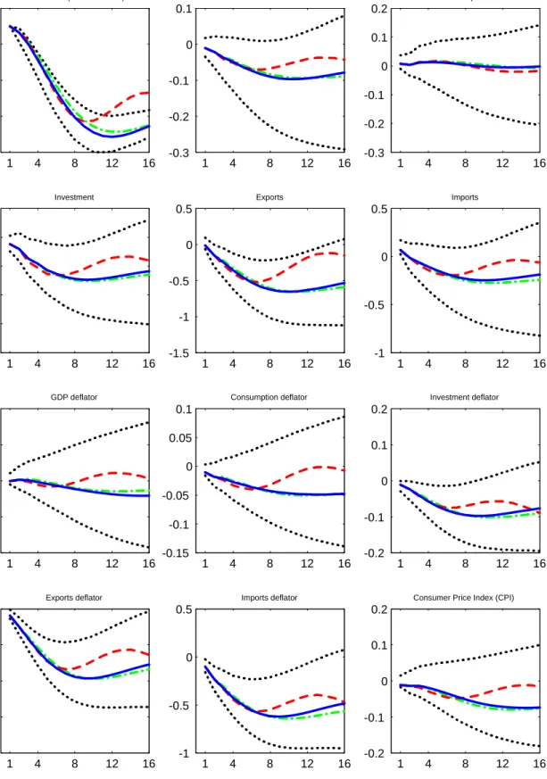
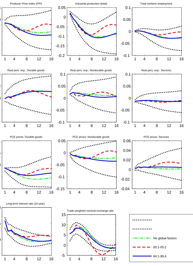
Figures 3 and 4 show the estimated impulse responses of a set of macroeconomic indicators to a tightening of monetary policy, that is, an innovation in the Federal funds rate corresponding to an unexpected increase of 25 basis points. The solid lines represent the responses computed using the relationship between the US factors and the international factors as estimated during the 1984:1 to 1999:4 period, along with the 70% confidence intervals.13 The dashed lines, instead, display the responses using the same FAVAR, but assuming that the US and international factors relate as estimated after 2000. A comparison of these two sets of impulse responses allows us to gauge the effects on the monetary transmission mechanism of the changes in the relationship between international factors and US variables. In fact, between the two sets of responses, the only relationships that are allowed to change are those that describe how foreign factors end up affecting US data. Note that by doing so, we maximize the length of our sample in the estimation, yet we allow for a change in the role of international factors.
As the impulse responses based on the effects of international factors estimated for the 1984:1 - 1999:4 sample reveal in Figures 3 and 4, an unexpected tightening in monetary policy results in a gradual decline in real GDP, which tends to revert back to the original level after about 3 years. Other measures of activity, such as industrial production and employment both respond in a similar way. Consumption also shows a similar although smaller response, while investment falls much more. Together with the fall in domestic demand, imports fall in response to the interest rate increase. The reduction in imports appears to be reinforced by a significant appreciation in the value of the US dollar, lasting about 2 years following the shock. Exports to the rest of the world also fall significantly following the monetary tightening. This is consistent with the fact that the US dollar appreciates, and that output in foreign trade partners falls (not reported).
All price indices (reported in levels) show little response on impact, but also tend to fall pro-1 3The confidence intervals were obtained using Kilian’s (1998) bootstrap procedure.
1 4 8 12 16 -10 0 10 20 30
Interest rate (Federal Funds)
1 4 8 12 16 -0.3 -0.2 -0.1 0 0.1 GDP 1 4 8 12 16 -0.3 -0.2 -0.1 0 0.1 0.2 Consumption 1 4 8 12 16 -2 -1.5 -1 -0.5 0 0.5 Investment 1 4 8 12 16 -1.5 -1 -0.5 0 0.5 Exports 1 4 8 12 16 -1 -0.5 0 0.5 Imports 1 4 8 12 16 -0.1 -0.05 0 0.05 0.1 GDP deflator 1 4 8 12 16 -0.15 -0.1 -0.05 0 0.05 0.1 Consumption deflator 1 4 8 12 16 -0.2 -0.1 0 0.1 0.2 Investment deflator 1 4 8 12 16 -0.8 -0.6 -0.4 -0.2 0 Exports deflator 1 4 8 12 16 -1 -0.5 0 0.5 Imports deflator 1 4 8 12 16 -0.2 -0.1 0 0.1 0.2
Consumer Price Index (CPI)
1 4 8 12 16 -0.15 -0.1 -0.05 0 0.05
Producer Price Index (PPI)
1 4 8 12 16 -0.2 -0.15 -0.1 -0.05 0 0.05
Industrial production (total)
1 4 8 12 16 -0.1 -0.05 0 0.05 0.1
Total nonfarm employment
1 4 8 12 16 -0.4 -0.2 0 0.2 0.4
Real pers. exp.: Durable goods
1 4 8 12 16 -0.1 -0.05 0 0.05 0.1
Real pers. exp.: Nondurable goods
1 4 8 12 16 -0.1 -0.05 0 0.05 0.1
Real pers. exp.: Services
1 4 8 12 16 -0.1 -0.05 0 0.05 0.1
PCE prices: Durable goods
1 4 8 12 16 -0.15 -0.1 -0.05 0 0.05
PCE prices: Nondurable goods
1 4 8 12 16 -0.04 -0.02 0 0.02 0.04 0.06
PCE prices: Services
1 4 8 12 16
-5 0 5 10
Long-term interest rate (10-year)
1 4 8 12 16 -5 0 5 10 15
Trade-weighted nominal exchange rate
No global factors 00:1-05:2 84:1-99:4
gressively, and in a persistent way, following the monetary tightening. However, while the import and export price deflators seem to respond rapidly to the shock, it takes about 3 quarters for the GDP deflator and the CPI to show any movement. While the import price response may reflect a slowing domestic economy, the response of export prices may be explained by a drop in foreign demand for US goods, due both to an appreciating US dollar and to a slowing foreign economy.
4.4
Has the role of global forces on the US monetary transmission changed?
We find little overall evidence that global forces have had a important effect on the US monetary transmission mechanism, andfind little evidence of change over the last several years. To determine to what extent the response of macroeconomic variables to a monetary tightening has changed re-cently, we compare the impulse responses based on the FAVAR involving the link between domestic and international factors as estimated since 2000 (dashed lines) to those based on international factors in the 1984-1999 period (solid lines). One interesting conclusion that emerges from this exercise is that the variables display in both cases almost identical responses in the first 6 to 7 quarters following the shock. After that, the responses based on the most recent international factors reveal a slightly more rapid return to the initial level. The output and various measures of prices, for instance, show less persistent responses to the monetary tightening. But most changes are not statistically significant. Only for the Federal funds rate, the long-term interest rate and the exchange rate do we have sharper evidence that the impulse responses have changed after 3 or 4 years, when using the more recent factors. And the expectation of a higher Federal funds rate three or more years following the shock is reflected in a slightly higher value of the 10-year yield.The changes in the impulse responses just documented were obtained by allowing a different relationship between the US and international factors starting in the year 2000. For robustness, we checked with alternative brea