When Does Direct Real Estate Improve Portfolio
Performance?
Stephen L. Lee
The University of Reading Business School, Centre for Real Estate Research (CRER),
The University of Reading, Reading.
RG6 6AW England
Phone: +44 118 378 6338, Fax: +44 118 378 8172, E-mail: [email protected] Abstract
For over twenty years researchers have been recommending that investors diversify their portfolios by adding direct real estate. Based on the tenets of modern portfolio theory (MPT) investors are told that the primary reason they should include direct real estate is that they will enjoy decreased volatility (risk) through increased diversification. However, the MPT methodology hides where this reduction in risk originates. To over come this deficiency we use a four-quadrant approach to break down the co-movement between direct real estate and equities and bonds into negative and positive periods. Then using data for the last 25-years we show that for about 70% of the time a holding in direct real estate would have hurt portfolio returns, i.e. when the other assets showed positive performance. In other words, for only about 30% of the time would a holding in direct real estate lead to improvements in portfolio returns. However, this increase in performance occurs when the alternative asset showed negative returns. In addition, adding direct real estate always leads to reductions in portfolio risk, especially on the downside. In other words, although adding direct real estate helps the investor to avoid large losses it also reduces the potential for large gains. Thus, if the goal of the investor is offsetting losses, then the results show that direct real estate would have been of some benefit. So in answer to the question when does direct real estate improve portfolio performance the answer is on the downside, i.e. when it is most needed.
When Does Direct Real Estate Improve Portfolio Performance? Introduction
For over twenty years researchers have been recommending that investors diversify their portfolios by adding direct real estate (see Seiler et al, 1999 and Hoesli et al, 2001 for comprehensive reviews). Supported by extensive research that has proclaimed the risk reduction advantages of direct real estate in the mixed-asset portfolio, increasing numbers of institutional investors are adding real estate to their portfolios. Based on the tenets of modern portfolio theory (MPT) investors are told that the primary reason they should include direct real estate is that they will enjoy decreased volatility (risk) through increased diversification. Indeed, it is sometimes claimed that including direct real estate can even boost total portfolio returns (Byrne and Lee, 2003). However, risk reduction remains the primary reason for considering adding direct real estate to an existing portfolio. But when does a holding in direct real estate contribute this increase in portfolio performance?
Traditionally most analysis considers the correlation between direct real estate and the alternative asset classes in examining the risk reducing benefits of adding property to increase diversification. However, the overall correlation coefficient is an average of a large number of concurrent asset movements in many economic and financial environments. Thus, previous studies that have advocated diversification through adding direct real estate to another asset class are essentially assuming that the risk and return characteristics of the various assets are the same even in periods of positive and negative returns. Hence, traditional methods of portfolio analysis based on long run correlation averages fail to identify in which periods real estate helps to reduce portfolio risk. To examine this issue in more depth we break the returns into positive and negative periods to isolate where the benefits between direct real estate and other asset classes originates.
The results suggest that for 70% of the time direct real estate would have contributed little to the return performance of alternative assets. In others words, returns from direct real estate only offset the losses in the alternative asset about 30% of the time. However, this increase in performance occurs when the alternative asset showed negative returns. In addition, adding direct real estate always leads to reductions in portfolio risk, especially downside risk.
The remainder of the paper is structured as follows. The next section gives details of the data and methodology used. The third section presents the results of the four quadrants analysis. Section four examines the impact on risk and return from adding direct real estate to the alternative assets. The final section presents the conclusions.
Data and Methodology
This study examines the risk and return effects that would have been realised by a hypothetical investor who elected to add direct real estate to their existing assets. The assets are equities, bonds and a 60/40-equity/bond portfolio, as most investors will have an existing portfolio of these assets rather than being invested exclusively in one asset class. The returns of equities are represented by the FTA index, government bonds represented by 5-15 year
Gilts and direct real estate is measured by the JLL Index, over the period 1977:Q4 to 2002:Q31 a total of 100 observations.
Using direct real estate data raises the issue of how to deal with the so-called “smoothing bias” observed in appraisal based property indices, see Fisher, et al (1994) and Corgel and deRoos (1999) for comprehensive reviews. While, research is divided as to whether smoothing bias exists and whether it can be appropriately corrected, it seems that the issue is of more concern when comparing direct real estate with market based securities. To account for such appraisal bias and to make the appraisal-based real estate data more comparably with the market based equity and bond returns the real estate data was de-smoothed. The approach adopted here is to use the model suggested by Geltner (1993). However, it should be noted that no de-smoothing process is perfect and the choice of method may bias the results.
Means and standard deviations (SD) are calculated to provide a relative comparison of the different asset classes on both a risk and return basis. Correlation coefficients are then calculated to describe the co-movement between each asset class. The asset with the lowest correlation would usually be a good candidate for risk reduction in a portfolio through increased diversification. The summary statistics are shown in Table 1.
Table 1: Summary Statistics: Quarterly Data 1977:4: to 2002:3
The average quarterly return and SD for each of the three assets and direct real estate are presented in Panel A of Table 1. As observed in Panel A of Table 1 equities offered the highest returns compensating investors for the highest risk. Direct real estate, as represented by the JLL index, showing the lowest risk even after de-smoothing. Panel B of Table 1 shows the correlation coefficients between the asset classes. The correlation between the three assets and direct real estate are all about zero and significantly lower than that between equities and bonds (0.44). Consequently adding direct real estate to these assets should significantly reduce portfolio risk.
Most analysis stops with the correlation between asset classes in explaining the advantages of adding direct real estate to other assets in order to reduce risk. However, although correlation coefficients are an important component of MPT, too few investors appreciate the implications of the co-movement between investments that leads to the correlation between assets. In order to analyse the impact of direct real estate on the performance of other assets more thoroughly we break down the imperfect correlation between direct real estate and the other asset classes to illustrate where the benefits originate. That is in this study we report on the four possible outcomes that can occur when an investor invests in both direct real estate and the other asset classes. The four possible outcomes are:
Panel A Statistics JLL FTA Gilts Port
Mean 2.89 3.60 3.00 3.36
SD 4.37 8.73 5.62 6.55
Panel B Correlation JLL FTA Gilts Port
JLL 1.00
FTA 0.05 1.00
Gilts -0.07 0.44 1.00
2. both markets are down (DD)
3. the asset is up and real estate is down (UD), and 4. the asset is down and real estate is up (DU).
In under taking such an approach a target τ return is required. The target τ is normally set to the minimum return that the investor would be willing to accept this is typically the risk-free rate on T-Bills. Alternatively the target τ could be set to zero: i.e. negative returns are to be avoided. If the minimum target is the performance of some benchmark index, say B that the fund manager is expected to outperform we can define a new variable as the differential performance between the returns of the fund and the benchmark (R-B) and set the target to zero. In other words, a target of zero can be considered as a general case and is the value used here.
Results
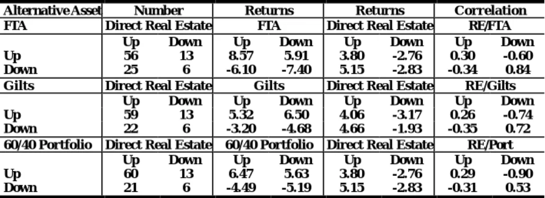
Table 2 presents an analysis of the relationship between the direction of movement of the three assets and direct real estate. Columns 2 and 3 of Table 2 shows the number of times (%) direct real estate and the alternative asset appear in each of the four quadrants. The average returns of the two investments are shown in columns 4 to 7. The last two columns (8 and 9) show the correlation coefficients between direct real estate and the asset2. By using a four-quadrant table for each asset, it is possible to see to what extent the investor really gains from holding direct real estate when it is most needed, i.e. where losses in the asset class are offset by gains in direct real estate.
Table 2: The Number of Periods (%)3 when the Asset Class is Up or Down While Direct Real Estate is Up or Down: Quarterly Data 1977:4 to 2002:3
The first asset class that is reported in Table 2 is equities. In the first quadrant (UU) of the equity data, one may observe that both the FTA index and the JLL index have positive returns. Investing in direct real estate would have done little for an investor holding equities in these 56 periods as direct real estate showed average returns (3.80%) considerably lower than the return in shares (8.57%). In the next quadrant (UD) of Table 2 we observe that in 13 periods, equities showed positive returns (5.91%) and so at least offset the losses in the direct real estate market (-2.76%). In these cases investing in direct real estate clearly hurts
2
The covariances and standard deviations needed to calculate the four quadrant correlation coefficients are calculated as deviations from the overall means. The reason is that we want to compare the four correlations with respect to a common mean. This procedure also guarantees that the correlation of the full sample falls between the positive and negative values.
3
As the total number of periods is one hundred the numbers in Table 2 are also percentages.
Alternative Asset Number Returns Returns Correlation
FTA Direct Real Estate FTA Direct Real Estate RE/FTA
Up Down Up Down Up Down Up Down
Up 56 13 8.57 5.91 3.80 -2.76 0.30 -0.60
Down 25 6 -6.10 -7.40 5.15 -2.83 -0.34 0.84
Gilts Direct Real Estate Gilts Direct Real Estate RE/Gilts
Up Down Up Down Up Down Up Down
Up 59 13 5.32 6.50 4.06 -3.17 0.26 -0.74
Down 22 6 -3.20 -4.68 4.66 -1.93 -0.35 0.72
60/40 Portfolio Direct Real Estate 60/40 Portfolio Direct Real Estate RE/Port
Up Down Up Down Up Down Up Down
Up 60 13 6.47 5.63 3.80 -2.76 0.29 -0.90
portfolio returns compared with investing solely in equities. Hence, we observe for that almost 70% of the time adding direct real estate would probably have resulted in lower portfolio returns.
At the other extreme when both equities and direct real estate showed negative returns (DD) we observe that in 6 periods of the observations adding direct real estate (-2.83%) would have at least decreased the losses in the equity market (-7.40%). Finally, we observe the remaining quadrant of Table 2 (DU). This quadrant represents the occasions in the study period when equities showed negative returns and the direct real estate market positive performance. There are only 25 observations in this quadrant, yet this quadrant represents the situation when direct real estate (5.15%) would have clearly offset the losses in the equity market (-6.10%). Adding these observations to the previously discussed data, we observe that for only about 30% of the time would a holding real estate probably lead to improvements in portfolio returns. However, this improvement in performance occurs when the alternative asset showed negative returns. Thus, if the goal of the investor is offsetting losses, then the results show that direct real estate may have been of some benefit.
Examining Table 2 further to observe the four quadrants for each of the other assets, we see that the pattern is basically the same in each case. The number of periods when a holding in direct real improved the negative performance of bonds and the 60/40-equity/bond portfolio (Port) is 28% and 27% respectively. Thus, direct real estate would have proved detrimental to returns for 72% and 73% of the time. Nonetheless, adding direct real estate to each of the alternative asset classes will always reduce portfolio risk as the correlation coefficients between direct real estate and all assets are all less than one in each quadrant.
Finally, comparing the correlation coefficients shown in Panel B of Table 1 to the results in Table 2 showing the number of observations in the (DU) quadrant for each asset, no distinct pattern is discernible. Low correlation between the various asset classes and direct real estate does not clearly indicate what may be expected in the DU quadrant in Table 2. For example, the 60/40-equity/bond portfolio has the second lowest correlation with direct real estate (0.02), but the lowest number of observations in the DU quadrant (20). Thus, data in the four quadrants provides information that is not clearly ascertained from the use of a single correlation coefficient.
The Impact on Risk and Return
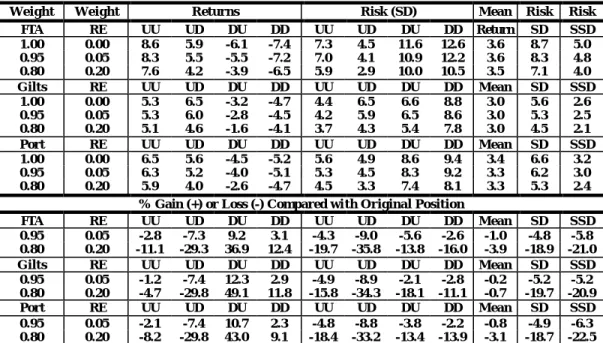
The results of the four-quadrant analysis in Table 2 indicates that adding direct real estate to the other assets improves portfolio returns when the asset shows negative returns, but this is for only about 30% of the time. In other words, a holding in direct real estate would have proved detrimental to performance 70% of the time. Thus, adding direct real estate to another asset class will probably lower overall returns, but may increase returns when it is most needed, i.e. when the alternative asset shows negative performance. In addition, the results in Table 2 show that adding real estate to the other asset should result in lower portfolio risk especially on the downside. In order to test this hypothesis we proceed by adding a holding in direct real estate of 5%, 10%, 15% and 20% to the three assets and calculating the risk and return of the resultant portfolio in the four quadrants used previously.
Table 3 shows that adding 5% property to an equity portfolio leads to a reduction average returns of only 1%, which is more than compensated for by a reduction in risk (SD) of 4.8% and especially downside risk (SSD) of 5.8%. When 20% in property is added to an equity portfolio the reduction in average returns is still only 3.9% for a reduction in risk of 18.9% and 21% in SD and SSD respectively. A similar conclusion can be seen when direct real estate is added to bonds (Gilts) and the 60/40-equity/bond portfolio, with the minor falls in return more than offset by the major reductions in risk.
Table 3: The Benefits of Adding Direct Real Estate to an Existing Equity, Bond and an Equity/Bond Portfolio
The results for a holding of 10% and 15% are not shown for brevity.
Further examination of Table 3 shows that most of the benefit comes when the asset class shows negative returns, as was expected. For instance, when a 20% holding in direct real estate is added to an equity portfolio, when equities have negative returns while direct real estate is showing positive performance (DU) the gain (reduction in loss) in return is 36.9%. Even in the worst case when both markets are showing negative performance there is a reduction in the loss for the portfolio of 12.4%. In contrast, when the equity market is doing well adding 20% direct real estate to an equity portfolio, when real estate shows positive/negative returns, hurts performance by 11.1% and 23.9% respectively. Looking at columns 7 to 10 we find that adding direct real estate to any of the three assets always leads to fall in risk (SD)4 in every quadrant. For instance, adding 20% direct real estate to equities leads to falls in risk of 19.7% (UU) and 35.8% (UD) on the upside, but 13.8% (DU) and 16.0% (DD) on the downside. A similar conclusion can be made when real estate is added to Gilts or a 60/40-equity/bond portfolio. In other words, direct real estate reduces the upside potential of asset classes but compensates the investor by reducing risk.
4
The SD in each of the four quadrants is calculated as deviations from the overall means.
Weight Weight Returns Risk (SD) Mean Risk Risk
FTA RE UU UD DU DD UU UD DU DD Return SD SSD 1.00 0.00 8.6 5.9 -6.1 -7.4 7.3 4.5 11.6 12.6 3.6 8.7 5.0 0.95 0.05 8.3 5.5 -5.5 -7.2 7.0 4.1 10.9 12.2 3.6 8.3 4.8 0.80 0.20 7.6 4.2 -3.9 -6.5 5.9 2.9 10.0 10.5 3.5 7.1 4.0 Gilts RE UU UD DU DD UU UD DU DD Mean SD SSD 1.00 0.00 5.3 6.5 -3.2 -4.7 4.4 6.5 6.6 8.8 3.0 5.6 2.6 0.95 0.05 5.3 6.0 -2.8 -4.5 4.2 5.9 6.5 8.6 3.0 5.3 2.5 0.80 0.20 5.1 4.6 -1.6 -4.1 3.7 4.3 5.4 7.8 3.0 4.5 2.1 Port RE UU UD DU DD UU UD DU DD Mean SD SSD 1.00 0.00 6.5 5.6 -4.5 -5.2 5.6 4.9 8.6 9.4 3.4 6.6 3.2 0.95 0.05 6.3 5.2 -4.0 -5.1 5.3 4.5 8.3 9.2 3.3 6.2 3.0 0.80 0.20 5.9 4.0 -2.6 -4.7 4.5 3.3 7.4 8.1 3.3 5.3 2.4
% Gain (+) or Loss (-) Compared wi th Original Position
FTA RE UU UD DU DD UU UD DU DD Mean SD SSD 0.95 0.05 -2.8 -7.3 9.2 3.1 -4.3 -9.0 -5.6 -2.6 -1.0 -4.8 -5.8 0.80 0.20 -11.1 -29.3 36.9 12.4 -19.7 -35.8 -13.8 -16.0 -3.9 -18.9 -21.0 Gilts RE UU UD DU DD UU UD DU DD Mean SD SSD 0.95 0.05 -1.2 -7.4 12.3 2.9 -4.9 -8.9 -2.1 -2.8 -0.2 -5.2 -5.2 0.80 0.20 -4.7 -29.8 49.1 11.8 -15.8 -34.3 -18.1 -11.1 -0.7 -19.7 -20.9 Port RE UU UD DU DD UU UD DU DD Mean SD SSD 0.95 0.05 -2.1 -7.4 10.7 2.3 -4.8 -8.8 -3.8 -2.2 -0.8 -4.9 -6.3 0.80 0.20 -8.2 -29.8 43.0 9.1 -18.4 -33.2 -13.4 -13.9 -3.1 -18.7 -22.5
Conclusions
The tenets of MPT show investors how to minimise volatility (risk) around a given expected return. Based on this approach a large volume of research has shown that adding direct real estate to the other asset classes leads to significant reductions in portfolio risk. However, the MPT methodology hides where this reduction in risk originates. To over come this deficiency we use a four-quadrant approach to break down the co-movement between direct real estate and equities and bonds into negative and positive periods. Then using data for the last 25-years we show that for about 70% of the time a holding in direct real estate would have hurt portfolio returns, i.e. when the other assets showed positive performance. In other words, for only about 30% of the time would a holding in direct real estate lead to improvements in portfolio returns. However, this increase in performance occurs when the alternative asset showed negative returns. In addition, adding direct real estate always leads to reductions in portfolio risk, especially on the downside. In other words, although adding direct real estate helps the investor to avoid large losses it also reduces the potential for large gains. Thus, if the goal of the investor is offsetting losses, then the results show that direct real estate would have been of some benefit. So in answer to the question when does direct real estate improve portfolio performance the answer is on the downside, i.e. when it is most needed.
References
Byrne, P and Lee S. (2003) The Impact of Real Estate on the Terminal Wealth on the UK Mixed-asset Portfolio, Department of Real Estate and Planning, Working paper 05/03
Fisher, J.D., Geltner, D.M. and Webb, R.B. (1994) Value Indices of Commercial Real Estate: A Comparison of Index Construction Methods, Journal of Real Estate Finance and Economics, 9, 137-164
Geltner, D.M. (1993) Estimating Market Values from Appraised Values without Assuming an Efficient Market, Journal of Real Estate Research, 8, 325-345
Corgel, J.B. and deRoos, J.A. (1999) Recovery of Real Estate Returns for Portfolio Allocation, Journal of Real Estate Finance and Economics, 18, 279-296
Hoesli, M., MacGregor, B., Adair, A. and McGreal, S. (2001) The Role of Property in Mixed Asset Portfolios (MAPs), RICS Foundation, RS0201
Seiler, M.J., Webb, J.R. and Myer, F.C.N. (1999) Diversification Issues in Real estate Investment, Journal of Real Estate Literature, 7, 2, 163-179