Date of publication xxxx 00, 0000, date of current version xxxx 00, 0000. Digital Object Identifier 10.1109/ACCESS.2017.DOI
Multi-scale Residual Hierarchical Dense
Networks for Single Image
Super-Resolution
CHUANGCHUANG LIU1, XIANFANG SUN2, CHANGYOU CHEN3, PAUL L. ROSIN2, YITONG
YAN1, LONGCUN JIN1(Member, IEEE), XINYI PENG1
1
School of Software Engineering, South China University of Technology, Guangzhou, China
2
School of Computer Science and Informatics Cardiff University, UK
3
Department of Computer Science and Engineering, University at Buffalo, State University of New York, NY, USA Corresponding author: Longcun Jin (e-mail: [email protected]).
ABSTRACT Single image super-resolution is known to be an ill-posed problem, which has been studied for decades. With the developments of deep convolutional neural networks, the CNN-based single image super-resolution methods have greatly improved the quality of the generated high-resolution images. However, it is difficult for image super-resolution to make full use of the relationship between pixels in low-resolution images. To address this issue, we propose a novel multi-scale residual hierarchical dense network, which tries to find the dependencies in multi-level and multi-scale features. Specially, we apply the atrous spatial pyramid pooling, which concatenates multiple atrous convolutions with different dilation rates, and design a residual hierarchical dense structure for single image super-resolution. The atrous-spatial-pyramid-pooling module is used for learning the relationship of features at multiple scales; while the residual hierarchical dense structure, which consists of several hierarchical dense blocks with skip connections, aims to adaptively detect key information from multi-level features. Meanwhile, dense features from different groups are connected in a dense approach by hierarchical dense blocks, which can adequately extract local multi-level features. Extensive experiments on benchmark datasets illustrate the superiority of our proposed method compared with state-of-the-art methods. The super-resolution results on benchmark datasets of our method can be downloaded from https://github.com/Rainyfish/MS-RHDN, and the source code will be released upon acceptance of the paper.
INDEX TERMS Convolutional neural networks, deep learning, multi-scale residual hierarchical dense, image super-resolution
I. INTRODUCTION
S
INGLE image super-resolution (SISR) aims torecon-struct a high-resolution (HR) image from its low-resolution (LR) version. Image super-low-resolution is widely used in many computer vision fields, such as video surveil-5
lance, remote sensing, and image sensing. However, SISR is a typically ill-posed problem as the image degradation process is usually irreversible and lots of tiny textures are missing in LR images. Several high-resolution images can be potentially generated from a given LR image. Recently, 10
deep convolutional neural networks have been applied in many tasks, ranging from low-level (image restoration, SISR, etc.) to high-level (image classification, object detection, etc.) vision fields, and have shown great improvements compared
with conventional methods. 15
Currently, CNN-based SISR methods, which learn an ef-fective nonlinear mapping function from LR images to HR images directly, have greatly improved the quality of the super-resolved image. Among them, Dong et al. [1] firstly
used a deep convolutional neural network called SRCNN, 20
consisting of three convolutional layers, to address the SISR problem. Since then, lots of deep-learning SISR methods have been developed. VDSR [2] provides remarkable per-formance by increasing the depth of the network to 20,
proving the importance of the network depth for detecting 25
effective features of images. SRCNN and VDSR involve the interpolated images for pre-processing, whose spatial size is the same as the HR images. FSRCNN [3] was proposed to
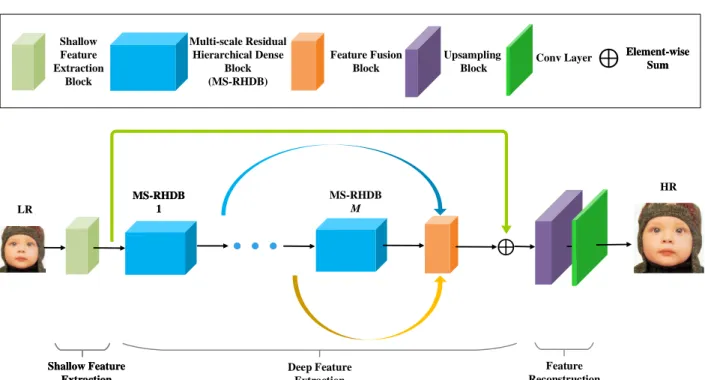
MS-RHDB M Shallow Feature Extraction Shallow Feature Extraction Deep Feature Extraction Feature Reconstruction MS-RHDB 1 MS-RHDB 1 LR HR Multi-scale Residual Hierarchical Dense Block (MS-RHDB) Element-wise Sum Element-wise Sum Feature Fusion Block Shallow Feature Extraction Block Upsampling Block Conv Layer
FIGURE 1.The main architecture of our proposed multi-scale residual hierarchical dense network (MS-RHDN). The blue and yellow arrows denote dense connections, while the green arrow denotes a shortcut connection. The MS-RHDB component is detailed below.
extract features from original LR images and then upscale the spatial size at the end of the network by a deconvolu-30
tional layer. Extracting features directly in LR images instead of interpolated images reduces computations greatly, which becomes a major choice of image super-resolution. LapSRN [4] progressively reconstructs super-resolved images with increasing scales of input images and its improved version 35
MS-LapSRN [5] handles the multiple upsampling scales in one single model. Lim et al. applied a simplified ResNet [6] architecture by removing the unnecessary batch normaliza-tion layer to build a wide network EDSR [7] and a multi-scale deep one MDSR, which won the NTIRE2017 Super-40
Resolution Challenge [8]. Tai et al. [9] proposed recursive and residual learning based DRRN to reduce model parame-ters.
All these methods try to make full use of image infor-mation or features to improve performance, which include 45
increasing the network depth, widening channels, or applying recursive learning. However, most CNN-based SISR models do not take full advantage of the multi-level information from different convolutional layers. Furthermore, these methods usually neglect to use the information from different scales. 50
Objects in images may be similar at different scales and information from different scales may give some clues to help generate high-quality HR images.
To address this issue, we propose a novel network based on the multi-scale structure and residual hierarchical dense 55
connection. The dense connection extracts more information from different layers. We use two levels of dense connections to detect local and global multi-level features. To extract
multi-scale features, we simply apply the residual atrous-spatial-pyramid-pooling structure to fully make use of the 60 information from multiple scales in the LR images. For stabilizing the network and easing the training difficult, we use residual learning to detect more informative features.
Overall, the main contributions of our method are
three-fold: 65
• We propose a unified framework multi-scale residual
hierarchical dense network for image super-resolution. Our method aims at making full use of multi-scale and multi-level features in the LR input image.
• We propose a residual hierarchical dense module to 70
focus on global and local multi-level features. We use sub-dense blocks (SDBs) to adaptively obtain the es-sential parts of the dense features. Skip connections are applied for efficient network training and performance
improvements. 75
• We propose a residual multi-scale structure to detect multi-scale features, which can be readily applied to other super-resolution networks. Such multi-scale struc-ture further improves the performance of the network. In addition, our model obtains much better SR perfor- 80 mance than previous CNN-based methods.
The remainder of this paper is organized as follows: Sec-tion 2 introduces related work on image super-resoluSec-tion. Section 3 presents the proposed method. Section 4 gives experimental results on benchmark datasets. Visual compar- 85 isons with other methods are also included. To show the effectiveness of the components in our network, Section 5 gives the network investigations. Finally, Section 6 draws
conclusions.
II. RELATED WORK
90
The SISR methods can mainly be categorized into
three classes: interpolation-based methods [10]–[13],
reconstruction-based methods [14]–[16], and learning-based methods. The interpolation-based methods, such as bilinear interpolation and bicubic interpolation, are simple and fast, 95
but suffer from over-smoothed textures and thus are not able to produce high-quality images. The reconstruction-based methods are flexible and usually use prior knowledge to produce high-frequency details. However, these methods are usually time-consuming and suffer from rapid degeneration 100
of performance with the increasing upsampling factor. The learning-based methods attempt to learn mappings from LR space to HR space directly. Freeman et al. [17] firstly used Markov random fields (MRF) to generate syn-thetic images, where the parameters of the model are learned 105
from the examples. Chang et al. [18] used locally linear embedding (LLE) [19] to find the resolutions from the linear combination of nearest neighbors. ANR [20] proposed by Timofte et al. uses sparse learned dictionaries and applies the coefficients calculated from LR patches to the corresponding 110
SR patches directly. A+ [21], an improved version of ANR, learns regressors on all training patches. There also exist SR methods based on decision trees or random forests such as [22]–[26] to address the SISR problem.
Recently, deep-learning based methods have shown great 115
improvements in image super-resolution. Specifically, Dong et al. [1] firstly proposed a deep convolutional neural network SRCNN for the SISR problem. The depth of the network plays an important role in many vision tasks, Kim et al. proposed VDSR [2] with remarkable performance, which 120
increased the depth of the network. To reduce the parame-ters and find the dependencies of different proceeding time, DRRN [9] uses recursive learning and the memory block with the deeper network. Instead of interpolating the original LR images to the desired size before putting them into the 125
networks, FSRCNN [3] extracted features from the original LR images and used a deconvolutional layer to upscale the spatial size at the end of the network, which greatly reduced the computations. This manner is commonly used in recent SR methods. LapSRN [4] progressively reconstructs 130
the HR image with increasing scales of input images. MS-LapSRN [5], an improved version of MS-LapSRN, uses a multi-scale training strategy to handle the multiple upsampling scales in one single model. Shi et al. [27] proposed ESPCN, which introduces a sub-pixel convolutional layer for efficient 135
upsampling. Lim et al. [7] proposed EDSR and a multi-scale deep MDSR, which removed the unnecessary batch normal-ization layer from the ResNet [6] architecture. SRMDNF [28] is proposed to handle multiple degradations by concatenating degradation maps and images as the input to the network 140
and adaptively learn to produce high-quality images under different blur kernels of downsampling. ZSSR [29] (zero-shot super-resolution) uses an unsupervised approach to learn
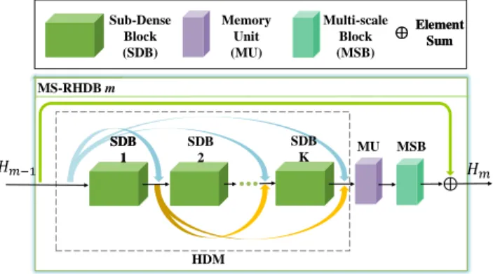
MS-RHDB m MS-RHDB m MS-RHDB m SDB 2 SDB K SDB 1 SDB 1 Sub-Dense Block (SDB) Memory Unit (MU) Element Sum Element Sum Multi-scale Block (MSB) HDM MU MSB
FIGURE 2.Multi-scale residual hierarchical dense block (MS-RHDB).
the mapping from LR images to HR images, whose training
data are generated by downsampling the test data. D-DBPN 145
[30] uses an error-correcting feedback mechanism for SR by iterative up and downsampling. RDN [31] proposed by Zhang et al. uses residual and dense connections and achieves state-of-the-art performance. Zhang et al. [32] proposed RNAN, where local and non-local attention blocks are used 150 to adaptively rescale features with soft attention.
In order to produce photo-realistic SR images, Ledig et al. [33] firstly introduced residual learning and generative adversarial network (GAN) to decrease the distance between
the distributions of real images and SR images. However, 155
the images generated by SRGAN still contain noise and artifacts. Wang et al. [34] introduced an enhanced SRGAN, which applied relativistic GAN [35] to the discriminator and adopted residual scaling [36], smaller initialization, and net-work interpolation, to remove artifacts and won the first place 160 in the 2018 PIRM-SR challenge in region 3. For producing realistic SR images, many loss functions have been proposed. The perceptual loss [37] is proposed to reduce the pixel-wise distances of high-level features produced by pre-trained models, e.g. VGG19 [38]. Contextual loss [39] maintains the 165 image statistics and approximates the KL-divergence.
Making full use of the information in the LR images is the key to produce plausible SR images. To investigate multi-scale and multi-level features, we propose a multi-scale residual hierarchical dense network to obtain results with 170 improvements in quality and quantity. We will introduce our method in the next section.
III. PROPOSED METHOD
In this paper, our method aims to reconstruct a high-resolution image ISR ∈ RW r×Hr×C from a low-resolution
175
imageILR ∈RW×H×C, whereW andH are the width and
height of the LR image,ris the upscaling factor, andCis the number of channels of the color space. Fig.1 shows the main framework of our network, whose components are detailed
below. 180
A. NETWORK ARCHITECTURE
Our proposed multi-scale residual hierarchical dense network (MS-RHDN) consists of three main components: shallow feature extractionFSF, deep feature extractionFDF, and
fea-ture reconstructionFREC. We use one convolutional layer to
185
extract the shallow features H0, including edges, corners, etc., fromILR:
H0=FSF(ILR), (1)
where H0 is the input to the deep feature extraction mod-ule. In deep feature extraction, we useM sequential multi-scale residual hierarchical dense blocks (MS-RHDB) and a 190
global fusion layer FGF to extract and fuse multi-scale and
multi-level features. Furthermore, a global skip connection is introduced to make the main parts of the network focus on high-frequency information. Formally, we have
HDF =FDF(H0)
=H0+FGF([H1, H2, ..., Hm, ..., HM]) withHm=FMSDm (Hm−1),
(2)
whereFm
MSD denotes the mapping of them-th MS-RHDB;
195
[·]stands for the concatenation operator. Finally, the feature reconstruction module produces a high-resolution imageISR
based on the featureHDF:
ISR=FREC(HDF) =Fconv(Fup(HDF)). (3)
Here the feature reconstruction module is composed of an upscaling layer Fup and a convolutional layerFconv. There
200
have been a number of advanced upsampling structures,e.g., deconvolutional layer, sub-pixel convolution, EUSR [40]. Here we adopt the sub-pixel convolution, which has been shown effective in previous works such as EDSR [7] and RDN [31].
205
To define a proper loss function, researchers have de-signed different loss functions such as L2,L1, perceptual, and adversarial losses. In our work, we choose L1 loss in order to reduce computational complexity. Given a training set{ILR
i , IiHR}Ni=1, whereILRis obtained by down-sampling
210
fromIHRwith scaling factorr, theL
1loss is defined as: L1(IiSR, IiHR) = 1 W r×Hr×C × C X c=1 W r X w=1 Hr X h=1 ||Fθ(IiLR)(w, h, c)−I HR i (w, h, c)||1, (4)
whereW,H, andCstand for the width, height, and channels of the low-resolution image respectively andris the scaling factor.Fθ denotes the function of our network andθ stands for the set of parameters, which are updated by stochastic 215
gradient descent.
B. MULTI-SCALE RESIDUAL HIERARCHICAL DENSE BLOCK (MS-RDHB)
The proposed MS-RHDB framework mainly contains three components: a hierarchical dense module, a memory unit, 220
and a multi-scale block. This section details the hierarchical
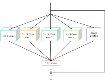
Conv Conv rate=1 Conv rate=2 Conv rate=4 Image pooling Conv
FIGURE 3.Residual multi-scale block (MSB) architecture.
dense module and the memory unit. Detailed description of the multi-scale block is given in Section III-C.
Hierarchical dense module (HDM) The hierarchical dense module is built to adequately exploit multi-level fea- 225 tures. In the module,Ksub-dense blocks (SDB) are arranged in a dense manner. Detailed description of SDB is introduced in Section III-D. In general, an HDM takesHm−1 as input, and outputs an intermediate feature HHDM
m . Formally, this
procedure is described as: 230
HmHDM=F m HDM(Hm−1) =FSDBK ([Hm−1, S1, ..., Sk, ..., SK−1]), (5) where Fm
HDM denotes the function of an HDM in them-th
MS-RHDB block; andFK
SDB denotes the function of theK
-th SDB -that constitutes Fm
HDM.Sk denotes the output of the k-th SDB, whose input is the concatenation of outputs of the
previousk−1SDBs. Formally,Skcan be presented as: 235
Sk=FSDBk ([Hm−1, S1, ..., Sk−1]), (6)
whereFk
SDB denotes the function of thek-th SDB.Sk con-tainsGfeature-maps, whereGis the number of channels and also known as growth rate in [41].
Memory unit. After extracting multi-level features with
a set of SDBs, we use a memory unit [42] to integrate 240
these features, which is supposed to adaptively extract unified information. Furthermore, a memory unit is also useful to reduce the number of feature-maps, thus reducing the number of parameters and computations. Specifically, the memory
unit is defined as: 245
HmMU=FMUm([Hm−1, S1, ..., Sk, ..., SK]), (7)
where Fm
MU denotes the mapping function of the memory
unit in them-th MS-RHDB; andHMU
m is the output ofF m
MU.
Following [9] [31], the memory unit is represented with a 1 ×1 convolutional layer. Finally, we use a multi-scale structure, which will be introduced in section III-C, to extract 250
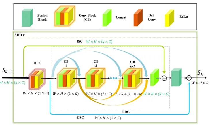
BLC CB 1 CB 2 CB k-1 Conv Block (CB) Concat 3x3 Conv ReLu Fusion Block ISC CSC LDG
FIGURE 4.Network architecture of our proposed sub-dense block (SDB). For a SDB,W×H×(e×G)is the input size of every Conv block (CB), andedenotes the index of the CB. The output size of each CB isW×H×(1×G). “Concat” stands for the concatenation operator, and “3×3Conv” refers to a convolutional layer with the kernel size of
3×3.
features from different scales for taking full advantage of fused features by the memory unit. A skip connection is in-troduced for a similar purpose to the global skip connection. The final output of them-th MS-RHDB is obtained by:
Hm=Hm−1+FMSm(H MU
m ), (8)
whereFm
MS denotes the function of the multi-scale block in
255
them-th MS-RHDB.
C. MULTI-SCALE BLOCK (MSB)
As discussed above, multi-scale information is useful in generating high-quality super-resolution images. In this sec-tion, we elaborate on our multi-scale block used in (8). 260
As shown in Fig.3, the MSB mainly consists of an atrous-spatial-pyramid-pooling (ASPP) structure and a local skip connection.
The ASPP structure is firstly introduced in DeepLabV3 [43] for handling different sizes of objects in street-scene 265
segmentation. ASPP consists of several parallel atrous con-volutional layers with different dilated rates. In our model, we apply ASPP to detect useful components of the fused hierarchical dense features. In addition, to make the network efficient and stable, we add a local skip connection to each 270
ASPP. Formally, our multi-scale block is defined as:
HmMS=HmMU+FASPPm (H MU
m ), (9)
whereFm
ASPP denotes the function of the ASPP structure in
them-th MS-RHDB; andHMS
m denotes the output of them -th MSB.
D. SUB-DENSE BLOCK (SDB) 275
In order to extract local multi-level features, we introduce a sub-dense neural network. As introduced above, an HDM is constructed by stacking several SDBs in a dense man-ner, where SDBs are used to extract local multi-level fea-tures from previous concatenated feafea-tures. Because the input 280 channels of each SDB may be different, the number of convolutional layers is determined by the number of the input feature-maps. More feature-maps need more layers. As shown in Fig.4, SDB contains four components:
bottleneck-like compression (BLC), local dense group (LDG), input 285
shortcut connection (ISC), and compression shortcut connec-tion (CSC).
Firstly, we use a BLC, which is a bottleneck-like method by a3×3Conv layer for reducing parameters and compu-tations. After compressing the number of feature-maps into 290 G, we stack several conv blocks in a manner similar to the DenseNet [41], until the number of feature-maps equals that of the input in LDG. A conv block consists of a concatenation operator applied to all the previous features, a convolutional layer with kernel size of 3 ×3, and an activation layer, 295 as shown in Fig.4. The input of the k-th SDB, Sk, is the concatenation of the outputs of the previousk−1layers and
TABLE 1.Quantitative results with the BI degradation model. The best and second best results arehighlightedand underlined respectively.
Method Scale Set5 Set14 B100 Urban100 Manga109
PSNR SSIM PSNR SSIM PSNR SSIM PSNR SSIM PSNR SSIM
Bicubic ×2 33.66 0.9299 30.24 0.8688 29.56 0.8431 26.88 0.8403 30.80 0.9339 SRCNN [1] ×2 36.66 0.9542 32.45 0.9067 31.36 0.8879 29.50 0.8946 35.60 0.9663 FSRCNN [3] ×2 37.05 0.9560 32.66 0.9090 31.53 0.8920 29.88 0.9020 36.67 0.9710 VDSR [2] ×2 37.53 0.9590 33.05 0.9130 31.90 0.8960 30.77 0.9140 37.22 0.9750 LapSRN [4] ×2 37.52 0.9591 33.08 0.9130 31.08 0.8950 30.41 0.9101 37.27 0.9740 MemNet [42] ×2 37.78 0.9597 33.28 0.9142 32.08 0.8978 31.31 0.9195 37.72 0.9740 EDSR [7] ×2 38.11 0.9602 33.92 0.9195 32.32 0.9013 32.93 0.9351 39.10 0.9773 SRMDNF [28] ×2 37.79 0.9601 33.32 0.9159 32.05 0.8985 31.33 0.9204 38.07 0.9761 D-DBPN [30] ×2 38.09 0.9600 33.85 0.9190 32.27 0.9000 32.55 0.9324 38.89 0.9775 RDN [31] ×2 38.24 0.9614 34.01 0.9212 32.34 0.9017 32.89 0.9353 39.18 0.9780 RNAN [32] ×2 38.17 0.9611 33.87 0.9207 32.32 0.9014 32.73 0.9340 39.23 0.9785 SDNND [44] ×2 38.07 0.9610 33.77 0.9195 32.25 0.9026 32.55 0.9332 – – MS-RHDN (ours) ×2 38.26 0.9615 33.92 0.9206 32.36 0.9020 33.02 0.9367 39.33 0.9781 MS-RHDN+ (ours) ×2 38.31 0.9617 34.01 0.9212 32.40 0.9025 33.24 0.9382 39.50 0.9785 Bicubic ×3 30.39 0.8682 27.55 0.7742 27.21 0.7385 24.46 0.7349 26.95 0.8556 SRCNN [1] ×3 32.75 0.9090 29.30 0.8215 28.41 0.7863 26.24 0.7989 30.48 0.9117 FSRCNN [3] ×3 33.18 0.9140 29.37 0.8240 28.53 0.7910 26.43 0.8080 31.10 0.9210 VDSR [2] ×3 33.67 0.9210 29.78 0.8320 28.83 0.7990 27.14 0.8290 32.01 0.9340 LapSRN [4] ×3 33.82 0.9227 29.87 0.8320 28.82 0.7980 27.07 0.8280 32.21 0.9350 MemNet [42] ×3 34.09 0.9248 30.00 0.8350 28.96 0.8001 27.56 0.8376 32.51 0.9369 EDSR [7] ×3 34.65 0.9280 30.52 0.8462 29.25 0.8093 28.80 0.8653 34.17 0.9476 SRMDNF [28] ×3 34.12 0.9254 30.04 0.8382 28.97 0.8025 27.57 0.8398 33.00 0.9403 RDN [31] ×3 34.71 0.9296 30.57 0.8468 29.26 0.8093 28.80 0.8653 34.13 0.9484 SDNND [44] ×3 34.41 0.9277 30.25 0.8425 29.10 0.8076 28.35 0.8571 – – MS-RHDN (ours) ×3 34.76 0.9302 30.61 0.8475 29.29 0.8104 28.95 0.8681 34.40 0.9497 MS-RHDN+ (ours) ×3 34.82 0.9305 30.71 0.8490 29.34 0.8114 29.16 0.8712 34.69 0.9510 Bicubic ×4 28.42 0.8104 26.00 0.7027 25.96 0.6675 23.14 0.6577 24.89 0.7866 SRCNN [1] ×4 30.48 0.8628 27.50 0.7513 26.90 0.7101 24.52 0.7221 27.58 0.8555 FSRCNN [3] ×4 30.72 0.8660 27.61 0.7550 26.98 0.7150 24.62 0.7280 27.90 0.8610 VDSR [2] ×4 31.35 0.8830 28.02 0.7680 27.29 0.7260 25.18 0.7540 28.83 0.8870 LapSRN [4] ×4 31.54 0.8850 28.19 0.7720 27.32 0.7270 25.21 0.7551 29.09 0.8900 MemNet [42] ×4 31.74 0.8893 28.26 0.7723 27.40 0.7281 25.50 0.7630 29.42 0.8942 EDSR [7] ×4 32.46 0.8968 28.80 0.7876 27.71 0.7420 26.64 0.8033 31.02 0.9148 SRMDNF [28] ×4 31.96 0.8925 28.35 0.7787 27.49 0.7337 25.68 0.7731 30.09 0.9024 D-DBPN [30] ×4 32.47 0.8980 28.82 0.7860 27.72 0.7400 26.38 0.7946 30.91 0.9137 RDN [31] ×4 32.47 0.8990 28.81 0.7871 27.72 0.7419 26.61 0.8028 31.00 0.9151 RNAN [32] ×4 32.49 0.8982 28.83 0.7878 27.72 0.7421 26.61 0.8023 31.09 0.9149 SDNND [44] ×4 32.21 0.8954 28.54 0.7817 27.55 0.7364 26.23 0.7914 – – MS-RHDN (ours) ×4 32.62 0.8998 28.85 0.7881 27.75 0.7424 26.72 0.8059 31.30 0.9179 MS-RHDN+ (ours) ×4 32.70 0.9009 28.97 0.7901 27.81 0.7438 26.92 0.8101 31.62 0.9205 Bicubic ×8 24.40 0.6580 23.10 0.5660 23.67 0.5480 20.74 0.5160 21.47 0.6500 SRCNN [1] ×8 25.33 0.6900 23.76 0.5910 24.13 0.5660 21.29 0.5440 22.46 0.6950 FSRCNN [3] ×8 20.13 0.5520 19.75 0.4820 24.21 0.5680 21.32 0.5380 22.39 0.6730 SCN [45] ×8 25.59 0.7071 24.02 0.6028 24.30 0.5698 21.52 0.5571 22.68 0.6963 VDSR [2] ×8 25.93 0.7240 24.26 0.6140 24.49 0.5830 21.70 0.5710 23.16 0.7250 LapSRN [4] ×8 26.15 0.7380 24.35 0.6200 24.54 0.5860 21.81 0.5810 23.39 0.7350 MemNet [42] ×8 26.16 0.7414 24.38 0.6199 24.58 0.5842 21.89 0.5825 23.56 0.7387 MS-LapSRN [5] ×8 26.34 0.7558 24.57 0.6273 24.65 0.5895 22.06 0.5963 23.90 0.7564 EDSR [7] ×8 26.96 0.7762 24.91 0.6420 24.81 0.5985 22.51 0.6221 24.69 0.7841 D-DBPN [30] ×8 27.21 0.7840 25.13 0.6480 24.88 0.6010 22.73 0.6312 25.14 0.7987 MS-RHDN (ours) ×8 27.13 0.7820 25.13 0.6471 24.89 0.6016 22.76 0.6326 24.94 0.7907 MS-RHDN+ (ours) ×8 27.32 0.7876 25.27 0.6505 24.96 0.6037 22.93 0.6388 25.21 0.7971 Hm−1, which containsk×Gchannels. As a result, the LDG
in thek-th SDB requiresk−1convolutional layers to reach the same number of channels as that of the input. Formally, 300
the LDG is described as:
SLDGk =FLDGk ([Sk−BLC1, Sk−1,1, ..., Sk−1,d, ..., Sk−1,k−1]), (10) whereSBLC
k−1is the output of BLC, andSk−1,dis the output of thed-th Conv in thek-th SDB.Fk
LDGdenotes the function of
the local dense group in thek-th SDB andSLDG
k is its output. Similarly, the input of thed-th Conv is the concatenation of 305
proceeding layers. In SDB, the local dense group adaptively detects local multi-level features according to the amount of
information that the input has.
ISC andCSC. At the same time, the ISC stands for an element-wise addition in the inputSk−1and the multi-level 310 featuresSk−1,k−1. After that, we apply a1×1Conv to fuse the number of feature-maps into G. Finally, the compressed feature SBLC
k−1 is added to the output of the fusion block by CSC. These two shortcut connections are important for detecting more informative cues and improving performance, 315 as well as stabilizing the network.
E. IMPLEMENTATION DETAILS
In this section, we specify some implementation details of our proposed MS-RHDN. We set the kernel size of all the
Urban100 img_004 HR Bicubic SRCNN [1] FSRCNN [3] VDSR [2] PSNR/SSIM 21.08/0.6788 22.13/0.7635 22.02/0.7628 22.37/0.7939 LapSRN [4] EDSR [7] D-DBPN [42] SRMDNF [28] MS-RHDN 22.41/0.7989 24.07/0.8591 23.74/0.8497 22.92/0.8192 24.88/0.8756 Urban100 img_074 HR Bicubic SRCNN [1] FSRCNN [3] VDSR [2] PSNR/SSIM 22.16/0.5622 22.72/0.6200 22.73/0.6180 23.07/0.6415 LapSRN [4] EDSR [7] D-DBPN [42] SRMDNF [28] MS-RHDN 23.14/0.6520 24.12/0.7362 23.99/0.7234 23.41/0.6752 24.58/0.7606 Urban100 img_092 HR Bicubic SRCNN [1] FSRCNN [3] VDSR [2] PSNR/SSIM 16.57/0.4417 17.55/0.5447 17.70/0.5561 18.14/0.6011 LapSRN [4] EDSR [7] D-DBPN [42] SRMDNF [28] MS-RHDN 18.19/0.6076 18.92/0.6661 18.90/0.6596 18.57/0.6306 19.72/0.6976 Manga109 YumeiroCooking HR Bicubic SRCNN [1] FSRCNN [3] VDSR [2] PSNR/SSIM 24.68/0.7849 26.22/0.8464 26.38/0.8496 26.89/0.8703 LapSRN [4] EDSR [7] D-DBPN [42] SRMDNF [28] MS-RHDN 26.92/0.8739 27.74/0.8972 28.27/0.9079 27.51/0.8897 29.14/0.9256
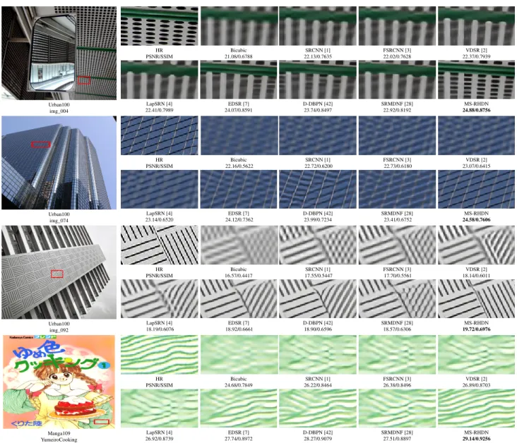
FIGURE 5.Visual comparison for4×SR with the BI model on the Urban100 and Manga109 datasets. The best results arehighlighted.
convolutional layers to 3×3, except for the fusion layers, 320
whose kernel sizes are set to 1 ×1. The number of
MS-RHDB is set to M = 10. In each MS-RHDB, we set the
number of SDBs asK = 5. The number of convolutional
layers in LDG is decided adaptively, depending on the input. As an illustration, the LDG in the k-th SDB stack k −1 325
convolutional layers organized in a dense manner to get the same number of channels as the input. We set the growth rate asG = 64. We use ESPCN [27] to upscale the coarse resolution feature-maps to fine ones in our reconstruction module. At the tail of the network, we use 3 convolutional 330
filters to generate high-quality super-resolved images with 3 color channels.
Difference to RDN. Here, we mainly summarize three differences between our method and the RDN [31]. First, both RDN and our model use dense connections. However, 335
multi-level dense connections are adopted in our MS-RHDN, compared to one level in RDN. Second, we apply
multi-scale blocks to our MS-RHDN, which aims at extracting multi-scale information from features, while RDN ignores this important information. Third, we proposed SDBs to learn 340 local hierarchical features instead of simple convolutional layers in RDN. Experiments in the next section show that our MS-RHDN outperforms RDN in benchmark datasets with less parameters.
IV. EXPERIMENTAL RESULTS 345
In this section, we conduct quantitative and visual compar-isons with several state-of-the-art methods on benchmark datasets under two commonly used image degradations: bicu-bic downsampling and blur-downsampling, respectively.
A. SETTINGS 350
We use the DIV2K dataset [8] as our training set, which
contains 800, 100 and 100 images of 2K-resolution for
training, validation, and testing, respectively. The LR images
TABLE 2.Quantitative results with the blur-down degradation model. Best and second best results arehighlightedand underlined.
Method Scale Set5 Set14 B100 Urban100 Manga109
PSNR SSIM PSNR SSIM PSNR SSIM PSNR SSIM PSNR SSIM
Bicubic ×3 28.78 0.8308 26.38 0.7271 26.33 0.6918 23.52 0.6862 25.46 0.8149 SPMSR [46] ×3 32.21 0.9001 28.89 0.8105 28.13 0.7740 25.84 0.7856 29.64 0.9003 SRCNN [1] ×3 32.05 0.8944 28.80 0.8074 28.13 0.7736 25.70 0.7770 29.47 0.8924 FSRCNN [3] ×3 26.23 0.8124 24.44 0.7106 24.86 0.6832 22.04 0.6745 23.04 0.7927 VDSR [2] ×3 33.25 0.9150 29.46 0.8244 28.57 0.7893 26.61 0.8136 31.06 0.9234 IRCNN [47] ×3 33.38 0.9182 29.63 0.8281 28.65 0.7922 26.77 0.8154 31.15 0.9245 RDN [31] ×3 34.58 0.9280 30.53 0.8447 29.23 0.8079 28.46 0.8582 33.97 0.9465 MS-RHDN (ours) ×3 34.76 0.9292 30.67 0.8468 29.32 0.8098 28.83 0.8648 34.49 0.9491 MS-RHDN+ (ours) ×3 34.82 0.9298 30.75 0.8481 29.32 0.8108 29.04 0.8679 34.78 0.9505
are obtained by bicubic downsampling (BI) from the source high-resolution images. At testing, we use five standard 355
benchmark datasets: Set5 [48], Set14 [49], BSD100 [50], Urban100 [51], and Manga109 [52]. We transform the im-ages into YCrCb color space and evaluate the performance by PSNR and SSIM on the Y channel.
In training, images are augmented by rotating and flipping. 360
The batch size is set to 16. Our MS-RHDN is trained based on image patches and optimized with the ADAM optimizer [53].
The hyperparameters β1 and β2 in the ADAM optimizers
are set to β1 = 0.9 and β2 = 0.999. We randomly crop
48×48patches from LR images as the input of the network. 365
Following [4], [7], [27], [31], [32], the initial learning rate is set to1×10−4, which decays to half every2×105iterations. We implement our model using the Pytorch [54] framework with a Titan Xp GPU. Training the MS-RHDN roughly takes one day with2×105iterations.
370
B. COMPARISONS WITH STATE-OF-THE-ART METHODS We compare our model with 13 state-of-the-art image SR algorithms: SRCNN [1], VDSR [2], FSRCNN [3], SCN [45], LapSRN [4], MemNet [42], EDSR [7], SRMDNF [28], D-DBPN [30], RDN [28], RNAN [32], and SDNND [44]. 375
Similar to [7], [31], [55], we also apply a self-ensemble strategy, which rotates and flips inputs to generate different versions of high-resolution images. The corresponding in-verse transforms are applied to generate an HR image, which is an average version of all the HR images. This version is 380
denoted as the self-ensembled MS-RHDN or MS-RHDN+. Quantitative comparison. Table 1 shows the results of the proposed method and state-of-the-art methods for ×2,
×3,×4, and×8SR. We directly adopt the results of RNAN [32] and SDNND [44]. It can be seen that our MS-RHDN+ 385
performs the best on all the test datasets in most scaling factors by a large margin. The MS-RHDN also outperforms other compared methods even without self-ensemble. This indicates that our network is effective in detecting compre-hensive features for reconstructing tiny textures. Besides, 390
our MS-RHDN obtains larger margins with the increase of scaling factors. We argue that it is more essential to make full use of information in LR images for a large scaling factor. The observations demonstrate that the multi-scale block and residual hierarchical dense structure allow our network to 395
further extract more informative features and improve the
performance.
Qualitative comparison.Next, we qualitatively compare our method with state-of-the-art methods. Fig.5 shows the
visual comparisons of SR images generated by our method 400
and the methods compared. We obtain several observations from Fig.5. For image ‘img_004’ in Urban100, most com-pared methods produce images with blurring artifacts. What is worse, most of them cannot recover the detailed textures of the green horizontal line and lattices. However, our method 405 can generate more tiny textures and remove the artifacts. For image ‘img_074’, we can find that most compared methods cannot generate the horizontal line correctly and also suffer from blurring artifacts. Some of them even produce edges
with wrong directions. By contrast, our MS-RHDN shows 410
great abilities in producing accurate information from the LR image. For image ‘img_092’, we observe that Bicubic, SR-CNN, FSRSR-CNN, VDSR, and LapSRN suffer from blurring artifacts. Even though EDSR, D-DBPN, and SRMDNF can recover some high-frequency information, the right part of 415 the cropped image generated by these methods shows wrong directions of the gap with over-smoothed edges. Our MS-RHDN can be more faithful to the ground truth. For image ‘YumeiroCooking’, due to the abundance of textures, most
compared methods cannot fully recover them and obviously 420
produce blurring artifacts. Our method achieves a better result, which is more similar to the HR image.
Overall, our method shows better performance both quan-titatively and visually, as it provides a nice way to make
full use of features in LR images. Our proposed residual 425
hierarchical dense module successfully detects multi-level features. The multi-scale block is further used to extract information from multiple scales. Multiple residual connec-tions are applied to make the network focus on important parts, and to facilitate the training of the proposed network. 430
Following [31], [47], we further apply our method to recover images from a blur-down degradation model. A high-resolution image is first blurred by a Gaussian kernel, and then downsampled with a scaling factor. The size of the
Gaussian kernel is 7 × 7 with standard deviation of 1.6. 435
We compare our method with 6 state-of-the-art methods: SPMSR [46], SRCNN [1], FSRCNN [3], VDSR [2], IR-CNN [47], and RDN [31]. Table 2 shows the results of our method and the compared methods in terms of PSNR
Urban100 img_046 HR Bicubic RDN [31] MS-RHDN (ours) PSNR/SSIM 22.78/0.6859 25.02/0.8364 25.35/0.8498 HR Bicubic RDN [31] MS-RHDN (ours) PSNR/SSIM 22.78/0.6859 25.02/0.8364 25.35/0.8498 Manga109 MisutenaideDaisy HR Bicubic RDN [31] MS-RHDN (ours) PSNR/SSIM 26.62/0.8884 37.17/0.9800 38.36/0.9816 HR Bicubic RDN [31] MS-RHDN (ours) PSNR/SSIM 26.62/0.8884 37.17/0.9800 38.36/0.9816
FIGURE 6.Visual comparison for3×SR with the BD model. The best results arehighlighted.
TABLE 3.Investigations of HDM (including ISC, CSC, LDG) and MSB. We observe the best PSNR (dB) values on Set5 (4×) in 100 epochs.
Structure 1 2 3 4 5 6 7 8 9
Hierarchical Dense Module (HDM) LDG % % ! ! ! ! ! ! ! ISC % % % ! % ! ! % ! CSC % % % % ! ! % ! ! Multi-Scale Block (MSB) % ! % % % % ! ! ! PSNR on Set5 (4×) 31.50 31.94 31.82 31.87 31.87 31.93 32.01 31.97 32.05
performance on all the benchmark datasets, and MS-RHDN+ achieves the best results. Our methods outperform RDN by a large margin. The observations indicate that the structure MS-RHDN is more efficient and has a stronger ability to recover images from the blur-down degradation model. Fig. 6 445
demonstrates visual comparisons for3×SR under the blur-down degradation model. For image ‘img_046’ in Urban100, it is observed that the two patches generated by Bicubic are totally blurred and lose most details. RDN can recover some details but produces some edges with wrong directions. In 450
contrast, MS-RHDN obtains much better performance with sharper edges and correct structures. However, it can be seen from the left parts of the cropped patches on the first line of Fig. 6 that it is challenging for our method and the RDN to recover tiny textures, as these textures are badly blurred 455
in the input LR image. This problem is also the concern in other single image super-resolution methods. Nevertheless, if we zoom in the picture, we can find that our method can still generate edge effect even in the left part of the cropped patch, while the RDN cannot. For image ‘MisutenaideDaisy’ in 460
Manga109, characters in the two patches produced by Bicu-bic cannot even be recognized by eyeballing. RDN recovers some details of the characters with simple structures,e.g., “c” and “s”. However, some characters in the first patch suffer from blurring artifacts and lose some structures. In com- 465 parison, MS-RHDN can recover more details and maitain the right structures. In the second patch, RDN generates characters with over-smoothed edges and blurring artifacts. In contrast, our MS-RHDN alleviates the over-smoothness and blurring-artifacts issues by recovering sharper edges. It 470 also demonstrates the promising potential to make full use of the multi-level and multi-scale features for SR with a blur-down degradation model.
V. NETWORK INVESTIGATIONS
We show ablation investigations on the hierarchical dense 475 module and the multi-scale block in table 3. The structure 9 has 10 MS-RHDBs (M=10), 5 SDBs (K=5), and growth rate (G=32). We set the batch size to 8 for fast training. To show the superiority of our structure and reduce the influence
0 20 40 60 80 100 Epoch 28.5 29.0 29.5 30.0 30.5 31.0 31.5 32.0 PSNR (dB)
Ablation Investigation of LDG, ISC, CSC, and MSB
LDG1_ISC1_CSC1_MSB1 LDG0_ISC0_CSC0_MSB0 LDG0_ISC0_CSC0_MSB1 LDG1_ISC0_CSC0_MSB0 LDG1_ISC1_CSC0_MSB0 LDG1_ISC0_CSC1_MSB0 LDG1_ISC1_CSC1_MSB0 LDG1_ISC1_CSC0_MSB1 LDG1_ISC0_CSC1_MSB1 60 65 70 75 80 31.5 31.6 31.7 31.8 31.9 32.0
FIGURE 7.Visualisation of the convergence rates using combinations of LDG, ISC, CSC, and MSB. The curves for each combination are based on the PSNR calculated for Set5 with scaling factor×4over 100 epochs.
0 0.5 1 1.5 2 2.5 3 3.5 4 4.5 Number of Parameters (k) x104 30 30.5 31 31.5 32 32.5 33 PSNR (dB) MemNet LapSRN VDSR FSRCNN SRCNN MS-RHDN+ MS-RHDN D-DBPN RDN EDSR
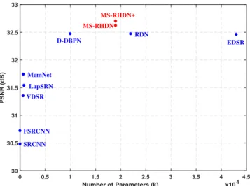
FIGURE 8.Comparison of our method and the state-of-the-art models on Set5 (×4) with respect to PSNR and the number of parameters.
of parameters, we design another 8 network structures with 480
approximate parameters by varying the numbers of MS-RHDB and SDB.
Hierarchical dense module (HDM).To demonstrate the effect of our HDM, we add in different configurations with LDG, ISC, or/and CSC. In table 3, when LDG, ISC, and CSC 485
are absent, the PSNR value on Set5 is relatively low. The positive effect of LDG is demonstrated by the performance improvement from structure 1 to 3. Similarly, ISC and CSC are significant for producing high-quality images. The perfor-mance increases with LDG, ISC, or CSC, and we can obtain 490
improvements by using all of them. After adding HDMs, the performance increases to 31.93 dB compared to the structure 1 with 31.50 dB. This demonstrates the efficiency of our HDM in extracting informative features.
Multi-scale block. Finally, we show the effect of the 495
multi-scale block based on the observations from Table 3.
When MSBs are added, the PSNR value increases from 31.93 dB in structure 6 to 32.05 dB in structure 9. Comparisons between structure 1 and 2 or structure 4 and 7 demonstrate
the effectiveness of the MSB as well. The performance 500
improvements obtained by the MSB indicate that the multi-scale features have played an important part in generating SR images.
In Fig.7, we further visualize the training process of these nine structures on the PSNR of Set5 (×4). We can observe 505 that the curves are consistent with our analyses, and the LDG, ISC, CSC, and MSB can further improve the performance. These quantitative and visual analyses show the superiority and effectiveness of our proposed LDG, ISC, CSC, and MSB
elements. 510
Fig.8 shows comparisons of PSNR versus the number of parameters of our method and the compared methods. We can observe that our MS-RHDN and MS-RHDN+ have only half number of parameters of EDSR [7] and also fewer parameters
than RDN [31]. They also achieve better performance. It 515
demonstrates that our model has a more effective structure and a better trade-off between performance and model size.
VI. CONCLUSIONS
In this paper, we propose a novel multi-scale residual
hierarchical dense network for high-quality image super- 520
resolution. Our model aims at fully utilizing features in LR images. Specifically, the residual hierarchical dense struc-ture is used for adaptively extracting multi-level feastruc-tures. Meanwhile, the multi-scale block serves to obtain multi-scale features. Furthermore, residual learning mechanism is used 525 to stabilize the training of our model, and to pay attention to more informative features. Extensive experiments on bench-mark datasets illustrate the effectiveness of our MS-RHDN in image super-resolution.
REFERENCES 530
[1] C. Dong, C. C. Loy, K. He, and X. Tang, “Image super-resolution using deep convolutional networks,” IEEE Transactions on Pattern Analysis and Machine Intelligence, vol. 38, no. 2, pp. 295–307, 2016.
[2] J. Kim, J. K. Lee, and K. M. Lee, “Accurate image super-resolution using very deep convolutional networks,” in 2016 IEEE Conference on 535
Computer Vision and Pattern Recognition (CVPR), Jun. 2016, pp. 1646– 1654.
[3] C. Dong, C. C. Loy, K. He, and X. Tang, “Image super-resolution using deep convolutional networks,” IEEE Transactions on Pattern Analysis and Machine Intelligence, vol. 38, no. 2, pp. 295–307, Feb. 2016. 540
[4] W. Lai, J. Huang, N. Ahuja, and M. Yang, “Deep laplacian pyramid networks for fast and accurate super-resolution,” in 2017 IEEE Conference on Computer Vision and Pattern Recognition (CVPR), Jul. 2017, pp. 5835–5843.
[5] W. Lai, J. Huang, N. Ahuja, and M. Yang, “Fast and accurate image super- 545
resolution with deep Laplacian pyramid networks,” IEEE Transactions on Pattern Analysis and Machine Intelligence, pp. 1–14, Aug. 2018. [6] K. He, X. Zhang, S. Ren, and J. Sun, “Deep residual learning for image
recognition,” in 2016 IEEE Conference on Computer Vision and Pattern Recognition (CVPR), Jun. 2016, pp. 770–778. 550
[7] B. Lim, S. Son, H. Kim, S. Nah, and K. M. Lee, “Enhanced deep residual networks for single image super-resolution,” in 2017 IEEE Conference on Computer Vision and Pattern Recognition Workshops (CVPRW), Jul. 2017, pp. 1132–1140.
[8] R. Timofte, E. Agustsson, L. V. Gool, M. Yang, L. Zhang, B. Lim, S. Son, 555
C. Dong, L. Lin, Y. Qiao, C. C. Loy, W. Bae, J. Yoo, Y. Han, J. C. Ye, J. Choi, M. Kim, Y. Fan, J. Yu, W. Han, D. Liu, H. Yu, Z. Wang, H. Shi, X. Wang, T. S. Huang, Y. Chen, K. Zhang, W. Zuo, Z. Tang, L. Luo, S. Li, M. Fu, L. Cao, W. Heng, G. Bui, T. Le, Y. Duan, D. Tao, R. Wang, X. Lin,
560
J. Pang, J. Xu, Y. Zhao, X. Xu, J. Pan, D. Sun, Y. Zhang, X. Song, Y. Dai, X. Qin, X. Huynh, T. Guo, H. S. Mousavi, T. H. Vu, V. Monga, C. Cruz, K. Egiazarian, V. Katkovnik, R. Mehta, A. K. Jain, A. Agarwalla, C. V. S. Praveen, R. Zhou, H. Wen, C. Zhu, Z. Xia, Z. Wang, and Q. Guo, “Ntire 2017 challenge on single image super-resolution: Methods and results,”
565
in 2017 IEEE Conference on Computer Vision and Pattern Recognition Workshops (CVPRW), Jul. 2017, pp. 1110–1121.
[9] Y. Tai, J. Yang, and X. Liu, “Image super-resolution via deep recursive residual network,” in 2017 IEEE Conference on Computer Vision and Pattern Recognition (CVPR), Jul. 2017, pp. 2790–2798.
570
[10] H. Hou and H. Andrews, “Cubic splines for image interpolation and digital filtering,” IEEE Transactions on Acoustics, Speech, and Signal Processing, vol. 26, no. 6, pp. 508–517, Dec. 1978.
[11] X. Li and M. T. Orchard, “New edge-directed interpolation,” IEEE Trans-actions on Image Processing, vol. 10, no. 10, pp. 1521–1527, Oct. 2001.
575
[12] L. Zhang and X. Wu, “An edge-guided image interpolation algorithm via directional filtering and data fusion,” IEEE Transactions on Image Processing, vol. 15, no. 8, pp. 2226–2238, Aug. 2006.
[13] M. Li and T. Q. Nguyen, “Markov random field model-based edge-directed image interpolation,” IEEE Transactions on Image Processing, vol. 17,
580
no. 7, pp. 1121–1128, Jul. 2008.
[14] M. Irani and S. Peleg, “Improving resolution by image registration,” CVGIP: Graphical Models and Image Processing, vol. 53, no. 3, pp. 231– 239, 1991.
[15] S. Baker and T. Kanade, “Limits on super-resolution and how to break
585
them,” IEEE Transactions on Pattern Analysis and Machine Intelligence, vol. 24, no. 9, pp. 1167–1183, Sep. 2002.
[16] Z. Lin and H.-Y. Shum, “Fundamental limits of reconstruction-based superresolution algorithms under local translation,” IEEE Transactions on Pattern Analysis and Machine Intelligence, vol. 26, no. 1, pp. 83–97, Jan.
590
2004.
[17] W. T. Freeman and E. C. Pasztor, “Learning low-level vision,” in Proceed-ings of the Seventh IEEE International Conference on Computer Vision, vol. 2, Sep. 1999, pp. 1182–1189.
[18] H. Chang, D.-Y. Yeung, and Y. Xiong, “Super-resolution through neighbor
595
embedding,” in 2004 IEEE Computer Society Conference on Computer Vision and Pattern Recognition (CVPR), vol. 1, Jun. 2004, pp. 1–1. [19] S. T. Roweis and L. K. Saul, “Nonlinear dimensionality reduction by
locally linear embedding,” Science, vol. 290, no. 5500, pp. 2323–2326, 2000.
600
[20] R. Timofte, V. De, and L. V. Gool, “Anchored neighborhood regression for fast example-based super-resolution,” in 2013 IEEE International Confer-ence on Computer Vision (ICCV), Dec. 2013, pp. 1920–1927.
[21] R. Timofte, V. De Smet, and L. Van Gool, “A+: Adjusted anchored neighborhood regression for fast super-resolution,” in Asian Conference
605
on Computer Vision (ACCV), 2014, pp. 111–126.
[22] J. Huang and W. Siu, “Learning hierarchical decision trees for single-image super-resolution,” IEEE Transactions on Circuits and Systems for Video Technology, vol. 27, no. 5, pp. 937–950, May. 2017.
[23] J. Huang and W. Siu, “Practical application of random forests for
super-610
resolution imaging,” in 2015 IEEE International Symposium on Circuits and Systems (ISCAS), May. 2015, pp. 2161–2164.
[24] J. Huang, W. Siu, and T. Liu, “Fast image interpolation via random forests,” IEEE Transactions on Image Processing, vol. 24, no. 10, pp. 3232–3245, Oct. 2015.
615
[25] S. Schulter, C. Leistner, and H. Bischof, “Fast and accurate image upscal-ing with super-resolution forests,” in 2015 IEEE Conference on Computer Vision and Pattern Recognition (CVPR), Jun. 2015, pp. 3791–3799. [26] D. Xiong, Q. Gui, W. Hou, and M. Ding, “Gradient boosting for single
image super-resolution,” Information Sciences, vol. 454, pp. 328–343,
620
2018.
[27] W. Shi, J. Caballero, F. Huszà ˛ar, J. Totz, A. P. Aitken, R. Bishop, D. Rueckert, and Z. Wang, “Real-time single image and video super-resolution using an efficient sub-pixel convolutional neural network,” in 2016 IEEE Conference on Computer Vision and Pattern Recognition
625
(CVPR), Jun. 2016, pp. 1874–1883.
[28] K. Zhang, W. Zuo, and L. Zhang, “Learning a single convolutional super-resolution network for multiple degradations,” in 2018 IEEE Conference on Computer Vision and Pattern Recognition (CVPR), Jun. 2018, pp. 3262–3271.
630
[29] A. Shocher, N. Cohen, and M. Irani, “Zero-shot super-resolution using deep internal learning,” in 2018 IEEE Conference on Computer Vision and Pattern Recognition (CVPR), Jun. 2018, pp. 3118–3126.
[30] M. Haris, G. Shakhnarovich, and N. Ukita, “Deep back-projection net-works for super-resolution,” in 2018 IEEE Conference on Computer 635
Vision and Pattern Recognition (CVPR), Jun. 2018, pp. 1664–1673. [31] Y. Zhang, Y. Tian, Y. Kong, B. Zhong, and Y. Fu, “Residual dense network
for image super-resolution,” in 2018 IEEE Conference on Computer Vision and Pattern Recognition (CVPR), Jun. 2018, pp. 2472–2481.
[32] Y. Zhang, K. Li, K. Li, B. Zhong, and Y. Fu, “Residual non-local attention 640
networks for image restoration,” in International Conference on Learning Representations (ICLR), 2019.
[33] C. Ledig, L. Theis, F. Huszà ˛ar, J. Caballero, A. Cunningham, A. Acosta, A. Aitken, A. Tejani, J. Totz, Z. Wang, and W. Shi, “Photo-realistic single image super-resolution using a generative adversarial network,” in 2017 645
IEEE Conference on Computer Vision and Pattern Recognition (CVPR), Jul. 2017, pp. 105–114.
[34] X. Wang, K. Yu, S. Wu, J. Gu, Y. Liu, C. Dong, Y. Qiao, and C. C. Loy, “Esrgan: Enhanced super-resolution generative adversarial networks,” in The European Conference on Computer Vision Workshops (ECCVW), 650
Sep. 2018.
[35] A. Jolicoeur-Martineau, “The relativistic discriminator: a key element missing from standard GAN,” arXiv preprint arXiv:1807.00734, 2018. [36] C. Szegedy, S. Ioffe, V. Vanhoucke, and A. A. Alemi, “Inception-v4,
Inception-Resnet and the impact of residual connections on learning,” in 655
Thirty-First AAAI Conference on Artificial Intelligence, 2017. [37] J. Johnson, A. Alahi, and L. Fei-Fei, “Perceptual losses for real-time style
transfer and super-resolution,” in The European conference on computer vision (ECCV), 2016, pp. 694–711.
[38] K. Simonyan and A. Zisserman, “Very deep convolutional networks for 660
large-scale image recognition,” arXiv preprint arXiv:1409.1556, 2014. [39] R. Mechrez, I. Talmi, F. Shama, and L. Zelnik-Manor,
“Maintain-ing natural image statistics with the contextual loss,” arXiv preprint arXiv:1803.04626, pp. 1–16, 2018.
[40] J. Kim and J. Lee, “Deep residual network with enhanced upscaling 665
module for super-resolution,” in 2018 IEEE/CVF Conference on Computer Vision and Pattern Recognition Workshops (CVPRW), June 2018, pp. 913–9138.
[41] G. Huang, Z. Liu, L. v. d. Maaten, and K. Q. Weinberger, “Densely con-nected convolutional networks,” in 2017 IEEE Conference on Computer 670
Vision and Pattern Recognition (CVPR), Jul. 2017, pp. 2261–2269. [42] Y. Tai, J. Yang, X. Liu, and C. Xu, “Memnet: A persistent memory
network for image restoration,” in 2017 IEEE International Conference on Computer Vision (ICCV), Oct. 2017, pp. 4549–4557.
[43] L.-C. Chen, G. Papandreou, F. Schroff, and H. Adam, “Rethinking 675
atrous convolution for semantic image segmentation,” arXiv preprint arXiv:1706.05587, 2017.
[44] Z. Tang, S. Li, L. Luo, M. Fu, H. Peng, and Q. Zhou, “Image super-resolution via simplified dense network with non-degenerate layers,” IEEE
Access, pp. 1–1, 2019. 680
[45] Z. Wang, D. Liu, J. Yang, W. Han, and T. Huang, “Deep networks for image super-resolution with sparse prior,” in 2015 IEEE International Conference on Computer Vision (ICCV), Dec. 2015, pp. 370–378. [46] T. Peleg and M. Elad, “A statistical prediction model based on sparse
representations for single image super-resolution,” IEEE Transactions on 685
Image Processing, vol. 23, no. 6, pp. 2569–2582, Jun. 2014.
[47] K. Zhang, W. Zuo, S. Gu, and L. Zhang, “Learning deep cnn denoiser prior for image restoration,” in 2017 IEEE Conference on Computer Vision and Pattern Recognition (CVPR), Jul. 2017, pp. 2808–2817.
[48] M. Bevilacqua, A. Roumy, C. Guillemot, and M.-L. Alberi Morel, “Low- 690
complexity single-image super-resolution based on nonnegative neighbor embedding,” in Proceedings of the British Machine Vision Conference. BMVA Press, 2012, pp. 135.1–135.10.
[49] R. Zeyde, M. Elad, and M. Protter, “On single image scale-up using sparse-representations,” in Proceedings of the 7th International Conference on 695
Curves and Surfaces, 2012, pp. 711–730.
[50] D. Martin, C. Fowlkes, D. Tal, and J. Malik, “A database of human segmented natural images and its application to evaluating segmentation algorithms and measuring ecological statistics,” in 2001 IEEE Interna-tional Conference on Computer Vision (ICCV), vol. 2, Jul. 2001, pp. 416– 700
423.
[51] J. Huang, A. Singh, and N. Ahuja, “Single image super-resolution from transformed self-exemplars,” in 2015 IEEE Conference on Computer Vision and Pattern Recognition (CVPR), Jun. 2015, pp. 5197–5206.
[52] Y. Matsui, K. Ito, Y. Aramaki, A. Fujimoto, T. Ogawa, T. Yamasaki,
705
and K. Aizawa, “Sketch-based manga retrieval using manga109 dataset,” Multimedia Tools and Applications, vol. 76, no. 20, pp. 21 811–21 838, 2017.
[53] D. P. Kingma and J. Ba, “Adam: A method for stochastic optimization,” arXiv preprint arXiv:1412.6980, 2014.
710
[54] A. Paszke, S. Gross, S. Chintala, G. Chanan, E. Yang, Z. DeVito, Z. Lin, A. Desmaison, L. Antiga, and A. Lerer, “Automatic differentiation in pytorch,” 2017.
[55] R. Timofte, R. Rothe, and L. V. Gool, “Seven ways to improve example-based single image super resolution,” in 2016 IEEE Conference on
Com-715