Code Transformations for Energy-Efficient
Device Management
Taliver Heath, Eduardo Pinheiro, Jerry Hom, Ulrich Kremer, and Ricardo Bianchini
Department of Computer Science, Rutgers University
taliver,edpin,jhom,uli,ricardob
@cs.rutgers.edu
Abstract
Energy conservation without performance degradation is an important goal for
battery-operated computers, such as laptops and hand-held assistants. In this paper we study
application-supported device management for optimizing energy and performance. In par-ticular, we consider application transformations that increase device idle times and inform the operating system about the length of each upcoming period of idleness. We use modeling and experimentation to assess the potential energy and performance benefits of this type of application support for a laptop disk. Furthermore, we propose and evaluate a compiler frame-work for performing the transformations automatically. Our main modeling results show that the transformations are potentially beneficial. However, our experimental results with six real laptop applications demonstrate that unless applications are transformed, they cannot accrue any of the predicted benefits. In addition, they show that our compiler can produce almost the same performance and energy results as hand-modifying applications. Overall, we find that the transformations can reduce disk energy consumption from 55% to 89% with a degradation in performance of at most 8%.
1
Introduction
Recent years have seen a substantial increase in the amount of research on battery-operated com-puters. The main goal of this research is to develop hardware and software that can improve energy efficiency and, as a result, lengthen battery life. The most common approach to achieving energy efficiency is to put idle resources or entire devices in low-power states until they have to be ac-cessed again. The transition to a lower power state usually occurs after a period of inactivity (an
inactivity threshold), and the transition back to active state usually occurs on demand. The
tran-sitions to and from low-power states incur time and energy penalties. Nevertheless, this strategy works well when there is enough idle time to justify incurring such costs.
Previous studies of device control for energy efficiency have shown that some workloads do exhibit relatively long idle times. However, these studies were limited to interactive applications (or their traces), slow microprocessors, or both. Recent advances in fast, low-power microproces-sors and their use in battery-operated computers are increasing the number of potential applications for these computers. For instance, nowadays laptop users frequently run non-interactive applica-tions, such as movie playing, decompression, and encryption. For most of these applicaapplica-tions, fast processors reduce device idle times, which in turn reduce the potential for energy savings. Fur-thermore, incurring re-activation delays in the critical path of the microprocessor now represents a more significant overhead (in processor cycles), as re-activation times are not keeping pace with microprocessor speed improvements.
Thus, to maximize our ability to conserve energy without degrading performance under these new circumstances, we need ways to increase device idle times, eliminate inactivity thresholds, and start re-activations in advance of device use. Device idle times can be increased in several ways and at many levels, such as by energy-aware scheduling or prefetching in the operating system, by performing loop transformations during compilation, etc. The set of possibilities for achieving the other two goals is more limited. In fact, those goals can only be achieved with fairly accurate predictions of future application behavior, which can be produced with programmer
or compiler involvement. For these reasons, we advocate that programmers or compilers, i.e. applications, should be directly involved in device control in single-user, battery-operated systems such as laptops.
To demonstrate the benefits of this involvement, in this paper we evaluate the effect of trans-forming explicit I/O-based applications to increase their device idle times. These transformations may be performed by a sophisticated compiler, but can also be implemented by the programmer after a sample profiling run of the application. For greater benefits, the transformations must in-volve an approximate notion of the original and target device idle times. Thus, we also evaluate the effect of having the application inform the duration of each device idle period (hereafter re-ferred to as a CPU run-length, or simply run-length, the time during which the CPU is busy and the device is idle) to the operating system. With this information, the operating system can apply more effective device control policies. (For simplicity, we focus on the common laptop or hand-held scenario in which only one application is ready to run at a time; other applications, such as editors or Web browsers, are usually blocked waiting for user input.) In particular, we study two kernel-level policies, direct deactivation and pre-activation, that rely on run-length information to optimize energy and performance. Direct deactivation eliminates inactivity thresholds, taking the device directly to the best low-power state for a certain run-length, whereas pre-activation removes the device re-activation from the critical computation path.
We develop simple analytical models that describe the isolated and combined energy and per-formance benefits of program transformations and these energy management policies. The models allow a quick assessment of these benefits, as a function of device and application characteristics such as the overhead of device re-activation, and the distribution of run-lengths.
The models are general and apply to any application and device with more than one power state. As a concrete example, we apply them in the control of a laptop disk. Disks are responsible for a significant fraction of the energy consumed by laptops. Li et al. [13] and Douglis et al. [4], for example, report fractions of 20 and 30%. As a result, several techniques have been proposed
for conserving laptop disk energy, e.g. [3, 9, 21, 14, 19].
Interestingly, our experiments with the laptop disk indicate that our initial models were not accurate. The reason is that the disk does not behave exactly as described in the manufacturer’s manuals. As a result, we develop behavior-adjustment models to extend the initial models.
The execution of several applications on our laptop provides the run-length information we plug into the models. Unfortunately, our experiments show that several common applications do not exhibit long enough run-lengths to allow for energy savings. To evaluate the potential of application transformations and application/operating system interaction, we manually transform applications, implement the policies in the Linux kernel, and collect experimental energy and per-formance results. These results show that our adjusted models can accurately predict disk energy consumption and CPU time. Furthermore, the results demonstrate that the transformed applica-tions can conserve a significant amount of disk energy without incurring substantial performance degradation. Compared to the unmodified applications, the transformed applications can achieve disk energy reductions ranging from 55% to 89% with a performance degradation of at most 8%.
Encouraged by these results, we implemented a prototype compiler based on the SUIF2 com-piler infrastructure that automates the manual code transformations and performs run-time profiling to determine run-lengths. Our preliminary results with the compiler infrastructure are as good as those with hand-modified applications.
In summary, we make the following contributions:
We propose transformations to explicit I/O-based applications that increase their CPU run-lengths (and consequently their device idle times). Another transformation informs the op-erating system about the upcoming run-lengths.
We develop analytical models to evaluate our approach to application-supported device man-agement. In this paper, we chose to apply our models to a laptop disk. For this disk, we show that simple and intuitive models are not accurate. With adjusted models, we assess
the behavior of any application. Unfortunately, the adjusted models are neither simple nor intuitive.
We implement and experimentally evaluate our transformations for real applications and a real laptop disk, as they are applied by the programmer or with compiler support. We also consider the effect of operating system-directed prefetching.
The remainder of this paper is organized as follows. The next section discusses the related work. Section 3 details the different policies we consider and presents models for them. Section 4 describes the disk, the application workload, the application transformations, and the compiler framework we propose. The section also presents the results of our analyses and experiments. Finally, section 5 summarizes the conclusions we draw from this research.
2
Related Work
Application support for device control. There have been several proposals for giving applications
greater control of power states [5, 17, 15, 18, 2, 10]. Carla Ellis [5] articulated the benefits of involving applications in energy management, but did not study specific techniques. Lu et al. [17] suggested an architecture for dynamic energy management that encompassed application control of devices, but did not evaluate this aspect of the architecture. In a more recent paper, Lu et al. [15] studied the benefit of allowing applications to specify their device requirements with a single operating system call. Weissel et al. [21] allowed applications to inform the operating system when disk requests are deferrable or even cancelable. Microsoft’s OnNow project [18] suggests that applications should be more deeply involved, controlling all power state transitions. Flinn and Satyanarayanan [7] first demonstrated the benefits of application adaptation.
Our work differs from these approaches in that we propose a different form of application support: one in which the application is transformed to increase its run-lengths and to inform the operating system about each upcoming run-length, after a device access. This strategy
al-lows us to handle short-run-length and irregular applications. Our approach also simplifies pro-gramming/compiler construction (with respect to OnNow) without losing any energy conservation opportunities.
Delaluz et al. [2] and Hom and Kremer [10] are developing compiler infrastructure for similar approaches to application support. Delaluz et al. transform array-based benchmarks to cluster array variables and conserve DRAM energy, whereas Hom and Kremer transform such benchmarks to cluster page faults and conserve wireless interface energy. Both groups implement their energy management policies in the compiler and use simulation to evaluate their transformations.
In our approach, the compiler or programmer is responsible for performing transformations to increase the possible energy savings, but the actual management policies are implemented in the operating system for three reasons: (1) the kernel is traditionally responsible for managing all devices; (2) the kernel can reconcile information from multiple applications; and (3) the kernel can actually reduce any inaccuracies in the run-length information provided by the application, accord-ing to previously observed run-lengths or current system conditions; the compiler does not have access to that information. Nevertheless, our work is complementary to theirs in that we
exper-imentally study a different form of application transformation under several energy conservation
policies.
Analytical Modeling. We are aware of only a few analytical studies of energy management
strate-gies. Greenawalt [8] developed a statistical model of the interval between disk accesses using a Poisson distribution. Fan et al. [6] developed a statistical model of the interval between DRAM accesses using an exponential distribution. In both cases, modeling the arrival of accesses as a memoryless distribution does not seem appropriate, as suggested by the success of history-based policies [3, 2].
Furthermore, our combination of modeling and experimentation is important in that the models determine the region in the parameter space where application support is most effective, whereas the experiments determine the region where applications actually lie.
Direct Deactivation and Pre-activation. As far as we know, only recently have
application-supported policies for device deactivation and pre-activation been proposed [2, 10]. Other works, such as [4], simulate idealized policies that are equivalent to having perfect knowledge of the future and applying both direct deactivation and pre-activation. Rather than simulate, we implement and experimentally evaluate direct deactivation and pre-activation.
Conserving Disk Energy. Disks have been a frequent focus of energy conservation research, e.g.
[22, 13, 4, 3, 9, 17, 11, 8, 16, 21, 14]. The vast majority of the previous work has been on history-based, adaptive-threshold policies, such as the one used in IBM disks. Because our application-supported policies can use information about the future, they can conserve more energy and avoid performance degradation more effectively than history-based strategies. Furthermore, we focus on non-interactive applications and application-supported disk control.
3
Models
In this section, we develop simple and intuitive models of five device control policies: Energy-Oblivious (EO), Fixed-Thresholds (FT), Direct Deactivation (DD), Pre-Activation (PA), and Com-bined DD + PA (CO). The models predict device energy consumption and CPU performance, based on parameters such as power consumption at each device state and application run-lengths.
For the purpose of terminology, we define the power states to start at number 0, the active state, in which the device is being actively used and consumes the most power. The next state, state 1, consumes less power than state 0. In state 1, there is no energy or performance overhead to use the device. Each of the next (larger or deeper) states consumes less power than the previous state, but involves more energy and performance overhead to re-activate. Re-activations bring the device back to state 1.
Before presenting the models, we state our assumptions: (1) We assume that run-lengths are exact. This assumption means that we are investigating the upper-bound on the benefits of the
policies that exploit DD and PA. In practice, we expect that run-lengths can be approximated with good enough accuracy to accrue most of these benefits; (2) We assume that the application calls to the operating system have negligible time and energy overheads. Our experiments show that these overheads are indeed insignificant in practice. For example, the implementation of the DD policy for disk control takes on the order of tens of microseconds to execute on a fast processor, compared to run-lengths on the order of milliseconds; and (3) We assume that run-lengths are delimited by device operations that occur in the critical path of the CPU processing (e.g. blocking disk reads that miss in the file system buffer cache). The models can be extended to consider non-blocking accesses, but this is beyond the scope of this paper.
3.1
Modeling the Energy-Oblivious Policy
The EO control policy keeps the device at its highest idle power state, so that an access can be immediately started at any time. Thus, this policy promotes performance, regardless of energy considerations.
We model a device under the EO policy to use energy per run-length (
) that is the product of
the run-length ( ) and the power consumption when the device is in state 1 ( ), i.e. .
The CPU time per run-length under the EO policy (
) is simply the run-length, i.e.
.
3.2
Modeling the Fixed-Thresholds Policy
The FT control policy recognizes the need to conserve energy in battery-operated computers. It determines that a device should be sent to the consecutive lower power states after fixed periods of inactivity. We refer to these periods as inactivity thresholds. For example, the device could be put in state 2 from state 1 after an inactivity period of 4 seconds (the inactivity threshold for state 1), and later be sent to state 3 after another 8 seconds (the threshold for state 2), and so on. Thus, after 12 seconds the device would have gone from state 1 to state 3.
We define the energy consumed by the device under FT per run-length ( ) as the sum of
three components: the energy spent going from state 1 to the state before the final state , the
energy spent at state , and the energy necessary to re-activate the device starting at state . Thus,
. In this equation,
represents the power consumed at state ,
is the time spent at state
(equal to the inactivity threshold for this state),
is the energy consumed when going from
state to
!
, and " is the re-activation energy from state
to state 1. The final state is
the lowest power state that can be reached within the run-length, i.e. the largest state such that
$# .
The CPU time per run-length (
) is then the run-length plus the time to re-activate from state
( ), i.e. . Note that = 0 and
= 0, because in state 1 the device is ready to be used. In addition,
the time consumed by the transition from state to a lower power state&%,
'"(
, does not appear
in the time equations because it is not in the critical path of the CPU.
FT can be implemented by the operating system (according to the ACPI standard [1]) or by the device itself. These implementation differences are of no consequence to our model. In fact, since FT conserves energy in a well-understood fashion, we use it as a basis for comparison.
3.3
Modeling the Direct Deactivation Policy
FT is based on the assumption that if the device is not accessed for a certain amount of time, it is unlikely to be accessed for a while longer. If we knew the run-lengths a priori, we could save even more energy by simply putting the device in the desired state right away. This is the idea behind the DD control policy, i.e. use application-level knowledge to maximize the energy savings.
We model the device energy consumed per run-length under DD (
'
) as the energy consumed to get to the low power state, plus the energy consumed at that state, and the energy required to
re-activate the device, i.e. ( " .
Note that we differentiate between states and %, as FT and DD do not necessarily reach
the same final state for the same run-length. In fact, % is defined to be the lowest power state
for which going to the next state would consume more energy, i.e. the largest state such that
( ( ( " # ( ( ( " .
The CPU time per run-length for DD (
'
) is then similar to that for FT:
' ( ".
3.4
Modeling the Pre-Activation Policy
In both FT and DD, the time to bring the device back from a low-power state to state 1 is exposed to applications, as the transition is triggered by the device access itself. However, with run-length information from the application, we can hide the re-activation overhead behind useful computa-tion. This is the idea behind PA, i.e. to allow energy savings (through FT or DD) while avoiding performance degradation. For maximum energy savings, the pre-activated device should reach state 1 “just before” it will be accessed. The specific version of PA that we model uses FT to save energy. PA should achieve the same performance as EO, but with a lower energy consumption.
We model the device energy consumed per run-length under PA (
) as (( ' (( (( (( (( ".
Again, we highlight that the final low-power state %% need not be the same as for FT and DD for
the same run-length, because re-activation occurs earlier with device pre-activation. %% is defined
as the highest power state such that
(( (( .
The CPU time per run-length under this policy (
) is
.
3.5
Modeling the Combined Policy
We can achieve the greatest energy savings without performance degradation by combining PA and DD. This is the idea behind the CO policy.
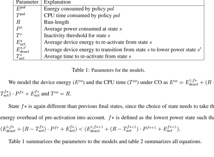
Parameter Explanation
Energy consumed by policy
CPU time consumed by policy
Run-length
Average power consumed at state
Inactivity threshold for state
Average device energy to re-activate from state
'(
" Average device energy to transition from state
to lower power state&%
Average time to re-activate from state
Table 1: Parameters for the models.
We model the device energy (
) and the CPU time (
) under CO as and .
State is again different than previous final states, since the choice of state needs to take the
energy overhead of pre-activation into account. is defined as the lowest power state such that
# " .
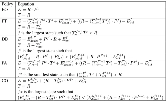
Table 1 summarizes the parameters to the models and table 2 summarizes all equations.
3.6
Modeling Whole Applications
So far, we presented models that compute energy and time based on a single run-length. These models could be applied directly to determine the energy and time consumed by an application, if we could somehow find a run-length that represented all run-lengths of the application. This is easy to do for an application in which all run-lengths are of the same size. Unfortunately, few applications are this well-behaved. Another option would be to use the average run-length. However, the average run-length is not a good choice for two reasons: (1) applications may exhibit widely varying run-lengths, making average calculations meaningless; and (2) the models are non-linear, so modeling energy and time based on the average run-length would not be accurate, even if the average could be meaningfully computed.
Instead of using the average run-length, we model applications by separating run-lengths into ranges or groups for which the models are linear, i.e. groups are associated with power states. For
Policy Equation EO FT ' "
is the largest state such that
# DD ( ( ( (
% is the largest state such that
( ( ( # ( " ( ( PA (( ' " (( (( " (( ((
%% is the smallest state such that
(( (( CO
is the largest state such that
" # "
Table 2:Energy and time equations for all policies.
instance, under FT, we define the groups according to the inactivity thresholds, i.e. group 1 is the
set of run-lengths such that
#
, group 2 is the set of run-lengths such that
#
,
and so on. This grouping scheme allows us to work with the run-length exactly in the middle of each range, as the average run-length for the group. However, using these run-lengths we would not know whether we were underestimating or overestimating energy and time.
Instead of doing that, we find it more interesting to bound the energy and time consumed by applications below and above, using the minimum and maximum values in the groups, respectively. Besides, focusing on upper and lower bounds obviates the need to determine the distribution of run-lengths, which has been shown a complex proposition [6]. For a whole application, the upper and lower bounds on energy and time depend solely on the fraction of the run-lengths that fall within each group. More specifically, the overall potential of each policy is lower bounded by the sum of the minimums and upper bounded by the sum of the maximums. For instance, under FT, if all run-lengths for an application are in group 2, the minimum energy consumption occurs when all
Application transformations that lengthen run-lengths have the potential to increase energy savings. In terms of our groups, lengthening run-lengths increases the fraction of run-lengths in larger numbered groups, with a corresponding decrease in the fraction of run-lengths in smaller numbered groups.
4
Evaluation for a Laptop Disk
The models above are not specific to any application or device. In fact, they can easily be applied to a variety of applications (such as communication or disk-bound applications) and devices (such as network interfaces or disks). The key is that applications and devices should have well-defined run-lengths and power states, respectively.
As an example device, this section applies our models in the control of a Fujitsu MHK2060AT laptop disk, which can be found in a number of commercial laptops. The section also details the application transformations and the implementations of the management policies for the disk. Our study of this disk is representative of other laptop disks.
The section proceeds as follows. First, we adjust the models for our disk and instantiate their parameters. Next, we measure the run-lengths of several laptop-style applications on a 667 MHz Pentium III-based system to find the policies’ potential in practice. After that, we discuss the ben-efits achievable by these applications. This leads us to the specific transformations and compiler framework we propose. Last, to corroborate the models, we run both original and modified ap-plications with and without operating system prefetching, and measure the resulting energy and performance gains.
4.1
The Fujitsu Disk
The Fujitsu disk is a 6-Gbyte, 4200-rpm drive with ATA-5 interface. According to its manual, it only implements four power states:
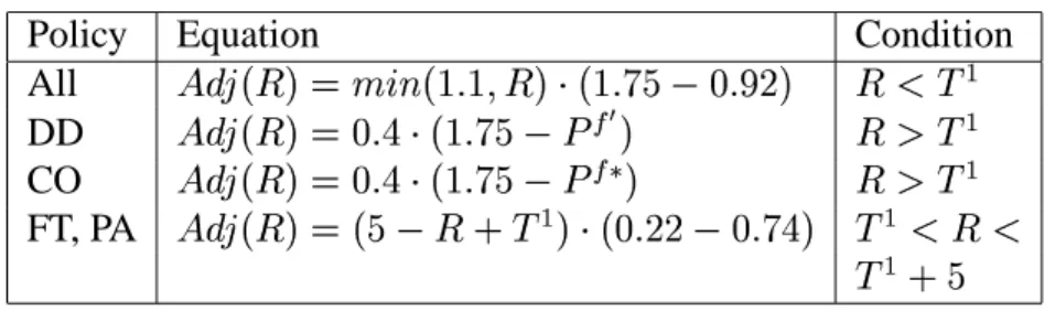
Policy Equation Condition All # DD ( CO FT, PA # #
Table 3: Energy adjustment models for all policies.
0. Active – the disk is performing a read or a write access.
1. Idle – all electronic components are powered on and the storage medium is ready to be accessed. This state is entered after the execution of a read or write. This state consumes 0.92 W.
2. Standby – the spindle motor is powered off, but the disk interface can still accept commands. This state consumes 0.22 W.
3. Sleep – the interface is inactive and the disk requires a software reset to be re-activated. This state consumes 0.08 W.
However, our experiments demonstrate that there are two hidden transitional states. The first occurs before a transition from active to idle. Right after the end of an access, the disk moves to the hidden state. There, it consumes 1.75 W for at most 1.1 secs, regardless of policy. The disk also goes into this hidden state for 0.4 secs when we transition to standby or sleep in DD or CO. The second hidden state occurs when we transition from idle (FT and PA) or the first hidden state (DD and CO) to standby or sleep. Before arriving at the final state, the disk consumes 0.74 W at this hidden state for at most 5 secs. (The entire overhead of this hidden state, 5 secs at 0.74 W, is
included in
from idle state in our modeling.) We do not number these extra states. To make
the models more accurate, we extend them to account for the hidden states. The adjustment factors for energy are listed in table 3. No time adjustments are needed.
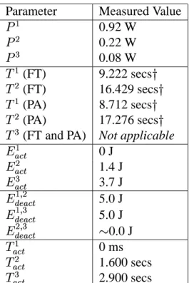
Table 4 lists the measured value for each of the parameters of our models. The measurements
Parameter Measured Value 0.92 W 0.22 W 0.08 W (FT) 9.222 secs (FT) 16.429 secs (PA) 8.712 secs (PA) 17.276 secs
(FT and PA) Not applicable
" 0 J " 1.4 J " 3.7 J 5.0 J 5.0 J 0.0 J " 0 ms " 1.600 secs " 2.900 secs
Table 4: Model parameters and measured values for the Fujitsu disk. Values marked with “
” were picked so that $ $ .
disk should stay at a higher power state only as long as it has consumed the same energy it would have consumed at the next lower power state, i.e.
' .
The rationale for this assumption is similar to the famous competitive argument about renting or buying skis [12].
4.2
Model Predictions
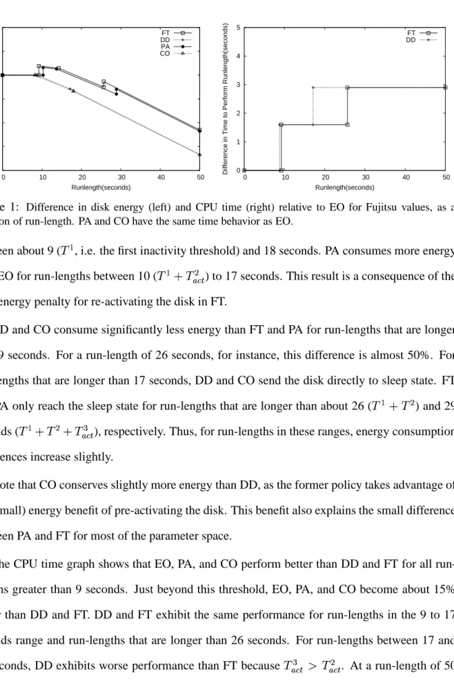
Given the energy and time values of the disk, we can evaluate the policies with our models’ predic-tions. Figure 1 plots the difference in disk energy relative to EO (left) and the difference in CPU time relative to EO (right) for each policy, as a function of run-length. Since PA and CO have the same time behavior as EO, we do not include these policies in the time graph. The figure assumes our adjusted models.
The energy graph shows that FT and PA consume the most energy out of the energy-conscious policies. In fact, FT consumes significantly more energy than even the EO policy for run-lengths
-40 -30 -20 -10 0 10 20 0 10 20 30 40 50
Difference in Energy to Perform Runlength(J)
Runlength(seconds) FT DD PA CO 0 1 2 3 4 5 0 10 20 30 40 50
Difference in Time to Perform Runlength(seconds)
Runlength(seconds)
FT DD
Figure 1: Difference in disk energy (left) and CPU time (right) relative to EO for Fujitsu values, as a
function of run-length. PA and CO have the same time behavior as EO.
between about 9 ( , i.e. the first inactivity threshold) and 18 seconds. PA consumes more energy
than EO for run-lengths between 10 (
) to 17 seconds. This result is a consequence of the
high energy penalty for re-activating the disk in FT.
DD and CO consume significantly less energy than FT and PA for run-lengths that are longer than 9 seconds. For a run-length of 26 seconds, for instance, this difference is almost 50%. For run-lengths that are longer than 17 seconds, DD and CO send the disk directly to sleep state. FT
and PA only reach the sleep state for run-lengths that are longer than about 26 (
) and 29 seconds (
), respectively. Thus, for run-lengths in these ranges, energy consumption
differences increase slightly.
Note that CO conserves slightly more energy than DD, as the former policy takes advantage of the (small) energy benefit of pre-activating the disk. This benefit also explains the small difference between PA and FT for most of the parameter space.
The CPU time graph shows that EO, PA, and CO perform better than DD and FT for all run-lengths greater than 9 seconds. Just beyond this threshold, EO, PA, and CO become about 15% better than DD and FT. DD and FT exhibit the same performance for run-lengths in the 9 to 17 seconds range and run-lengths that are longer than 26 seconds. For run-lengths between 17 and
26 seconds, DD exhibits worse performance than FT because
seconds, the performance difference between the policies is approximately 5%.
4.3
Benefits for Applications
As mentioned in section 3.6, we group run-lengths with respect to power states to model whole
applications. Under FT, for instance, we divide run-lengths into 3 groups: [1,
], [ ,
],
and [ , 49999]. As is apparent in this break down, we use 1 millisecond and 50 seconds as the
shortest and longest possible run-lengths, respectively. (We have found experimentally that only a few run-lengths in our original and modified applications do not fall in this range.)
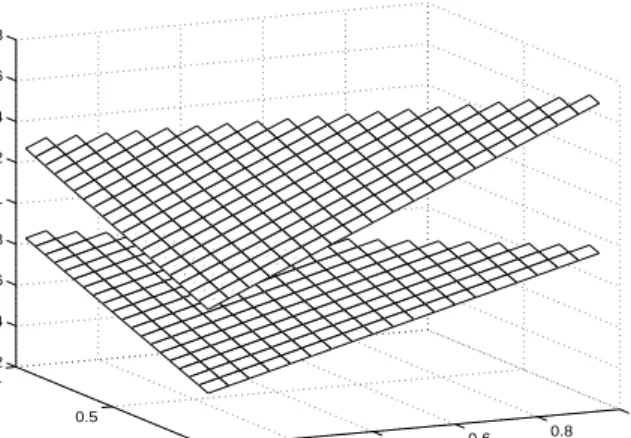
Figure 2 plots the average power (energy/sec) consumed by applications under DD (left) and PA (right), as a function of the percentage of run-lengths that fall within the groups associated with states 1 (idle) and 2 (standby). The run-lengths associated with state 3 (sleep) are the remaining ones. In both graphs, lower (higher) planes represent minimum (maximum) average power. (We will soon explain what the points in the graphs represent.) Recall that CO has roughly the same power behavior as DD, whereas FT has almost the same power behavior as PA. Consequently, we do not present results for CO and FT explicitly.
The graphs show that run-length distributions that are skewed towards long run-lengths can bring average power to a small fraction of that in state 1, regardless of the policy used. Under an extreme scenario in which all run-lengths are in state 3, i.e. coordinates (0,0,*) in the figures, the minimum average power is roughly 29% (DD) and 50% (PA) lower than the power consumption of state 1. Note that the minimum average power corresponds to the energy consumed by run-lengths of 49.999 seconds plus the energy to re-activate 1 millisecond later, divided by 50 seconds. In contrast, the maximum average power is the result of run-lengths of about 17 (DD) or 29 (PA) seconds and re-activating after 1 millisecond.
Another interesting observation is the significant difference between maximum and minimum consumptions, especially when the percentage of run-lengths in state 1 is large. The largest differ-ences occur at coordinates (1,0,*). For DD, these discrepancies represent the difference between
0 0.2 0.4 0.6 0.8 1 0 0.5 1 0.2 0.4 0.6 0.8 1 1.2 1.4 1.6 1.8 State 1 State 2
Average Power for DD
0 0.2 0.4 0.6 0.8 1 0 0.5 1 0.2 0.4 0.6 0.8 1 1.2 1.4 1.6 1.8 State 1 State 2
Average Power for PA
Figure 2: Average power for DD (left) and PA (right), as a function of the percentage of run-lengths in
states 1, 2, and 3. Lower (higher) plane represents min (max) consumption.
0 0.2 0.4 0.6 0.8 1 0 0.2 0.4 0.6 0.8 1 0 0.05 0.1 0.15 0.2 State 1 State 2
Average Overhead for DD
Figure 3: Average % CPU time overheads of DD policy. Lower (higher) plane represents min (max)
overheads.
having all run-lengths in state 1 be 1 millisecond (maximum) or 9 (minimum) seconds. This differ-ence in the distribution of state 1 run-lengths can cause a factor of almost 2 differdiffer-ence in average power.
Finally, the figures confirm that DD achieves lower average power than PA across the whole parameter space. The only exception is when all run-lengths are in state 1, i.e. at coordinates (1,0,*) in the figures; with this distribution, the two policies produce the same average power. Also, note
that at these coordinates the average power is always higher than
, due to the significant energy
Figure 3 illustrates the percentage CPU time overhead under DD. Results for FT are similar to those in the figure, whereas EO, PA, and CO all exhibit no overhead under our modeling
as-sumptions. The figure shows that minimum overheads are low (#
6%) for most of the parameter space, whereas maximum overheads quickly become significant as the fraction of run-lengths cor-responding to states 2 and 3 is increased. Again, we see the importance of the distribution of run-lengths within each group.
Figures 2 and 3 present the absolute behavior of our policies. However, it is also important to determine the benefits of our policies in comparison to more established policies such as FT. DD can achieve significant energy gains with respect to FT for most of the parameter space. Even the minimum gains are substantial in most of the space. Gains are especially high when most of the run-lengths are within the bounds of state 3. Reducing the percentage of these run-lengths decreases the maximum savings slightly when in favor of state 2 run-lengths and more significantly when in favor of state 1 run-lengths.
In terms of CPU time, PA performs at least as well as FT for the whole parameter space, even in the worst-case scenario. The maximum gains can reach 15%, especially when the distribution of run-lengths is tilted towards state 2. Reducing the percentage of these run-lengths in favor of state 3 run-lengths decreases the maximum savings, but not as quickly as increasing the fraction of state 1 run-lengths.
Figure 2 visualizes the potential benefit of our policies for the entire range of run-length dis-tributions. However, we need to determine where applications actually lie. We measured several applications’ run-lengths by instrumenting the operating system kernel (Linux) on a 667 MHz Pen-tium III-based system to compute that information. (We describe the applications and their inputs later.)
The results of these measurements show that all run-lengths fall in state 1 and, thus, prevent
any energy savings. In terms of the figures we just discussed, this means that applications lie in the
run-lengths, moving the applications towards the left side of the graphs. That is the goal of our proposed application transformations , which we describe in detail in the next subsection.
4.4
Application Transformations
As mentioned above, for non-interactive applications to permit energy savings, we need to increase run-lengths. We propose that run-lengths can be easily increased by modifying the applications’ source codes. In particular, the codes should be modified to cluster disk read operations, so that the processor could process a large amount of data in between two clusters of accesses to disk. If the reads are for consecutive parts of the same file, a cluster of reads can be replaced by a single large read.
Intuitively and supported by figure 2, one might think that the best approach would be to increase run-lengths to the extreme by grouping all reads into a single cluster. However, one must realize that increasing run-lengths in this way would correspondingly increase buffer requirements. Given this direct relationship, we propose that applications should be modified to take advantage of as much buffer space as possible, as long as that does not cause unnecessary disk activity, i.e. swapping. Unfortunately, this approach does not work well for all applications. Streaming media applications, such as video playing, should have the additional restriction of preventing human-perceptible delays in the stream. Therefore, a cluster of reads (or a large read) should take no longer than this threshold. Here, we assume a threshold of 300 milliseconds.
To determine the amount of memory that is available, we propose the creation of a system call. The operating system can then decide how much memory is available for the application to consume and inform the application.
The following example illustrates the transformations on a simple (non-streaming) application based on explicit I/O. Assume that the original application looks roughly like this:
i = 1;
while i <= N {
compute on chunk[i]; i = i + 1;
}
After we transform the application to increase its run-length:
// ask OS how much memory can be used available = how_much_memory();
num_chunks = available/sizeof(chunks); i = 1;
while i <= N {
// cluster read operations
for j = i to min(i+num_chunks, N) read chunk[j] of file;
// cluster computation
for j = i to min(i+num_chunks, N) compute on chunk[j];
i = j + 1; }
A streaming application can be transformed similarly, but the number of chunks
of the file to read (num chunks) should be min(available/sizeof(chunks),
(disk bandwidth x 300 millisecs)/sizeof(chunks)). Regardless of the type of application, the overall effect of this transformation is that the run-lengths generated by the
com-putation loop are nownum chunkstimes as long as the original run-lengths.
As a further transformation, the information about the run-lengths can be passed to the oper-ating system to enable the policies we consider. The sample code above can then be changed to include the following system call in between the read and computation loops:
next_R(appl_specific(available,...));
Note that the next run-length has to be provided by the application itself, based on parameters such as the amount of available memory. Nevertheless, for regular applications, such as streaming audio and video, the operating system could predict run-lengths based on past history, instead of being explicitly informed by the programmer or the compiler. However, the approach we advocate is more general; it can handle these applications, as well as applications that exhibit irregularity.
Our image smoothing application, for instance, smooths all images under a certain directory. As the images are fairly small (can be loaded to memory with a single read call) and of different sizes, each run-length has no relationship to previous ones. Thus, it would be impossible for the operating system to predict run-lengths accurately for this application. In contrast, the compiler or the programmer can approximate each run-length based on the image sizes.
4.5
Compiler Framework
Restructuring the code as described in the previous section is a non-trivial task since it requires an understanding of the performance characteristics of the target platform, including its operat-ing system and disk subsystem. This knowledge is needed to allocate buffers of appropriate size (for streaming applications) and to approximate run-lengths. In addition, manual modifications of source code may introduce bugs and are tedious at best. We have developed a compiler framework and runtime environment that takes the original program with file descriptor annotations as input, and performs the discussed transformations automatically, allowing portability across different tar-get systems and disk performance characteristics.
Our current compiler framework is based on the SUIF2 compiler infrastructure [20] and takes
C programs as input. The user may declare a file descriptor to bestreamedornon-streamed
using declarations of the form: FILE *streamed fd and FILE *non-streamed fd. If no
annotation is specified, I/O operations for the file descriptor will not be modified by the compiler. The compiler propagates file descriptor attributes across procedure boundaries, and replaces every original I/O operation of the file descriptor in the program with calls to a corresponding buffered I/O runtime library.
In cases where procedures have file descriptors as formal parameters, different call sites of
the procedure may use streamed and non-streamed actual parameters, making a simple
replacement of the original file I/O operation within the procedure body impossible. Our current prototype compiler introduces an additional parameter for each such formal file descriptor. The
additional parameter keeps track of the attribute of its corresponding file descriptor. Using the attribute parameter, the compiler generates code that guards any file I/O operation of the formal parameter, resulting in the correct I/O operation selection at runtime. We are investigating the benefits of procedure cloning as an alternative strategy.
The current runtime library contains modified versions ofreadandlseek. The library calls
preserve the semantics of the original I/O operations, and in addition: (1) Measure the perfor-mance of the disk through user-transparent runtime profiling; (2) Measure the data consumption rate by the CPU processing of the disk data; (3) Implement buffered I/O through allocation and management of user-level buffers of appropriate sizes; and (4) Notify the operating system about the expected idle times of the disk (run-lengths).
The main goals of the profiling are to estimate future run-lengths and to determine the maximal buffer size that does not violate the performance constraints of a streaming application. The buffer size should be maximal in order to allow the longest possible disk hibernation time between suc-cessive disk accesses. Sizing the buffer involves approximating the disk’s bandwidth. Our profiling subsystem uses the cost of individual reads from the application to produce a first approximation of the bandwidth. This approximation is used to allocate a test buffer that allows the measurement of the runtime costs of larger reads. From these costs, our profiling subsystem can compute the bandwidth of the disk on larger accesses. The final buffer size is set to the measured large read bandwidth (bytes/second) times the performance constraint (seconds). For a disk where reads of
blocks are much faster than individual block reads, the final buffer size will be significantly
larger than the test buffer size. Figure 4 illustrates the general transitions between these profiling phases. Next, we detail the actions in each phase.
First phase. The first phase (phase 1 in figure 4) measures disk access times to satisfy regular
read requests by the application. Accesses satisfied by the file system buffer cache are ignored in order to compute a lower bound of the disk bandwidth. To detect and ignore the cache fetches, the compiler relies on the time difference between a cache hit and a miss. A buffer cache hit
Refill Buffer and/or Service Request from Buffer Buffer Reads After measuring read
on consecutive blocks and setting buffer size After sufficient reads (tunable)
Phase 3
Phase 1
Observation Disk Measurement Block and Cache ReadsPhase 2
Sustained Throughput MeasurementFigure 4: Phase transition diagram for read requests.
is assumed to take several microseconds, whereas a cache miss (and subsequent disk access) is assumed to take milliseconds.
A global counter keeps track of the number of disk reads measured during the initial profiling phase. The number of reads needed to reach a steady-state measurement depends on the amount of data requested by each read operation. Our current implementation takes this number as an input. However, we believe that the profiler can derive this number based on a histogram of read access times. Once a suitable number of reads have been measured, the average disk bandwidth can be computed, which is a lower bound on the disk’s actual bandwidth.
Second phase. In the second phase (phase 2 in figure 4), several calculations from the previous
measurements lead to two crucial values. First is the lower bound estimate mentioned above. This lower bound corresponds to small reads for which the disk latency represents a significant portion of the access time. However, we need to estimate the disk’s bandwidth for such sustained reads where data transfer, rather than disk latency, represents the dominant fraction of access time. Thus, the lower bound is used in calculating the size of a test buffer, as large as the acceptable application delay allows, for the purpose of measuring the disk’s sustained transfer rate, i.e. the disk’s bandwidth on large reads. The final buffer size is determined by multiplying the sustained transfer rate with the acceptable delay.
The second crucial value is the data consumption rate. The first phase recorded the number of bytes read and the time taken by the CPU to consume them. This gives an average number of bytes per unit of time. With the final buffer size and this average consumption rate, we can estimate how long the disk will be idle after the large reads.
Third phase. The third phase (phase 3 in figure 4) is considered the steady state and usually
con-sists of satisfying data requests by copying blocks of data from the large buffer to the application’s buffer. When the data in the large buffer have been consumed, the buffer is refilled from disk, and the operating system is informed of the disk’s expected idle time.
The runtime profiling strategy has been designed to be robust across different disk architectures and prefetching strategies. It involves profiling the first few disk reads to determine averages for the bandwidth of the disk and the run-lengths. Since the profiling occurs during actual program ex-ecution time, the results may be more precise as compared to profiling as part of a manual program transformation process, which is typically done off-line and only once, with the resulting parame-ters “hard-coded” into the transformed program. The runtime overhead of our profiling strategies is negligible and does not affect the user-perceived application performance. We present experi-mental results comparing hand-modified and compiler-transformed applications in section 4.7.
Since the source code of the runtime library is available to the compiler, advanced interpro-cedural compiler transformations such as procedure inlining and cloning can enable further code optimizations. For instance, instead of copying data from the compiler-inserted buffer into the buffer specified in an application-level read operation, the compiler may eliminate the copying by using a pointer into the compiler-inserted buffer. The safety of these optimizations can be checked at compile time. Manually transformed programs can also benefit from advanced compiler opti-mizations.
Our compiler and runtime approach compares favorably against a pure operating system-based, “buffered” I/O approach, in that the latter would require expensive system calls for each original application-level I/O operation. In addition, such an approach may not work well if the files are
accessed with a large stride, or accessed irregularly. We are also investigating compile-time anal-yses and optimizations to prefetch “sparse” file accesses into a “dense” buffer, and to determine a working set of active file blocks that should be buffered for the non-sequential file accesses.
4.6
Experimental Methodology
To support and validate our models, we experimented with real non-interactive applications run-ning on a Linux-based laptop. We implemented FT, DD, PA, and CO in the Linux kernel. FT is
implemented with a kernel timer that goes off according to the and thresholds. When the
timer goes off, the kernel sends the disk to the next available lower power mode.
DD, PA, and CO were implemented by creating a system call to inform the kernel about the
next run-length. With that information, the kernel can effect DD by determining % according to
our model and putting the disk in that state. The kernel can also effect PA by starting a timer to go off when the disk should be re-activated, again according to our model. Recall that PA assumes FT for energy conservation. The kernel implements CO by combining PA with DD, rather than FT.
Unmodified non-interactive applications usually exhibit very short run-lengths; so short that the disk can never be put in low-power state. To achieve energy gains, we need applications with longer run-lengths and that call the kernel informing it about their approximate run-lengths. To evaluate the full potential of these transformations, we transformed our applications manually at first.
To determine a reasonable read buffer size for a laptop with 128 MBytes of memory, we deter-mined the amount of memory consumed by a “common laptop environment”, with Linux, the KDE window manager, 1 Web browser window, 1 slide presentation window, 1 emacs window, and 2 xterms. To this amount, we added 13 MBytes (10% of the memory) as a minimum kernel-level file cache size. The remaining memory allowed for 19 MBytes of read buffer space.
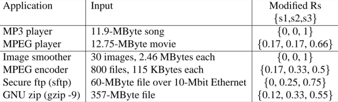
Application Input Modified Rs
s1,s2,s3
MP3 player 11.9-MByte song 0, 0, 1
MPEG player 12.75-MByte movie 0.17, 0.17, 0.66
Image smoother 30 images, 2.46 MBytes each 0, 0, 1
MPEG encoder 800 files, 115 KBytes each 0.17, 0.33, 0.5
Secure ftp (sftp) 60-MByte file over 10-Mbit Ethernet 0, 0.25, 0.75
GNU zip (gzip -9) 357-MByte file 0.12, 0.33, 0.55
Table 5: Applications, their inputs, and the grouping of run-lengths in their modified versions (assuming
CO states). We consider two streaming (top) and two non-streaming applications (bottom).
listed in the third column of table 5. The
groups in the table are defined with respect to the run-lengths delimited by the inactivity thresholds of CO. From left to right, each of the values within the braces represents the percentage of run-lengths corresponding to states 1, 2, and 3. For
example, a distribution of run-lengths of 0,0,1 means that we measured all run-lengths to be
long enough to take the disk to the sleep state in a cost-effective way. The run-length distributions
for the original versions of our applications are always 1,0,0 , i.e. no run-length is long enough
to take the disk to a low-power state.
To understand the effect of operating system prefetching, we execute experiments with and without this optimization. We use the standard prefetching policy of Linux, in which a variable-size prefetch buffer is associated with each open file. The buffer grows up to 128 KBytes, if the file is being read sequentially. It shrinks if reads are not sequential. Prefetching is done synchronously if, upon a read, the file pointer is outside of an already prefetched block and the block being requested is not in memory. Prefetching is done asynchronously if, upon a read, the file pointer is on an already prefetched block. In this case, Linux will request the next window of blocks, up to the 128-KByte limit.
The disk energy consumed by the applications is monitored by a digital power meter that sam-ples the supply voltage and the current drawn by the disk about 38K times per second. The meter provides averaged power information 3-4 times per second to another computer, which logs it for later use.
0 100 200 300 400 500 600 700 800 CO DD PA FT EO UM 0 50 100 150 200 250 300 350 400 450 CO DD PA FT EO UM Energy(J) Performance(sec) Energy MP3 Player Time Modeled Measured Disk Access Prefetching 0 20 40 60 80 100 120 140 160 180 200 CO DD PA FT EO UM 0 20 40 60 80 100 120 CO DD PA FT EO UM Energy(J) Performance(sec) Energy MPEG Player Time Modeled Measured Disk Access Prefetching 0 50 100 150 200 250 300 350 400 CO DD PA FT EO UM 0 50 100 150 200 250 300 350 400 CO DD PA FT EO UM Energy(J) Performance(sec) Energy Image Smoother Time Modeled Measured Disk Access Prefetching 0 50 100 150 200 250 CO DD PA FT EO UM 0 20 40 60 80 100 120 140 CO DD PA FT EO UM Energy(J) Performance(sec) Energy MPEG Encoder Time Modeled Measured Disk Access Prefetching 0 50 100 150 200 250 300 350 400 450 CO DD PA FT EO UM 0 50 100 150 200 250 CO DD PA FT EO UM Energy(J) Performance(sec) Energy Secure FTP Time Modeled Measured Disk Access Prefetching 0 100 200 300 400 500 600 700 800 CO DD PA FT EO UM 0 50 100 150 200 250 300 350 400 450 500 CO DD PA FT EO UM Energy(J) Performance(sec) Energy GNU Zip Time Modeled Measured Disk Access Prefetching
Figure 5: Energy and time results for MP3 player (top left), MPEG player (top right), image smoother
4.7
Experimental Results
Figure 5 presents the measured and modeled results for our applications. Each graph plots two groups of bars, disk energy (left) and CPU time (right), with results for all policies. The three leftmost bars in each group (labeled “UM”) correspond to the original, unmodified applications. From left to right, the three bars present the modeling result (adjusted, in the case of energy), the experimental result (highlighting the fraction due to actual disk accesses), and the experimental result in the presence of prefetching. All other results in each graph correspond to the transformed applications under our energy management policies. In the EO and FT results, run-lengths are extended. In the DD, PA, and CO results, run-lengths are extended and informed to the operating system. Note that we do not present prefetching results for all policies.
We computed the modeling results using the actual run-lengths observed during the appli-cations’ runs. The modeling results predict behavior in the absence of prefetching; prefetching violates the assumption that disk accesses are blocking and, thus, renders our models and instru-mentation inaccurate. We do not present modeling results for the unmodified MPEG encoder because it produces more run-lengths than our log data structure in the kernel can store.
Energy. We can make several interesting observations from these graphs. Let us start by
consid-ering the results without prefetching. First, the graphs demonstrate that our adjusted models can indeed approximate the behavior of the applications in all cases. Although the simple models’ results are not shown explicitly, we find that the adjusted models can predict energy/time more accurately than the simple models. The difference between their predictions approaches a factor of 2 in some cases, namely energy for the unmodified MP3 and MPEG players. These results suggest that modeling and/or simulation studies of device energy can lead to misleading observations.
Second, the graphs demonstrate that the application support indeed conserves a significant amount of energy in all cases. The transformation to increase run-lengths reduces energy con-sumption even under EO, an energy-oblivious policy. When we execute the modified applications in the presence of FT, energy consumption is further reduced in most cases. The exception here is
the MPEG player, for which run-lengths are exactly in the range where FT performs worse than EO. PA conserves either a little more or a little less energy than FT, as one would expect.
Exploiting run-length information provides even more gains, as shown by the DD and CO results. Modified applications under DD and CO can consume as much as 89% less energy than their unmodified counterparts, as in the case of the MP3 player. Our worst result is for gzip, for which the energy savings is 55% (CO). The average disk energy savings is 70%. The CO policy usually consumes a little more energy than DD, since run-length mispredictions may cause the disk to be idle longer than necessary under CO. The same problem is not as severe for PA (percentage-wise) because re-activations under this policy usually come from a shallower state than in CO.
Execution time. Still assuming no prefetching, we observe that the modeling results are again
accurate; they suggest the same behaviors and trends as the experimental results.
We can also observe that UM and EO exhibit roughly the same performance, showing that the overhead of extending run-lengths in the way we propose is negligible. FT and DD usually exhibit the worst performance, as one would expect. The disk re-activations are the main cause for the performance degradation under these policies. Furthermore, the figures show that PA and CO are effective at limiting performance degradation. On average, performance under these policies is 3% worse than under EO. Gzip is the application that exhibits the largest degradation, 8%. This degradation is a consequence of a few run-length mispredictions that cause disk re-activations in the critical path of the computation. This problem can be alleviated by informing slightly shorter run-lengths than we predict to the operating system or having the operating system itself provide the slack. The amount of slack cannot be too significant however, to avoid increasing the energy consumption excessively.
Prefetching. In terms of performance, prefetching has a negligible effect. The reason is that,
for non-streaming applications, our transformations operate on a large (19-MByte) buffer so any additional prefetching the operating system can perform is unlikely to make a noticeable difference. For streaming applications, the performance is mostly determined by the stream rate which is
0 50 100 150 200 250 300 350 400 CO hm CO cc DD hm DD cc FT hm FT cc EO hm EO cc 0 50 100 150 200 250 300 350 400 450 CO hm CO cc DD hm DD cc FT hm FT cc EO hm EO cc Energy(J) Performance(sec) Energy MP3 Player Time Modeled Measured Disk Access 0 20 40 60 80 100 120 CO hm CO cc DD hm DD cc FT hm FT cc EO hm EO cc 0 20 40 60 80 100 120 CO hm CO cc DD hm DD cc FT hm FT cc EO hm EO cc Energy(J) Performance(sec) Energy MPEG Player Time Modeled Measured Disk Access 0 50 100 150 200 250 CO hm CO cc DD hm DD cc FT hm FT cc EO hm EO cc 0 50 100 150 200 250 CO hm CO cc DD hm DD cc FT hm FT cc EO hm EO cc Energy(J) Performance(sec) Energy Secure FTP Time Modeled Measured Disk Access
Figure 6: Energy and time for compiler versions of MP3 player (top left), MPEG player (top right), and
sftp (bottom).
virtually independent of the performance of disk accesses. Finally, the disk access time for all applications corresponds to a small fraction of the total execution time.
In terms of energy, prefetching does have an effect on the unmodified version of three applica-tions: MP3 player, MPEG player, and gzip. These three applications access data sequentially and in small chunks in their original form. Because prefetching brings larger chunks into memory, it reduces the number of accesses that actually reach the disk, thereby reducing the energy consump-tion. Recall that a disk access consumes significantly more energy than any low-power state. This effect is not as clearly pronounced for other applications. The limited implications of prefetching is the reason why we do not present all prefetching results in our figures.
compiler-Application Phase 1 Phase 2 Phase 3 Total
MP3 player 21.1 0.2 403.2 424.5
MPEG player 7.2 0.2 98.8 106.2
Secure ftp 8.9 0.2 222.6 231.7
Table 6: Time (in seconds) spent during each phase.
based (“cc”) results for the MP3 and MPEG players (streaming applications) and sftp (a non-streaming application). We show a sampling of the amount of time spent in each phase of our compiler and runtime framework in table 6.
The results show that the energy consumption and performance of the hand-modified and compiler-based versions are nearly identical in the vast majority of cases. The framework is able to achieve these results by profiling applications for a relatively short amount of time, at most 5% of the execution time for MP3 player. This shows that our framework is able to accurately measure the disk performance without significant energy or runtime overhead, effectively manage the read buffers, and accurately predict the run-lengths.
5
Conclusions
This paper studied the potential benefits of application-supported device management for optimiz-ing energy and performance. We proposed simple application transformations that increase device idle times and inform the operating system about the length of each upcoming period of idleness. Using modeling, we showed that there are significant benefits to performing these transforma-tions for large regions of the application space. Using operating system-level implementatransforma-tions and experimentation, we showed that current non-interactive applications lie in a region of the space where they cannot accrue any of these benefits. Furthermore, we experimentally demonstrated the gains achievable by performing the proposed transformations. We also proposed a compiler framework that can transform applications automatically. Our results showed that this prototype compiler can achieve virtually the same results as when we hand-modify applications. Overall,
we found that our proposed transformations can achieve significant disk energy savings (70% on average) with a relatively small degradation in performance (3% on average). Even though our transformations target device energy management, they can potentially be combined with tech-niques that conserve processor energy. In fact, assuming that a small performance degradation is acceptable in exchange for high energy savings, processor voltage/frequency scaling may provide additional gains for our applications.
Finally, it is important to mention that, although this paper considered one particular disk, the transformations and compiler framework we propose should be directly applicable to a wide variety of disks. In fact, the runtime profiling in our compiler was designed to be used transparently across different disks. The operating system modifications we performed are also directly applicable to any disk, provided that the disk parameters are made available to the kernel.
Acknowledgements
We would like to thank the anonymous referees for comments that helped improve this paper. This research was partly supported by NSF CAREER awards CCR-0238182 and CCR-9985050.
References
[1] The Advanced Configuration and Power Interface. http://www.acpi.info/.
[2] V. Delaluz, M. Kandemir, N. Vijaykrishnan, A. Sivasubramaniam, and M. J. Irwin. DRAM Energy Management Using Software and Hardware Directed Power Mode Control. In
Pro-ceedings of the International Symposium on High-Performance Computer Architecture,
Jan-uary 2001.
[3] Fred Douglis and P. Krishnan. Adaptive Disk Spin-Down Policies for Mobile Computers.
[4] Fred Douglis, P. Krishnan, and Brian Marsh. Thwarting the Power-Hungry Disk. In
Proceed-ings of the 1994 Winter USENIX Conference, January 1994.
[5] Carla Ellis. The Case for Higher Level Power Management. In Proceedings of Hot-OS, March 1999.
[6] Xiaobo Fan, Carla Ellis, and Alvin Lebeck. Memory Controller Policies for DRAM Power Management. In Proceedings of the International Symposium on Low Power Electronics and
Design, August 2001.
[7] Jason Flinn and M. Satyanarayanan. Energy-Aware Adaptation for Mobile Applications. In
Proceedings of the 17th Symposium on Operating Systems Principles, pages 48–63,
Decem-ber 1999.
[8] Paul Greenawalt. Modeling Power Management for Hard Disks. In Proceedings of the
Con-ference on Modeling, Analysis, and Simulation of Computer and Telecommunication Systems,
January 1994.
[9] David P. Helmbold, Darrell D. E. Long, and Bruce Sherrod. A Dynamic Disk Spin-Down Technique for Mobile Computing. In Proceedings of the 2nd International Conference on
Mobile Computing, pages 130–142, November 1996.
[10] Jerry Hom and Uli Kremer. Energy Management of Virtual Memory on Diskless Devices. In
Proceedings of the Workshop on Compilers and Operating Systems for Low Power,
Septem-ber 2001.
[11] Chi-Hong Hwang and Allen C.-H. Wu. A Predictive System Shutdown Method for Energy Saving of Event-Driven Computation. ACM Transactions on Design Automation and
Elec-tronic Systems, 5(2):226–241, April 2000.
[12] A. Karlin, M. S. Manasse, L. Rudolph, and D. D. Sleator. Competitive Snoopy Caching.
[13] Kester Li, Roger Kumpf, Paul Horton, and Thomas Anderson. A Quantitative Analysis of Disk Drive Power Management in Portable Computers. In Proceedings of the 1994 Winter
USENIX Conference, pages 279–291, January 1994.
[14] Y.-H. Lu, L. Benini, and G. De Micheli. Power-Aware Operating Systems for Interactive Systems. IEEE Transactions on VLSI, 10(2), April 2002.
[15] Yung-Hsiang Lu, Luca Benini, and Giovanni De Micheli. Requester-Aware Power Reduction. In Proceedings of the International Symposium on System Synthesis, September 2000. [16] Yung-Hsiang Lu, Eui-Young Chung, Tajana Simunic, Luca Benini, and Giovanni De Micheli.
Quantitative Comparison of Power Management Algorithms. In Proceedings of the Design
Automation and Test Europe, March 2000.
[17] Yung-Hsiang Lu, Tajana Simunic, and Giovanni De Micheli. Software Controlled Power Management. In Proceedings of the IEEE Hardware/Software Co-Design Workshop, May 1999.
[18] OnNow and Power Management. http://www.microsoft.com/hwdev/onnow/.
[19] A. E. Papathanasiou and M. L. Scott. Energy Efficiency through Burstiness. In Proceedings
of the 5th IEEE Workshop on Mobile Computing Systems and Applications, October 2003.
[20] SUIF. Stanford University Intermediate Format. http://suif.stanford.edu/.
[21] A. Weissel, B. Buetel, and F. Bellosa. Cooperative I/O – A Novel I/O Semantics for Energy-Aware Applications. In Proceedings of the 5th Symposium on Operating Systems Design and
Implementation, December 2002.
[22] John Wilkes. Predictive Power Conservation. Technical Report HPL-CSP-92-5, Hewlett-Packard, May 1992.
Biographies
Taliver Heath. Taliver Heath graduated from Florida State University in 1995 with BSc degrees in
Physics and Computer Science. He went on to teach in the US Navy for 4 years, and is currently a PhD candidate in the Department of Computer Science at Rutgers University. His research interests include energy conservation and modeling of computer systems.
Eduardo Pinheiro. Eduardo Pinheiro received a BSc in Computer Engineering from PUC-Rio,
Brazil in 1996, an MSc in Computer Science from COPPE/UFRJ, Brazil in 1999, and an MSc in Computer Science from the University of Rochester in 2000. He is currently a PhD candidate in the Department of Computer Science at Rutgers University. His main research interests include operating systems and energy conservation in computer systems.
Jerry Hom. Jerry Hom is a PhD candidate at Rutgers University in the Computer Science
De-partment. He received a BSc degree in Electrical Engineering and Computer Science from the University of California, Berkeley. His recent research interests include compilers, languages, optimizations, and energy and power reduction techniques for computer systems.
Ulrich Kremer. Ulrich Kremer is an Associate Professor in the Department of Computer Science
at Rutgers University. His research interests include advanced optimizing compilers, performance prediction models, compiler optimizations for location-aware programs on mobile target systems, and compiler support for power/energy management. He has been a Principal Investigator and Co-Investigator on several NSF and DARPA funded projects, including an NSF CAREER award. He received his PhD and MS in Computer Science from Rice University in 1995 and 1993, respec-tively, and his diploma in Computer Science from the University of Bonn, Germany, in 1987. He is a member of the ACM.
Ricardo Bianchini. Ricardo Bianchini received his PhD degree in Computer Science from the
University of Rochester in 1995. From 1995 until 1999, he was an Assistant Professor at the Federal University of Rio de Janeiro, Brazil. Since 2000, he has been an Assistant Professor in the Department of Computer Science at Rutgers University. His current research interests include
the performance, availability, and energy consumption of cluster-based network servers. He has received several awards, including the NSF CAREER award. He is a member of the IEEE and the ACM.