Study on Machine Learning and Deep Learning Methods for Cancer Detection

(1)

Study on Machine Learning and Deep Learning Methods for

Cancer Detection

Bhagyasri, Bhavanishree P.N, Madan Kumar S, Gagan.S.Bharadwaj, Dr Dayanand. P Department of ISE

Jss Academy of Technical Education, Bangalore Abstract

Cancer causes death of about million people every year. Cancer is the frequently recognized and is the major reason of death in men and women. Cancer is a group of diseases involving abnormal cell growth which will spread to other parts of the body. Colonography makes use of low dose radiation Computed tomography (CT) scanning to get an internal view of the cancer tumors making use of special x-ray machine to view tumors. Radiologists examine these images to find tumor like structure using computer tools. As CT Colonography image contain noise such as lungs, small intestine, instruments during image capturing. Cancer occurrence can be detected mainly using shape feature; eliminating shapes similar to tumor is challenging. Hence, to tackle above issues, image processing techniques are used by applying deep learning algorithm- Convolution Neural Network (CNN) and the results are compared with classical machine learning algorithm. The analysis is done with classical machine learning algorithms - Random Forest algorithm (RF) and k-nearest neighbour algorithm (KNN) by extracting texture feature - Local binary pattern (LBP) and shape feature - Histogram oriented gradient (HOG) for comparison.

Keywords: Support Vector Machine (SVM), Convolution Neural Network (CNN), Deep Belief Networks (DBN), K-nearest neighbour (KNN)

INTRODUCTION

Cancer is caused because of abnormal growth of cells. There are various types of cancer such as breast cancer, colon cancer, lung cancer, blood cancer. Some of the symptoms are change in bowel habits,

blood-tinged saliva, diarrhoea,

constipation, blotting or pain. Some of the methods used in treatment and detection are Support Vector Machine (SVM), Convolution neural network, k-nearest neighbour method, and Random forest method. SVM is utilised for classification and regression of images. CNN eliminates the need for manual feature extraction, the features are learned by the CNN. Random forest provides correct prediction of class for most part of the data. The k-nearest neighbour classifier is known as simple machine learning/image classification methods. Image processing techniques are

used by applying deep learning methods Convolution Neural Network (CNN) and the results are compared with classical machine learning methods. CNN makes use of many methods for input data, and during processing it will solve the problems such as spreading up noise and signal distortion.

Types of Deep Learning Methods

 Deep Boltzmann Machine (DBM)  Deep Belief Networks (DBN)  Stacked Auto-Encoders

 Convolution Neural Network (CNN)

Deep Boltzmann Machine (DBM)

Boltzmann Machine is also known as stochastic Hopfield network with hidden units. DBM is a kind of stochastic Recurrent Neural Network (RNN). The first neural networks that have ability to

(2)

learn internal representations and they also solve difficult problems. Learning can be made efficient only when connectivity is properly checked which is useful for practical problems. To show better representations of input structures, DBN‟s and deep convolutional neural networks uses interference and training process in bottom-up and top-down. DBM‟s limits their performance and functionality because of their slow speed.

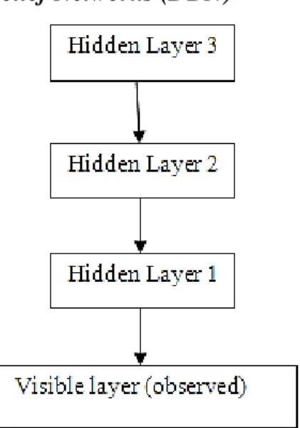
Deep Belief Networks (DBN)

Fig 1. Overview of Deep Belief Networks

In the above Figure the arrow represent directed connections in the model that the net represents. DBN is a generative graphical model that has several layers of hidden units, where there exists connection between layers but there is no connection between each layer units. DBNs can be seen as a form of simple, unsupervised networks. Each hidden layer will serve as a visible layer for the next.

Stacked Auto-Encoders

A stacked auto-encoder is a neural network with multiple layers of sparse autoencoders where the outputs of one layer are connected to the input of the next layer. Greedy layer-wise training is used to gain good parameters for stacked auto

encoder. This encoder will make use of all the advantages of any deep network of larger expressive power. Further it collects a useful part-whole decomposition of the input.

Convolutional Neural Network (CNN)

A convolutional neural network (CNN) is

a deep learning and feed-forward artificial neural networks. For an analyzing visual imagery purpose cnn is successfully used. These are also known as space invariant

artificial neural networks (SIANN),

depending on respective of shared-weights

architecture and also translation invariance

characteristics.

In between neurons there exists a

connectivity pattern which matches the

organization of the animal visual cortex.

Only in a confined region of the visual

field called as the receptive field

Individual cortical neurons respond to

stimuli. The particular fields of different neurons partially lap over so that they can cover the complete visual field.

A CNN contains layers like input layer,

output layer and also many hidden layers.

The hidden layers of a CNN contain convolutional layers, pooling layers, fully connected layers and normalization layers. Convolutional layers appeal a convolution operation for the input, and then the result is passed to the next layer. The acknowledgement of an individual neuron to visual stimuli is done through the convolution emulates.

Convolutional layer(CL)

As like other layers CL will receive the input then trains the forms in some way and then the output of this train form is used as input to the next layer. This is known as convolution operation. Convolutional layer are able to detect the patterns. For each convolutional layer we need to specify the number of filters the

(3)

layers should have. Filters are used to detect the patterns. One type of pattern that the pattern will detect could be edges and images. Hence this filter is called edge detector. Some filters will detect corners some may detect circles and others may detect squares.

Example: Suppose we have CNN which is accepting images of handwritten digits and network is classifying them into their respective categories. A filter could be taken as small matrix for this we will decide the number of rows and number of columns. The values in the matrix are initialized with random numbers. Now we want the layer to contain filter of size 3 by 3.when the input is received by the convolutional layer the filter will slide over each 3*3 set of pixels from input. It will slide until every 3*3 block of pixels from entire image this sliding is called as convolving.

Pooling layer

Further major concept of CNN is polling. It is an arrangement of non-linear down-sampling. Max pooling is the common among many non-linear functions to apply polling. The input image is split into a set of non-overlapping rectangles and, then for each such sub-region, it outputs the maximum.

The objective is that the exact location of a feature is not as important as its rough location comparative to other features. In a CNN architecture it is usual to put a pooling layer frequently among sequential convolutional layers. An another form of translation invariance is provided through polling operation.

On every depth slice of the input, pooling layer is used separately and changes its size spatially. Commonly used pooling layer filters is of size 2x2 which is applied with a stride of 2 down samples at every

depth slice in the input by 2 along both width and height, discarding 75% of the activations/actions. In this, each max operation requires 4 numbers. The depth dimension remains unvarying.

ReLU layer

ReLU is the contraction of Rectified

Linear Units. Non-saturating activation function is applied to this layer. Whenever the function is less than zero it gives zero. If the function is greater than zero it remains as it is. Hence it is used to remove the negative part of the function.

f(x) = 0 for x <0 x for x >=0 Fully connected layer

After many convolutional and max pooling layers, fully connected layer with the effective reasoning in the neural network is done.

Fully connected layer have neurons which have the link to all actions done in the last layer, as in frequent neural networks. Their actions can therefore be determined with a matrix multiplication along with a bias offset.

Loss layer

This layer is used to specify how the network training corrects the difference between the predicted and true labels and is normally the final layer the loss layer is

used. Softmax loss is used to identify a

single class of K mutually exclusive

classes. To identify K independent

probability values Sigmoid

cross-entropy loss is used . For reverting to

real-valued labels Euclidean loss is used.

Advantages of CNN

1. CNN eliminates manual feature extraction, since features can be learned using CNN.

2. Automatic features extraction for the given task.

(4)

 Random forest (RF)

 Support vector machine (SVM)  K-Nearest Neighbour (KNN)

Random Forest

Random Forest Algorithm is one of the most popular Supervised Classification Algorithm. It creates more number of decision trees to form a Forest. Unlike, Decision tree Algorithm in Random Forest Algorithm, identifying the root node and splitting the feature nodes will take place randomly.

Pseudocode

The Pseudocode is divided into two stages. 1. Pseudocode to create Random Forest. 2. Performs Prediction from created RF classifier.

Pseudocode to create Random Forest

Step 1: Out of „m‟ features randomly select „k‟ features that is k<m.

Step 2: Using the Best split point approach, compute the node „d‟ among „k‟ features.

Step 3: Split the node into daughter nodes using Best split approach.

Step 4: Iterate steps 1 to 3 until leaf node is obtained.

Step 5: Iterate steps 1 to 4 to create „n‟ number of decision trees.

Random Forest prediction Pseudocode

Step 1: Input the test data/test feature to the randomly created decision trees of Random Forest to predict the outcome and store the result.

Step 2: Obtain the votes for each predicted target.

(5)

Step 3: From the Random Forest Algorithm, the more number of predicted target/votes is considered as final output.

The Random Forest Algorithm is illustrated in the below figure 3:

Fig: 3 Advantages of Random Forest

1. Overfitting problem does not occur when RF algorithm is used for classification task.

2. It is used for both Regression and Classification task.

3. It is also used for feature engineering. 4. The Classifier of Random Forest Algorithm will handle the missing values.

Application

1. Banking 2. Medicine 3. Stock Market

4. E-commerce

Support Vector Machine

In SVM an infinite-dimensional space is used for classification and regression by constructing hyperplanes or set of hyperplanes. Consider Support vector machine for linearly separable binary sets. Let us consider two features x1 and x2 and we want to separate the elements. We have circles and squares. Here the objective is to draw a hyperplane that divides all training vectors in two classes as shown in Fig 4.

(6)

Scenario 1: In this scenario that there is only one hyperplane which is given by an equation and it classifies the all the

elements correctly. Distance between point and hyperplane is determined by Z.

Fig 5

Z=| → |

‖→‖ ‖→‖

Where, → is the input value and → is the vector of weights.

Scenario 2: In this scenario there are two hyperplanes which can classify all the elements correctly. From both the classes which will leave maximum hyperplane we will consider that hyperplane to classify the classes. Point and the hyperplane distance is determined by Z1 and Z2 as shown above. Here Z2 > Z1 so we will consider Z2. g( → is greater than or equal

to 1 for all input values that belongs to class 1 and g( → is less than or equal to 1 for all input vectors that belongs to class 2 as shown in Fig 4 and Fig 5.

If g( → >= 1 where, ¥→€ class 1 g( → <= 1 where, ¥→€ class 2 The total margin is computed by

‖→‖ + ‖→‖ = ‖→‖ .Minimizing this term will maximize the separability

(7)

KNN stands for K-nearest neighbours algorithm, this algorithm is mainly used for pattern recognition. For classification and regression KNN uses method called non-parametric. The input depends on both classification and regression but the output depends on either of it i.e., classification or regression.

KNN Classification: The output of the classification is the class membership. KNN objects are classified by neighbours. If k = 1, then the object is allocated to the class of that single nearest neighbour. KNN-Regression: The property of value for an object is the output of the regressions. This is the mean value of the k-nearest neighbour.

KNN is of two types when it comes to learning,

1: Instance-based learning, 2: Lazy learning.

The functions in KNN are approximated locally and computations are deferred based on classification.

KNN algorithm is the simplest of all other algorithms when it comes to machine learning.

KNN Pseudocode for Classification 1. Compute “D(a, ai)” i =1, 2, ….., n; where D represents the Euclidean distance between the points.

2. All n Euclidean distance computed arrange in increasing order.

3. Consider the first „k‟ distances from the list where k is +ve integer.

4. Corresponding to „k‟ distances identify „k‟ points.

5. Among „k‟ points ki represents the number of points held to the ith class i.e. k ≥ 0.

6. If ki>kji ≠ j then place „a‟ in class i.

Advantages

1. Implementation is simple.

2. Execution is fast for small training datasets.

3. Does not require knowledge about the structure of data.

4. Retraining the model is not necessary if new data is added to the existing training set.

Limitations of KNN Algorithm:

1. Requires more space if the training set is large.

2. Requires more time for testing, because for each test data a distance is calculated between test data and all training data.

COMPARATIVE STUDY AND RESULT ANALYSIS

Properties CNN RF KNN SVM

Used for Recognition,Visualizat

ion and Segmentation of images. Classification and Regression. Image classification. Classification and Regression analysis.

Advantages Automatic features

extraction for the given task. It gives more correct classifier for many datasets Robust to noisy training data.

Mostly used for pattern recognition.

Disadvantages They do not encode

position and

orientation of the object into their predictions. Prediction process using RF is time-consuming. It is a lazy learner ie, it will not learn

anything from

training data and it takes advantage of training data itself for classification.

It will take long training time for large datasets.

(8)

A deep learning algorithm takes more time to train compared to machine learning because deep learning algorithm contains many parameters so it takes longer time to train. This will reverse on testing time. Deep learning algorithm takes short time to run, whereas if we equate this with

KNN, on increasing the size of the data test time also increases. Deep learning algorithms attempts to gain effective features from data. Performance of deep learning is good compared to other learning algorithms as shown in the graph 1.

Graph 1: deep learning vs older learning algorithms

Accuracy of CNN is more compare to other algorithms such as KNN, Random Forest and SVM as shown in graph 2.

Graph 2: Accuracy vs Training examples

CONCLUSION

Deep learning is a part of machine learning. It is nothing but a machine learning and operates in a same way, but its effectiveness is distinct. Basic machine learning models do become moderately fine at whatever their function is. If an ML

algorithm does not give an accurate

prediction, then some

adjustments/modifications should be made. But deep learning algorithms has an ability to determine correct prediction or not by their own. Hence Deep learning Algorithms have more accuracy and

0.84 0.86 0.88 0.9 0.92 0.94 0.96 0.98 500 2000 5000 10000 15000 RF CNN KNN SVM

(9)

performance compare to machine learning Algorithms.

REFERENCES

1. S. A. Karkanis, D. K. Iakovidis, D. E. Maroulis, D. A. Karras, and M. Tzivras, “Computer-aided tumor detection in endoscopic video using color wavelet features,” IEEE Trans. Inf. Technol. Biomed., vol. 7, no.3, pp. 141–152, Sep. 2003.

2. S. Bae and K. Yoon, “Polyp detection

via imbalanced learning and

discriminative feature learning,” IEEE Trans. Med. Imag., vol. 34, no. 11, pp. 2379–2393, Nov. 2015.

3. S. Park, M. Lee, and N. Kwak, “Polyp detection in colonoscopy videos using deeply-learned hierarchical features,” Seoul Nat. Univ., 2015.

4. Yann Lecun, "Deep Learning," NATURE, vol. 521, Mei 2015.

5. A. Krizhevsky, I. Sutskever, and G. E. Hinton, “Imagenet classification with deep convolutional neural networks,” in Advances in neural information processing systems, 2012, pp. 1097– 1105.

6. Y. Jia, E. Shelhamer, J. Donahue, S. Karayev, J. Long, R. Girshick, S. Guadarrama, and T. Darrell, “Caffe: Convolutional architecture for fast feature embedding,” arXiv preprint arXiv:1408.5093, 2014.

7. Y. Jia, E. Shelhamer, J. Donahue, S. Karayev, J. Long, R. Girshick, S. Guadarrama, and T. Darrell, “Caffe: Convolutional architecture for fast feature embedding,” arXiv preprint arXiv:1408.5093, 2014.

8. A. Krizhevsky, I. Sutskever, and G. E. Hinton, “Imagenet classification with deep convolutional neural networks,” in Advances in Neural Information Processing Systems 25, F. Pereira, C. J. C. Burges, L. Bottou, and K. Q. Weinberger, Eds. Curran Associates,

Inc., 2012, pp. 1097–1105.

9. K. He, X. Zhang, S. Ren, and J. Sun, “Deep residual learning for image recognition,” in Proceedings of the IEEE Conference on Computer Vision and Pattern Recognition, pp. 770-778, 2016.

10.A. Krizhevsky, I. Sutskever, and G.E. Hinton, “ImageNet classification with deep convolutional neural networks,” in Advances in neural information processing systems, pp. 1097-1105, 2012.

11.http://www.deeplearningbook.org/cont ents/convnets.html

12.Taigman, Y., Yang, M., Ranzato, M.A. and Wolf, L., 2014. Deepface: Closing the gap to human-level performance in face verification. In Proceedings of the IEEE Conference on Computer Vision and Pattern Recognition (pp. 1701-1708).

13.C. Szegedy, W. Liu, Y. Jia, P. Sermanet, S. Reed, D. Anguelov, D. Erhan, V. Vanhoucke, and A. Rabinovich, “Going Deeper with Convolutions,” 2014.

14.Y. Guo, Y. Liu, A. Oerlemans, S. Wu, and M. S. Lew, “Author‟s Accepted Manuscript Deep learning for visual understanding: A review To appear in: Neurocomputing,” 2015.

15.Shuangbao Shu, Jiarong Luo, Binxuan Sun, Nan Yu College of Science, Donghua University Shanghai, China [email protected] “Color Images Face

Recognition Based on

Multi-classification Support Vector Machine “ The 5th International Conference on Computer Science & Education Hefei, China. August 24–27, 2010.

16.Lavanya K1, Shaurya Bajaj2, Prateek Tank3, Shashwat Jain4 1 Department of Software Systems/SCOPE 2 UG Scholars, Computer Science and Engineering VIT University. Vellore, India.