IMPROVED UNDERSTANDING OF SUBSURFACE HYDROLOGY IN VARIABLE SOURCE AREAS AND ITS IMPLICATIONS FOR WATER
QUALITY
A Dissertation
Presented to the Faculty of the Graduate School of Cornell University
In Partial Fulfillment of the Requirements for the Degree of Doctor of Philosophy
by
Helen Elisabeth Dahlke January 2011
IMPROVED UNDERSTANDING OF SUBSURFACE HYDROLOGY IN VARIABLE SOURCE AREAS AND ITS IMPLICATIONS FOR WATER
QUALITY
Helen Elisabeth Dahlke, Ph. D. Cornell University 2011
Variable source areas (VSAs) are hot spots of hydrological (saturation-excess runoff) and biogeochemical processes (e.g. nitrogen, phosphorus, organic carbon cycling) in the landscapes of the northeastern U.S. Despite the substantial research conducted in the past 50 years, there is still process understanding to be gained on how VSA connect with the surrounding area, how this interaction influences surface and subsurface runoff generation and chemical transport and how these processes can be captured in ungaged basins using watershed models. To determine the controls on VSA formation and connectivity, a 0.5 ha hillslope was instrumented (trenched) in the southern tier of New York, U.S. Water flux from different soil layers in the trench and upslope water table dynamics were recorded for 16 events and isotopic and geochemical tracers were measured during five events. In conjunction with the surface and bedrock topography these measurements allowed detailed characterization of the subsurface storm flow response within the VSA. Analysis revealed that the most important control on storm flow response was antecedent moisture. During events with dry antecedent conditions subsurface flow was dominated by percolation through the fragipan (i.e. cracks and macropores). Flow from below the fragipan showed a constant flow rate (0.8 mm/h), which was independent of storm size and antecedent moisture. Under wet antecedent conditions hydrological connectivity increased and
subsurface flow is dominated by lateral flow through the soil atop the fragipan. During these events flow contributing slope length to the trench was five to tenfold increased. Thus, pollutant and nutrient transport from a greater distance has to be considered in water management during events with wet antecedent conditions. Application of the empirical Soil Conservation Service Curve Number method showed that discharge volumes were generally well predicted but revealed that for continuous predictions of VSA dynamics more conceptually coherent solutions need to be developed that consider the effect of antecedent moisture on runoff generation. This research shows that indirect indicators such as the average water table depth, the base flow rate prior to events or water balance estimates of the soil water content can be incorporated into watershed models to improve predictions.
BIOGRAPHICAL SKETCH
Helen Elisabeth Dahlke was born in Leipzig, Germany, in 1978. After she graduated from Alexander-von-Humboldt-Gymnasium in Leipzig in 1997, she enrolled at the Friedrich-Schiller-University in Jena, Germany and received in 2004 a M.Sc. in Geography (Diplom-Geograph), with minors in Geology and Ecology. During her time at Friedrich-Schiller-University in Jena she worked and traveled in South Africa, and became interested in catchment hydrology and hydrological systems that are impacted by environmental changes across spatial and temporal scales. After finishing her M.Sc. in Germany she continued working in catchment hydrology projects in Eastern Europe and Sweden and gained experience in geostatistical, field measurement, and geophysical methods, as well as GIS and modeling. In January 2007, Helen joined Cornell University to start her Ph.D. program at the Department of Biological and Environmental Engineering.
This dissertation is dedicated to my parents Johanna and Ulrich Dahlke, my sister Franka, my grandparents Elfriede and Heinz Weinhold, to my partner Anthony and my closest friend Verónica,who have encouraged me, loved and believed in me during
ACKNOWLEDGMENTS
This work would not have been possible without the dedication and support of numerous people and funding sources. First of all I would like to thank my advisor Tammo Steenhuis and my committee members Larry Brown and Jery Stedinger for their steady support, patience, constructive critique and the many hours of help and discussion they offered during the last four years. I especially want to thank Tammo Steenhuis for giving me the opportunity to join the graduate program at Cornell University and to become a member of his diverse and multi-national research lab.
This research was mainly funded through the U.S. Department of Agriculture and the Cooperative State Research, Education and Extension Service (CSREES) by the grant “Improving the Transport Component of the P-Index for Nutrient Management Plans in the Northeast “. Beyond this, I gratefully acknowledge the B.K. Krenzer and N.G. Kaul scholars for their financial support of this research.
This field research would not have been a success without the help of my many colleagues and friends who volunteered unconditionally for many times. I especially would like to acknowledge Zachary Easton who spent many hours planning, digging and discussing site instrumentation, data analysis and data interpretation. Beside him I owe special thanks to Steve Lyon who suggested to come to Cornell University as well as Chris Berry, Brian Buchanan, Carla Ferreira, Joshua Faulkner, Daniel Fuka, Christian Guzman, Ri Young Ko, Becky Marjerison, Veronica Morales, Sheila Saia, Anthony Salvucci, Eric White, and Wei Zhang. I am also grateful to M. Todd Walter, Larry Goehring and Brian Richards from the Soil and Water Lab for advising me and discussing the many technical and instrumental challenges faced during my PhD.
Finally, I want to cordially thank my family, especially my mother Johanna and my partner Anthony, for their support, love and encouragement over years.
TABLE OF CONTENTS
BIOGRAPHICAL SKETCH ... iii
DEDICATION ... iv
ACKNOWLEDGEMENTS ... v
TABLE OF CONTENTS ... vi
LIST OF FIGURES ... vii
LIST OF TABLES ... xi
LIST OF ABBREVIATIONS ... xiii
LIST OF SYMBOLS ... xvi
CHAPTER 1: INTRODUCTION ... 1
CHAPTER 2: DISSECTING THE VARIABLE SOURCE AREA CONCEPT – FLOW PATHS AND WATER MIXING PROCESSES ... 16
CHAPTER 3: A FIELD TEST OF THE VARIABLE SOURCE AREA INTERPRETATION OF THE CURVE NUMBER RAINFALL-RUNOFF EQUATION ... 57
CHAPTER 4: MODELING VARIABLE SOURCE AREA DYNAMICS IN A CEAP WATERSHED ... 87
CHAPTER 5: A WEB-BASED DECISION SUPPORT SYSTEM TO FORECAST HYDROLOGICALLY SENSITIVE AREAS ... 121
APPENDIX A: ESTIMATION OF SOIL WATER CONTENT AND SOIL DEPTH IN A TRENCHED HILLSLOPE USING GROUND PENETRATING RADAR .... 150
LIST OF FIGURES
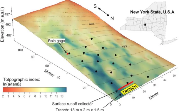
Figure 2.1: Location of study hillslope in central New York State, U.S.A.. Black dots indicate locations of water level loggers. The red dashed line is indicating the
watershed boundary for the trench contributing area as derived from surface
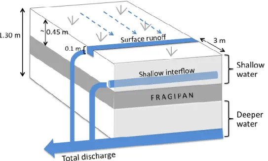
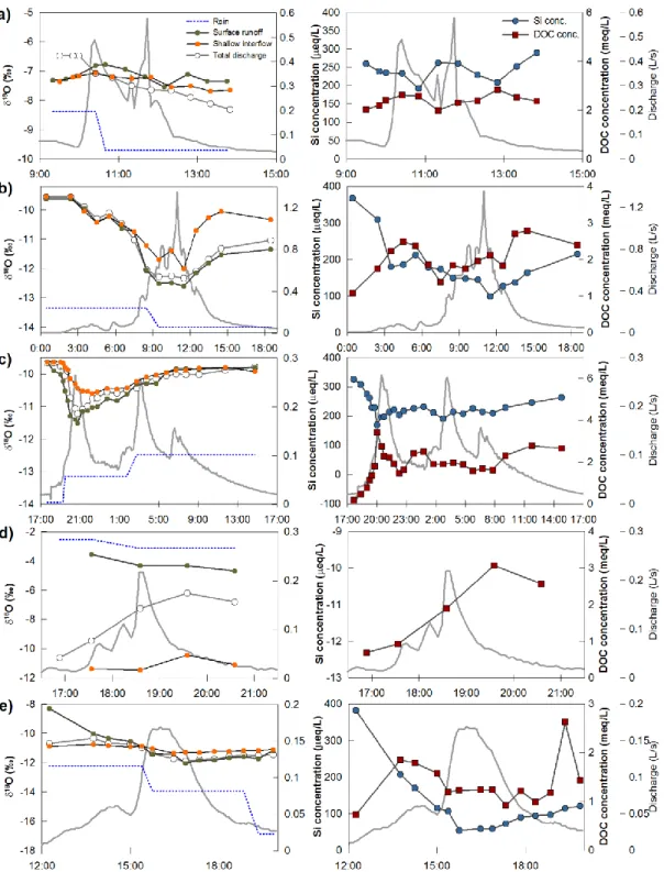
topography. ... 21 Figure 2.2: Schematic layout of the trench instrumentation and collectors of different flow components (surface runoff, shallow interflow, total discharge). For the chemical hydrograph separation water coming to the trench is separated into shallow water from top the fragipan and deeper water from below the fragipan. ... 23 Figure 2.3: Hillslope instrumentation and depth to fragipan survey. Locations of water level loggers are indicated by black dots. A sand lens (red dashed line) was detected with ground penetrating radar and confirmed with particle distribution data of soil samples. ... 24 Figure 2.4: (a) Rainfall hyetograph and cumulative rain for the study period from October 2009 until May 2010 (excluding the frost period). (b)Total discharge (L/s) measured in the trenched hillslope. (c) Time series of the average depth to the water table in the hillslope, and (d) of the saturated hillslope fraction, derived when the water table was 10 cm below the soil surface. ... 33 Figure 2.5: Time series data of δ18O (‰) ratios observed in the surface runoff,
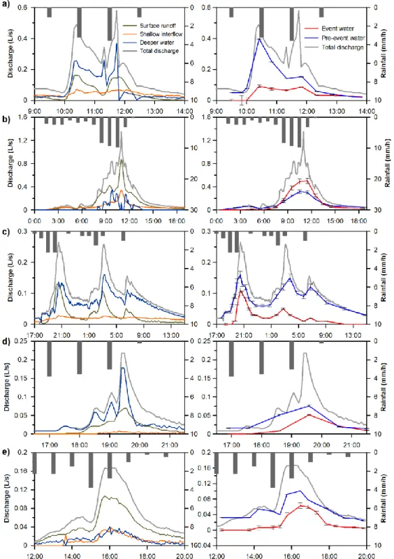
shallow interflow and total discharge (left graphs), and Si (μeq/L) and DOC (meq/L) concentrations measured in the total discharge (right graphs) for the events on 24 October 2009 (a), 28 October 2009 (b), 2 December 2009 (c), 17 April 2010 (d), and 26 April 2010 (e). Bulk sample rain δ18O data are indicated by blue dotted lines. For the five storms a two-component (one tracer) hydrograph separation was performed. 36 Figure 2.6: Time series of measured surface runoff, shallow interflow, total discharge, and hourly rainfall (left graphs), and the two-component, one-tracer (δ18O)
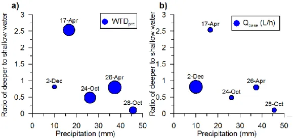
hydrograph separation into event and pre-event water (right graphs) for the events on 24 October 2009(a), 28 October 2009 (b), 2 December 2009 (c), 17 April 2010 (d), and 26 April 2010 (e). Uncertainty bars represent the propagation of a 10% flow error and the double analytical precision of end-member tracers. ... 40 Figure 2.7: (a) Influence of total precipitation and depth to the water table prior to storm events (WTDpre) on the ratio of deeper water to shallow water, and (b)
influence of total precipitation and the base flow rate prior to storm events (Qbase) on the ratio of deeper water to shallow water for the five storm events. Bigger bubbles indicate higher values. ... 43 Figure 2.8: DOC versus Si mixing diagrams for the storm events on 24 October (a) and 2 December 2009 (b). Concentrations in the total discharge, surface runoff and shallow interflow are shown as black, green and orange solid circles respectively. Purple squares indicate the chemistry of free water purged from piezometer wells before (if water was present) and after each storm event. See Figure 2 and 9 for the location of piezometers in relation to the trench and saturated area in the hillslope. .. 44
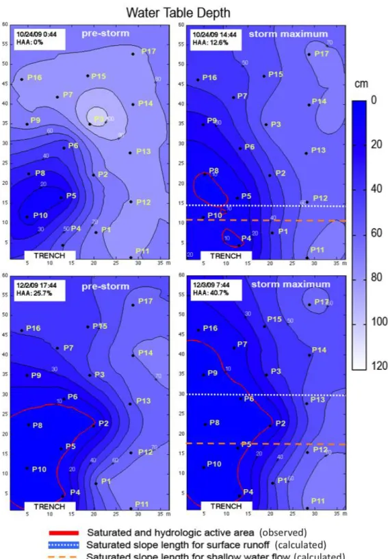
Figure 2.9: Pre-storm and maximum saturated area extend (highlighted with the red solid line) observed during the 24 October (top) and 2 December (bottom) storm event. Saturated and runoff generating areas were derived when the water table was above 10 cm below the soil surface. The white dotted and orange dashed line indicate the flow contributing, saturated slope length for each event, which was calculated based on observed surface runoff and shallow interflow volumes respectively. ... 45 Figure 3.1: Location of study hillslope in central New York State, U.S.A. Black dots indicate locations of water level loggers. ... 62 Figure 3.2: Schematic layout of the trench instrumentation and collectors of different flow components (surface runoff, shallow interflow) and total discharge. ... 64 Figure 3.3: Rainfall and total discharge time series (a), dynamics of the average depth to the water table in the hillslope (b), and the fractional saturated area (c) recorded in the trench hillslope for the study period from 06 October 2009 until 31 May 2010. Measurements were discontinued from 9 December 2009 until 31 March 2010 due to snow cover and frozen soils. ... 68 Figure 3.4: Linear regressions between predicted saturated areas using the VSA
interpretation of the SCS-CN method and observed average saturated area extends, which were derived for different water table depths below the soil surface. Best agreement is achieved if the regression line approaches closely the 1:1 line. RMSE is the root-mean-squared error and E shows the Nash-Sutcliffe coefficient (Nash and Sutcliffe, 1970). ... 72 Figure 3.5: Relationship between (a) the initial abstraction or amount of water required to initiate runoff and the average depth to the water table in the hillslope prior to each storm event, and (b) the initial abstraction and base flow observed within the 24-hour period prior to each storm event. ... 74 Figure 3.6: Comparison of observed initial abstraction and calculated initial
abstraction if the watershed storage equals S=15.5 cm. The estimated initial abstraction shows negative values for events with wet antecedent conditions when discharge was greater than rainfall inputs. For these events the observed Ia was set to zero. ... 75 Figure 3.7: Relationship between total observed saturation-excess runoff and the product of effective precipitation times the average fractional saturated hillslope area as observed if the water table was at 5 cm (a), 10 cm (b), 15 cm (c), or 20 cm (d) below the soil surface. Inserts show data pairs for 15 storm events excluding the largest storm on 28 October 2009. ... 77 Figure 4.1: Location of Town Brook watershed in the Catskill Mountains, New York State (upper left). The left panel shows locations of water level loggers (black dots) considered in and excluded from this analysis (white dots) and the soil topographic index (STI) for the hillslope. The right panel shows the event-averaged depth to the water table for each water level logger underlain by a map of the wetness classes (as reclassified from the STI). ... 92 Figure 4.2: (a) Fractional runoff contributing area (Af) and (b) average depth to water table of all sampling locations for the event analysis period March – September 2004.
Circles indicate the 14 selected events. The horizontal, dashed line in (b) indicates the threshold water table depth above which runoff generation is initiated. ... 102 Figure 4.3: (a) Precipitation, and (b) observed and predicted streamflow for the water balance model from January 2003 to December 2004. ... 105 Figure 4.4: Correlation of the soil topographic index (STI) and average event water table depth of each sampling location (a), and wetness class vs. average water table depth based on all data loggers located in any wetness class. ... 107 Figure 4.5: Average, minimum and maximum water table depths shown for each wetness class for events from 05 March until 27 May 2004. The vertical lines show the maximum range of wetness classes contributing runoff during this storm event as predicted with the original SCS-CN equation (dotted line) and the revised SCS-CN runoff equation (black line). The thin, horizontal dashed lines show the threshold water table depth above which the sampling locations indicate that runoff generation is initiated. ... 110 Figure 4.6: Average, minimum and maximum water table depths shown for each wetness class for events from 27 July until 28 September 2004. The vertical lines show the maximum range of wetness classes contributing runoff during this storm event as predicted with the original SCS-CN equation (dotted line) and the revised SCS-CN runoff equation (black line). The thin, horizontal dashed lines show the threshold water table depth above which the sampling locations indicate that runoff generation is initiated. ... 111 Figure 5.1: Integrated system components of the HSA-DSS. ... 126 Figure 5.2: Sample message of the Global Forecast System (GFS) Model Output Statistic (MOS) for the Ithaca, NY climate station. Elements used in the forecast module of the HSA-DSS are FHR = forecast hour, X/N = daytime max, nighttime min temperature, P24 = 24-hr probability of precipitation, and Q24 = 24-hr quantitative precipitation forecast. ... 128 Figure 5.3: Presentation tier and start page of the HSA-DSS. ... 131 Figure 5.4: Presentation tier of the HSA-DSS. Red areas show HSA predicted with the hydrologic assessment tool. A daily update of forecasted weather conditions and HSA dynamics in Salmon Creek watershed is given in the top of the right frame. ... 131 Figure 5.5: Daily updated status report showing forecasted rainfall amounts, rainfall probability and expected percent area of the watershed that could saturate or generate runoff. ... 132 Figure 5.6: Location and characteristics of Salmon Creek watershed. ... 133 Figure 5.7: Precipitation (a), and measured and modeled discharge (b) for the water balance model of Salmon Creek watershed from July 2006 to January 2010. ... 136 Figure 5.8: Monthly probability of saturation for Salmon Creek watershed. For each month the fraction is shown that saturates or generates runoff in more than 50% (red areas), 25% (yellow areas), 10% (green areas), and 0% (white areas) of the rainfall events. ... 140
Figure A.1: Propagation paths of electromagnetic waves in a soil with two layers of contrasting dielectric permittivity (ε1 and ε2). Tx and Rx are the transmitter and receiver respectively. ... 154 Figure A.2: Schematic layout of wave arrivals when performing a common-midpoint (CMP) or wide angle reflection and refraction (WARR) measurement. The ground wave can be identified as a wave with a linear move out starting from the origin of the x-t plot. In the slope equations, c is the electromagnetic velocity of air and x is the antenna separation. ... 157 Figure A.3: GPR profile acquired in the trenched hillslope with a PulseEkko system, 200 MHz antennas in 1 m FO mode. The profile is shown after completion of data processing. The orange, red and green lines show the air wave, ground wave and reflected wave respectively. ... 162 Figure A.4: CMP profile acquired in the trenched hillslope with a PulseEkko system, 200 MHz antennas. The orange, red and green lines indicate the air wave, ground wave and reflected wave respectively and associated velocities. ... 163 Figure A.5: Estimation of radar velocity by fitting a hyperbola to a point reflector in the subsurface. Depth to hyperbola is D = 0.6 m. ... 163 Figure A.6: Map of the soil depth in the trenched hillslope estimated from GPR
profiles (PulseEkko system, 200 MHz antennas, 1 m FO) using the reflected wave. Black dots indicate the location of water level loggers. ... 164 Fig. A.7: Influence of soil water content on arrival times of the air wave (orange) and ground wave (red). ... 165 Figure A.8: Map of the soil water content in the trenched hillslope estimated from GPR profiles (PulseEkko system, 200 MHz antennas, 1 m FO) using the ground wave method and the empirical equation of Topp et al. (1980). Black dots indicate the location of water level loggers. ... 167 Figure A.9: (a) Regressions of gravimetrically estimated soil water contents versus the square root of the apparent relative permittivity (εa) estimated with TDR (open circles) and the GPR ground wave method (solid circles) respectively. (b) Regressions of volumetric soil water content (θv) determined from soil samples versus θv estimated with TDR (open circles) and the GPR ground wave method (solid circles). θv-GPR, θv-TDR, and θv-soil are soil water contents estimated with the GPR ground wave method, TDR and from soil samples respectively. ... 169
LIST OF TABLES
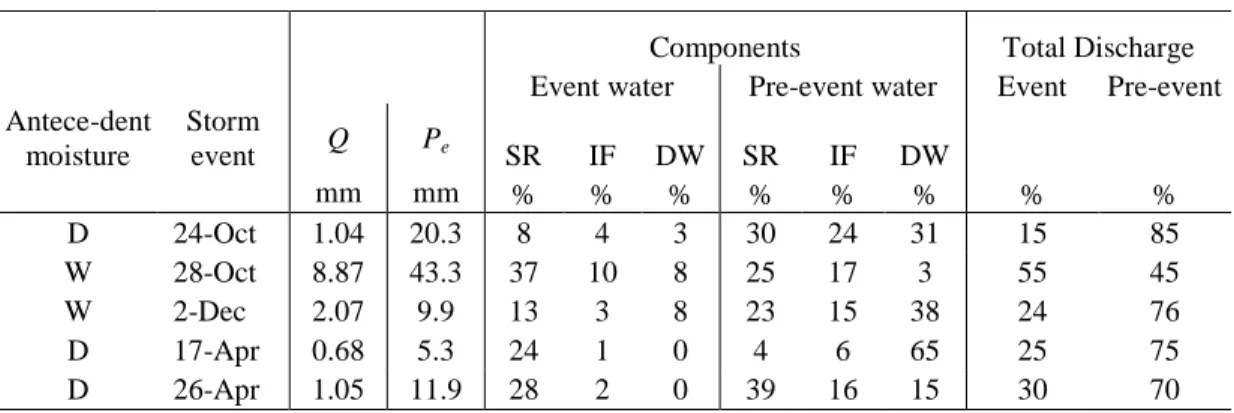
Table 2.1: Hydrometric characteristics for the five storm events presented in this study. ... 32 Table 2.2: Solute concentrations and isotopic values for the end-members used in the two-component hydrograph separation model. End-members are averaged from multiple measurements taken during base flow conditions prior to storm events. Statistical moments of tracer signals summarized for each flow-component are calculated based on all samples taken during the storm events. µ is the average value, µ1/2 is the median, ζ is the standard deviation, CV is the coefficient of variation, and n is the sample size. ... 35 Table 2.3: Summary of measured and isotopically separated flow components.
Observed flow components show percentages of observed surface runoff, shallow interflow and deeper water contributions to total discharge. The two-component hydrograph separation shows temporal sources (event, pre-event) of total discharge. Q denotes the total storm discharge and Pe the effective precipitation (total precipitation minus the rainfall amount needed to initiate runoff). ... 38 Table 2.4: Spatial sources of event and pre-event water in the total hillslope discharge. Separation is based on measured flow components and event and pre-event fractions calculated with the two-tracer hydrograph separation model. Corrected values indicate mass balance corrected fractions for direct rainwater inputs in the trench. Total flow volumes for each storm are listed as depth (mm) and rate (L/m2 of saturated area). .. 41 Table 3.1: Rainfall and runoff information for the 16 storm events. ... 69 Table 3.2: Summary of predicted saturated areas (Af) based on the VSA interpretation of the SCS-CN method and observed average saturated area extends, derived for water table depths of 5 cm (Af-5), 10 cm (Af-10), 15 cm (Af-15) and 20 cm (Af-20)
respectively. The RMSE and Nash-Sutcliffe coefficient list statistical measures for the comparison of predicted and observed Af. ... 71 Table 3.3: Statistical comparison of observed runoff volumes (Qobs) versus predicted runoff volumes based on the product of effective precipitation and the average
fractional saturated area (Af x Pe) for each water table depth threshold. Statistical measures comprise of the Nash-Sutcliffe efficiency (E) (Nash and Sutcliffe, 1970) and the root-mean-squared-error (RMSE). ... 78 Table 4.1: Characterization of the ten wetness classes used in the VSA water balance model. For each wetness class the maximum effective storage e, the threshold for the classification of the soil topographic index, the number of data loggers available, and event-averaged depths to the water table are listed. ... 99 Table 4.2: Summary statistics of observed and predicted average streamflow, runoff and baseflow for the watershed outlet of Town Brook watershed. Hydrograph
Table 4.3: Summary of hydrological parameters, the antecedent moisture conditions and the effective precipitation calculated with the original and revised SCS-CN
equation observed and predicted for 14 events in 2004. ... 104 Table 5.1: Categories of the quantitative precipitation forecast provided with in the Global Forecast System alphanumerical message. ... 129 Table 5.2: Multisource geospatial database developed for the HSA-DSS. ... 134 Table 5.3: Summary of seasonal and yearly observed and predicted streamflow of Salmon Creek watershed. ... 137 Table 5.4: Probability of saturation for each 10% fractional area in Salmon Creek watershed as predicted by the hydrologic assessment tool. ... 139
LIST OF ABBREVIATIONS
AGNPS AGricultural Non-Point Source Pollution Model. ArcIMS Arc Image Mapping Service software.
BMP Best Management Practices. CMP Common Mid Point.
CN Curve Number.
CREAMS Chemicals, Runoff and Erosion from Agricultural Management Systems model.
DEM Digital Elevation Model. DSS Decision Support System.
EPIC Erosion Productivity Impact Calculator. FO Fixed-offset.
FOM Fixed-Offset Method. GFS Global Forecast System. GHz Giga Hertz.
GIS Geographical Information System. GPR Ground Penetrating Radar
GWLF General Watershed Loading Function. HAT Hydrologic Assessment Tool.
HSA Hydrologically Sensitive Areas.
HSA-DSS Hydrologically Sensitive Area Decision Support System. I/O Input/Output.
KITH GFS MOS station code for the Ithaca airport station. L-THIA Long-Term Hydrologic Impact Assessment model. Lidar Light Detection And Ranging.
MHz Mega Hertz.
MOS Model Output Statistic. MRF Medium Range Forecast. MTA Multiple trace analysis. NMPs Nutrient Management Plans.
NOAA National Oceanic and Atmospheric Administration. NPS Nonpoint source pollution
NRCC Northeastern Regional Climate Center. NRCS Natural Resources Conservation Service.
NY New York State.
NYS New York State.
P Phosphorus.
P-Index Phosphorus Runoff Index.
P24 24-hr probability of precipitation. Q24 24-hr quantitative precipitation forecast. RMSE Root-mean-squared error.
SCS-CN Soil Conservation Service curve number. SMDR Soil Moisture Distribution and Routing model. SSURGO Soil Survey Geographic Database.
STA Single trace analysis. STI Soil Topographic Index.
SWAT Soil & Water Assessment Tool. SWMM Storm Water Management Model. TDR Time-domain reflectometry. TI Topographic Index.
USDA United States Department of Agriculture. USGS United States Geological Service.
VSAs Variable Source Areas.
WARR Wide-angle reflection and refraction.
X/N Predicted maximum daytime and minimum nighttime temperature. STI soil topographic index.
LIST OF SYMBOLS
a Calibration parameter.
Af Fraction of the watershed that contributes runoff. As Fraction of a wetness class.
As,j Percent of the watershed area that has a local effective soil water
storage less than or equal to σe,j. asummer, awinter baseflow recession coefficients (d-1).
c Free space electromagnetic propagation velocity (3 x 10⁸ m/s). D Local soil depth (m).
E Nash-Sutcliffe efficiency. Ea Actual evapotranspiration (mm). Ep Potential evapotranspiration (mm). f Frequency (MHz or GHz). Ia Initial abstraction (mm). ˆ
K s Saturated hydraulic conductivity (m/d). P Precipitation (mm/d)
Pe Effective precipitation (mm).
Perc Percolation rate to the subsoil (mm/d). Qp Percolation fraction (mm).
r Pearson product-moment correlation coefficient. R Saturation-excess runoff (mm/d).
r2 Coefficient of determination.
Refractive index.
S Depth of the watershed-wide water storage in the soil profile (mm). St –Δt Moisture storage on the previous day (mm)
t Time step (d-1)
tAW Air wave arrival time (s).
tGW Ground wave arrival time (s).
tRW Two-way arrival time of the reflected wave (s).
v Radar velocity or propagation velocity (m/ns). vAW Air wave velocity (m/ns).
vGW Ground wave velocity (m/ns).
x Antenna separation (m). α upslope contributing area (m2).
Local, surface topographic slope (radians). P Depth of precipitation (mm).
Q Runoff depth (mm).
Δt Difference in the picked arrival times of air wave and ground wave (ns).
ε Apparent permittivity (F/m).
εr, ε’ Relative dielectric permittivity (F/m).
θv Volumetric soil water content (m3/m3).
λ Wave length (m).
µr Relative magnetic permeability (H/m).
σe,j Maximum effective storage for each wetness class j (mm).
m Maximum available soil water storage of a fraction of the watershed
CHAPTER 1
INTRODUCTION 1
Nonpoint source pollution (NPS) from agricultural activity has the potential to contribute to surface water quality degradation in the United States (Puckett, 1995; Ekholm et al., 2000; Sharpley et al., 2001; Andraski and Bundy, 2003). During the last 30 years various environmental standards (e.g. NRCS 590 standard, Phosphorus Index) and watershed management practices have been implemented in an attempt to reduce NPS of surface water bodies but, in practice, are highly variable in their effectiveness (Brannan et al.; 2000, Lee et al.; 2000, Gitau et al., 2006). This variable effectiveness often arises due to the complexity of the underlying hydrological transport processes, which is difficult to quantify with simple guidelines. Incorporation of process understanding in water quality models, which are widely used to predict pollutant loads and source locations, remains one of the greatest challenges the scientific and regulatory community needs to overcome to better manage agricultural landscapes (i.e. Phosphorus Index, Generalized Watershed Loading Function) Scientific approaches developed from experimental hillslope or plot studies (Easton et al., 2007) are critical to furthering our understanding of how areas of a landscape respond.
Many water quality models use some form of the Natural Resources Conservation Services (formerly Soil Conservation Service) curve number (CN) equation (USDA-SCS, 1972) to predict storm runoff and pollutant loads from watersheds. However, the way the CN is applied in these models implicitly assumes an infiltration excess response to rainfall. Storm runoff generation based on the infiltration-excess, or the
“Hortonian flow”, concept occurs when rainfall intensity exceeds the rate at which water can infiltrate the soil (e.g., Horton, 1933, 1940). In contrast, saturation-excess occurs when rain (or snowmelt) encounters soils that are nearly or fully saturated, often due to a perched water table that forms when the infiltration front reaches a zone of low permeability, thus precluding infiltration (e.g., Dunne and Black, 1970; Hewlett and Nutter, 1970). In the northeastern U.S. high infiltration capacities make infiltration-excess runoff unlikely during storm events (Walter et al., 2002). The predominance of shallow, high-transmissive soils in steep topography and the presence of impeding sub-soil layers (i.e. hardpans, fragipans, bedrock) cause the development of perched water tables where shallow surface and lateral subsurface flow accumulates in the landscape. Saturated areas, also called variable source areas (VSAs), develop within hours or days and expand and contract spatially depending on the rainfall depth (Dunne and Black, 1970; Hewlett and Nutter, 1970), thus, providing rapid hydrological transport pathways for potential pollutants (Gburek et al, 2000, 2002).
Water quality risks arise in these landscapes where pollutant sources coincide with areas that are prone to generate runoff during storm events (Walter et al., 2000). These areas are often referred to as hydrologically sensitive areas (HSAs) (Walter et al., 2000; Gburek and Sharpley, 1998; Walter et al., 2001; Gburek et al., 2002). To reduce the contribution of NPS to water bodies, managing and protecting HSAs is critical and knowledge of the location of areas generating saturation-excess runoff is paramount in order to effectively place best management practices (BMPs) (Rao et al., 2008). Although many CN-based water quality models such as the Generalized Watershed Loading Function (GWLF) model (Haith and Shoemaker, 1987), the Soil Water Assessment Tool (SWAT) model (Arnold et al., 1998), the Storm Water Management
Model (SWMM) (Krysanova et al., 1998), the Erosion Productivity Impact Calculator (EPIC) model (Williams et al., 1984), and the Long-Term Hydrologic Impact Assessment (L-THIA) model (Bhaduri et al., 2000) can correctly predict stream discharge or chemical/sediment loads at the catchment outlet they insufficiently represent intra-catchment processes important for the identification of runoff and pollutant source locations (Srinivasan et al., 2005). Recent studies by Lyon et al. (2004), Schneiderman et al. (2007) and Easton et al. (2007), which largely build on a VSA interpretation of the SCS-CN method developed by Steenhuis et al. (1995), have shown how CN-based models that consider VSA hydrology can be used to accurately predict runoff generation and VSA locations in catchments. VSA locations can be generally well predicted using variants of the topographic index (TI), i.e. TOPMODEL (Beven and Kirkby, 1979), or the soil topographic index (STI) (Ambroise et al., 1996), which integrates the soil transmissivity and soil depth in addition to topographic controls such as local slope and upslope contributing area. Lyon et al. (2004) showed that the STI in combination with the SCS-CN method provided an accurate method to describe the evolution of the shallow water table in a small catchment in the Catskill Mountains, NY and that this shallow water table was the primary control on the spatiotemporal development of VSAs. Based on this proof of concept, Agnew et al. (2006) showed how the STI can be integrated in water quality management to improve the prediction of runoff risk and potential pollutants sources in the agricultural watersheds. They showed that the risk or probability of saturation excess runoff generation could be more accurately predicted with the soil topographic index (monthly r2 = 0.86 – 0.95) than the distance from stream (i.e. fixed-width stream buffers) (monthly r2 = 0.55 – 0.66) (Agnew et al., 2006).
However, the applicability of the STI to locate VSAs remains of variable success and depends strongly on seasonality (Lyon et al., 2006), scale (de Alwis et al., 2007; Dahlke et al., 2009) and the lateral redistribution of water (Harpold et al., 2010) but appears to result in better predictability under wet antecedent conditions and on the basis of accurate topography and soils information. Since the STI is just a surrogate to distribute VSAs in the landscape based on predictions commonly made with CN-based models, the variable success of the STI method can be largely attributed to the lack of flexibility in the SCS-CN method for use in continuous watershed models (Dahlke et al., 2009; Shaw and Walter et al., 2009). Although more sophisticated methods are available the SCS-CN method shows continued popularity, particularly among practicing water resources engineers due to its simplicity, ease of use, and dependence on readily available catchment properties (Ponce and Hawkins, 1996; Garen and Moore, 2005). However, its limitation stems from the hydrological reality that the catchment specific parameter S in the SCS-CN equation, which defines the catchment’s water storage capacity and the precipitation threshold above which runoff is generated, should vary with antecedent moisture conditions (Michel et al., 2005; Shaw and Walter, 2009). Thus, recent work has focused on refining the SCS-CN method for more conceptually coherent use in continuous watershed models. Approaches of consideration of antecedent moisture conditions in the SCS-CN method range from introduction of a local effective available storage, σe, (Schneiderman et al.,
2007), which determines that runoff generation is initiated from areas in the landscape as soon as the local storage is less than the effective precipitation (Pe), incorporation
of rainfall return periods and the frequency of different soil moisture states based on antecedent base flow (Shaw and Walter, 2009), to consideration of the antecedent rainfall surplus (i.e. rain on the previous day) or deficit (i.e. antecedent actual evapotranspiration) in the determination of Pe(Dahlke et al., 2009).
The variable success of accurate prediction of VSA runoff and locations is also to a great extent influenced by the fact that subsurface stormflow processes in VSA are still poorly understood. The classical VSA hydrology concept, which is based on Betson’s (1964) partial area hydrology concept, states that surface runoff is produced only from limited areas of the catchment in any given storm event (Dunne et al., 1975). Gburek and Sharpley (1998) further defined that VSA occur primarily in the near-stream zones in response to the close proximity of the water table to the land surface, which causes seep zones and high antecedent soil water content contents. Accordingly, water quality management in VSA dominated catchments has mainly focused on near-stream areas and surface topographic and soil storage controls to predict VSA runoff locations (Sharpley et al., 1994; Pionke et al., 1996; Gburek and Sharpley et al., 1998; Pionke et al., 1999; Sharpley et al., 2001; Gburek et al., 2002; Easton et al., 2007, 2008). However, much of the work has largely neglected the role of hillslope subsurface stormflow to streams and the role of subsurface heterogeneities such as cracks, macropores and transmissivity gradients in soils as well as the role of infiltration into fragipan soil layers on runoff generation. Although it is clear that the majority of runoff generated during storm events originates from VSAs, it is also likely that other processes contribute to the response as well. For instance, Parlange et al. (1989), Steenhuis et al. (1988), Hinton et al. (1993), Day et al. (1998), and McHale et al. (2002) have hypothesized that deep percolation through the impeding fragipan horizon and infiltration-excess overland flow during high-intensity summer thunderstorms (Walter et al., 2003; Needleman et al., 2004; Buda et al., 2009) also produce a response.
To improve process understanding and simulation of watershed processes, hillslope experiments are considered one of the most important building blocks (Hewlett and
Hibbert, 1963; Kirkby, 1978; Weyman, 1970; Freer et al., 2002; Tromp-van Meerveld and Weiler, 2008). Trenches, in particular, have proven to be a very helpful “tool” to advance the hydrological understanding of surface and subsurface hydrological processes (Hewlett and Hibbert; 1963, Dunne and Black 1970; McDonnell, 1990; Bonell, 1993; Woods and Rowe, 1996; Freer et al., 2002). Perhaps the greatest achievement of trenched hillslope studies is the greater understanding of the variety of subsurface flow paths important in controlling hillslope contributions to streams (Freer et al., 2002). Studies that combined measurements of subsurface flow in a trench face with upslope water table or soil moisture dynamics have advanced our understanding of the role of bedrock and surface topography (Freer et al., 2002; Tromp-van Meerveld and McDonnell, 2006b), subsurface flow sources (Burns et al., 2002, 2003), stream water chemistry (Hooper et al., 1998), groundwater-stream water relations (McGlynn et al., 2004), subsurface controls on rainfall-runoff thresholds (Tromp-van Meerveld and McDonnell, 2006a) and the role of macropores and preferential flow (Weiler and McDonnell, 2007) on subsurface stormflow generation.
Many of these studies assume impermeable bedrock and hence a no-flow boundary at the soil-bedrock interface. However, recent experiments have shown considerable flow through the soil-bedrock interface (Anderson et al., 1997; Scherrer et al., 2007; Tromp-van Meerveld et al., 2007; Uchida et al., 2002). However, there is a need to conduct rigorous long-term water balance studies to determine how these processes control the hydrologic response (Tromp-van Meerveld and Weiler, 2008; Weiler and McDonnell, 2007). Some hillslope studies, mostly restricted to the Panola Mountain Research Watershed in Georgia (U.S.) and the Maimai catchment in New Zealand, have clearly shown the effects of bedrock topography (the soil surface interface and soil-bedrock interface differ due to variability in soil depth) on subsurface stormflow
initiation and local flow concentration (Freer et al., 1997, 2002; Tromp-van Meerveld and McDonnell, 2006b; Woods and Rowe, 1996), and spatial variability in water quality (Brammer et al., 1995; Burns et al., 1998, 2001). Yet, simulation of the effect of soil depth variability and bedrock topography (defined as the soil-fragipan interface) on subsurface stormflow response in VSA hydrology dominated catchments remains largely unknown. Until now, simple topographic index models provide the only method to simulate the effect of soil depth variability and bedrock topography on subsurface flow response (Freer et al., 2002). However, topographic indices do not describe the spatiotemporal dynamics of subsurface stormflow during differently sized storm events. Thus, in addition to long-term streamflow monitoring additional data or other diagnostic tools such as geophysical methods (Weiler et al., 1998; Huisman et al., 2001, 2003; Sherlock and McDonnell, 2003; Tromp-van Meerveld and McDonnell, 2009) are required to define intra-catchment and hillslope processes and model complexity.
1.1 Objectives
Based on the above literature review the main hypothesis for this dissertation research is that subsurface stormflow response in variable source areas is threshold based and largely controlled by physical parameters such as bedrock topography and hydraulic soils properties as well as antecedent moisture conditions. It is assumed that these factors determine what processes and surface/sub-surface flow pathways will dominate the flow response at different moisture conditions.
The main goal of this study is to improve upon the partial process understanding that currently exists on subsurface stormflow processes in VSAs. Specifically, that the hillslope subsurface stormflow contributions to the VSAs depend on characteristics of
the bedrock topography and fragipan properties, which determine the development of preferential flow paths and the connectivity of hillslopes to VSAs and streams. VSA serve as a nexus for flow pathways (both spatially and temporally) and biogeochemical processes. Based on the improved knowledge gained with this research on flow pathways more accurate determination of the role of VSA as hot spots/hot moments for biogeochemical reactions and their accurate consideration in water quality management will be possible.
The key objectives of this dissertation research are:
1. Improve understanding of subsurface hydrology in VSAs by measuring the variability of flow components (surface runoff, interflow, groundwater) in a trenched hillslope (0.5 ha) using geophysical, hydrometric, geochemical and isotopic measurements.
2. Translate this knowledge into a simple hydrologic model that explains flow mechanisms in VSAs and runoff generation based on topography and soil characteristics.
3. Integrate the hydrologic model into an on-line available decision support system that identifies locations in the landscape based on their quantifiable risk of generating runoff and transporting nutrients to streams.
REFERENCES
Agnew, L.J., Lyon, S., Gérard-Marchant, P., Collins, V.B., Lembo, A.J., Steenhuis, T.S., and M.T. Walter. 2006. Identifying hydrologically sensitive areas: Bridging science and application. Journal of Environmental Management 78: 64-76. Ambroise, B., Beven, K., and J. Freer. 1996. Toward a generalization of the
TOPMODEL concepts: topographic indices of hydrological similarity. Water Resour. Res. 32 (7): 2135–2145.
Anderson, S.P., Dietrich, W.E., Torres, R., Montgomery, D.R., and K. Loague. 1997. Concentration-discharge relationships in runoff from a steep, unchanneled catchment. Water Resources Research 33(1): 211–225.
Andraski, T.W., and L.G. Bundy. 2003. Relationship between phosphorus levels in soil and in runoff from corn production systems. J. Environ. Qual. 32: 310– 316.
Arnold, J.G., Srinivasan, R., Muttiah, R.S., and J.R. Williams. 1998. Large Area Hydrologic Modeling and Assessment – Part I: Model Development. Journal of the American Water Resources Association (JAWRA) 34(1): 73-89.
Betson, R.P. 1964. What is watershed runoff? Journal of Geophysical Research 69: 1541–1542.
Beven, K.J., and M.J. Kirkby. 1979. A physically-based, variable contributing area model of basin hydrology. Hydrol. Sci. Bull. 24: 43-69.
Bhaduri, B., Harbor, J., Engel, B., and M. Grove. 2000. Assessing watershed-scale, long-term hydrologic impacts of land-use change using a GIS-NPS model. Environ. Manag. 26: 643–658.
Bonell, M. 1993. Progress in the understanding of runoff generation dynamics in forests. J. Hydrol. 150: 217–275.
Brammer, D.D., McDonnell, J.J., Kendall, C., and L.K. Rowe. 1995: Controls on the downslope evolution of water, solutes and isotopes in a steep forested hillslope. EOS, Transactions of the American Geophysical Union 76(46): 268.
Brannan, K.M., Mostaghimi, S., McClellan, P.W., and S. Inamdar. 2000. Animal waste BMP impacts on sediment and nutrient losses in runoff from the Owl Run watershed. Trans. ASAE 43(5): 1155-1166.
Buda, A.R., Kleinman, P.J.A., Srinivasan, M.S., Bryant, R.B., and G.W. Feyereisen. 2009. Factors influencing surface runoff generation from two agricultural hillslopes in central Pennsylvania. Hydrological Processes 23: 1295-1312.
Burns, D.A., Murdoch, P.S., Lawrence, G.B., and R.L. Michel. 1998. Effect of groundwater springs on NO3� concentrations during summer in Catskill mountain streams. Water Resources Research 34(8): 1987–1996.
Burns, D.A., McDonnell, J.J., Hooper, R.P., Peters, N.E., Freer, J.E., Kendall, C., and K. Beven. 2001. Quantifying contributions to storm runoff through end-member mixing analysis and hydrologic measurements at the Panola Mountain Research Watershed (Georgia, USA). Hydrological Processes 15: 1903–24.
Burns, D.A. 2002. Stormflow hydrograph separation based on isotopes: the thrill is gone – what’s next? Hydrological Processes, 16: 1515–1517.
Burns, D.A., Plummer, L.N., McDonnell, J.J., Busenberg, E., Casile, G.C., Kendall, C., Hooper, R.P., Freer, J.E., Peters, N.E., Beven, K., and P. Schlosser. 2003. The geochemical evolution of riparian groundwater in a forested Piedmont catchment. Groundwater 41(7): 913–925.
Dahlke, H.E., Easton, Z.M., Fuka, D.R., Lyon, S.W., and T.S. Steenhuis. 2009. Modeling Variable Source Area Dynamics in a CEAP Watershed. Ecohydrology 2: 337-349.
Day, R.L., Calmon, M.A., Stiteler, J.M., Jabro, J.D., and R.L. Cunningham. 1998. Water balance and flow patterns in a fragipan using in situ soil soil block. Soil Science 163(7): 517-528.
de Alwis, D.A., Easton, Z.M., Dahlke, H.E., Philpot, W.D., and T.S. Steenhuis. 2007. Unsupervised classification of saturated areas using a time series of remotely sensed images. Hydrol. Earth Syst. Sci. 11: 1609–1620.
Dunne, T., Black, R.D.. 1970. Partial area contributions to storm runoff in a small New England watershed. Water Resources Research 6: 1296–1311.
Dunne, T., Moore, T.R., and C.H. Taylor. 1975. Recognition and prediction of runoff-producing zones in humid regions. Hydrol Sci Bull, 20(3): 305–327. Easton, Z.M., Gerard-Marchant, P., Walter, M.T., Petrovic, A.M., and T.S. Steenhuis.
2007. Hydrologic assessment of an urban variable source watershed in the Northeast US. Water Resources Research 43, W03413, :10.1029/2006WR005076, 2007.
Easton, Z.M., Fuka, D.R., Walter, M.T., Cowan, D.M., Schneiderman, E.M., and T.S. Steenhuis. 2008. Re-conceptualizing the Soil and Water Assessment Tool (SWAT) model to predict runoff from variable source areas. Journal of Hydrology 348: 279–291.
Ekholm, P., Kallio, K., Salo, S., Pietilainen, O.P., Rekolainen, S., Laine, Y., and Joukola. 2000. Relationship between catchment characteristics and nutrient concentrations in an agricultural river system. Water Res., 34: 3709-3716.
Freer, J., McDonnell, J., Beven, K.J., Brammer, D., Burns, D., Hooper, R.P., and C. Kendal. 1997. Topographic controls on subsurface storm flow at the hillslope scale for two hydrolog- ically distinct small catchments. Hydrological Processes 11(9): 1347–1352.
Freer, J., McDonnell, J., Beven, K.J., Peters, N.E., Burns, D.A., Hooper, R.P., Aulenbach, B., and C. Kendall. 2002. The role of bedrock topography on subsurface storm flow. Water Resour. Res. 38:1269 :10.1029/2001WR000872.
Garen, D.C., and D.S. Moore. 2005. Curve number hydrology in water quality modeling: Uses, abuses, and future directions. J. Am. Water Resour. Assoc. 41: 377–388.
Gburek, W.D., and A.N. Sharpley. 1998. Hydrologic controls on phosphorus loss from upland agricultural watersheds. Journal of Environmental Quality 27: 267–277.
Gburek, W.J., Sharpley, A.N., Heathwaite, L., and G.J. Folmar. 2000. Phosphorus management at the watershed scale: a modification of the phosphorus index. Journal of Environmental Quality 29: 130–144.
Gburek, W.J., Drungil, C.C., Srinivasan, M.S., Needelman, B.A., and D.E. Woodward. 2002. Variable-source area controls on phosphorus transport: Bridging the gap between research and design. Journal of Soil and Water Conservation 57(6): 534–543.
Gitau, M.W., Veith, T.L., Gburek, W.J., and A.R. Jarrett. 2006. Watershed-level BMP selection and placement in the Town Brook watershed, NY. J. Am. Water Resour. As. 42 (6): 1565-1581.
Haith, D.A., and L.L. Shoemaker. 1987. Generalized watershed loading functions for stremflow nutrients. Water Resources Research 23(3): 471–478. Harpold, A.A., Lyon, S.W., Troch, P.A., and T.S. Steenhuis. 2010. The Hydrological
Effects of Lateral Preferential Flow Paths in a Glaciated Watershed in the Northeastern USA. Vadose Zone Journal, 9: 397–414.
Hewlett, J.D., and A.R. Hibbert. 1963. Moisture and energy conditions within a sloping soil mass during drainage. Journal of Geophysical Research 68(4): 1081–1087.
Hewlett, J.D., and W.L. Nutter. 1970. The varying source area of streamflow from upland basins, Proceedings of the Symposium on Interdisciplinary Aspects of Watershed Management. Bozeman, MT. ASCE, New York, pp. 65–83. Hinton, M.J., Schiff, S.L., and M.C. English. 1993. Physical properties governing
groundwater flow in a glacial till catchment. Journal of Hydrology, 142: 229-249.
Hooper, R.P., Aulenbach, B.T., Burns, D.A., McDonnell, J., Freer, J., Kendall, C., and K. Beven. 1998. Riparian control of stream-water chemistry: implications for hydrochemical basin models. IAHS Publications-Series of Proceedings and Reports-Intern Assoc Hydrological Sciences, 248: 451–458.
Horton, R.E. 1933. The role of infiltration in the hydrologic cycle. Transactions American Geophysical Union 14: 446–460.
Horton, R.E. 1940. An approach toward a physical interpretation of infiltration capacity. Soil Science Society of America Proceedings 4: 399–417.
Huisman, J.A., Sperl, C., Bouten, W., and J.M. Verstraten. 2001. Soil water content measurements at different scales: Accuracy of time domain reflectometry and ground-penetrating radar. J. Hydrol. 245: 48–58.
Huisman, J.A., Hubbard, S.S., Redman, J.D., and A.P. Annan. 2003. Measuring soil water content with ground penetrating radar: a review. Vadose Zone Journal 2: 476-491.
Kirkby, M.J. 1978: Hillslope hydrology. Chichester, Wiley.
Krysanova, V., Muller-Wohlfeil, D.I., and A. Becker. 1998. Development and test of a spatially distributed hydrological water quality model for mesoscale watersheds. Ecol. Model. 106: 261–289.
Lee, K., Isenhart, T.M., Schultz, R.C., and S.K. Mickelson. 2000. Multispecies riparian buffers trap sediment and nutrients during rainfall simulations. J. Environ. Qual. 29(4): 1200-1205.
Lyon, S.W., Gérard-Marchant, P., Walter, M.T., and T.S. Steenhuis. 2004. Using a topographic index to distribute variable source area runoff predicted with the SCS-Curve Number equation. Hydrological Processes 18(15): 2757– 2771.
Lyon, S.W., Seibert, J., Lembo, A.J., Walter, M.T., and T.S. Steenhuis. 2006. Geostatistical investigation into the temporal evolution of spatial structure in a shallow water table. Hydrology and Earth System Sciences 10: 113– 125.
McDonnell, J.J. 1990. A rationale for old water discharge through macropores in a steep, humid catchment. Water Resources Research 26: 2821–32.
McGlynn, B.L., McDonnell, J.J., Seibert, J., and C. Kendall. 2004. Scale effects on headwater catchment runoff timing, flow sources, and groundwater-streamflow relations, Water Resour. Res., 40, W07504,DOI:10.1029/2003WR002494.
McHale, M., McDonnell, J.J., Mitchell, M.J., and C.P. Cirmo. 2002. A field based study of soil- and groundwater nitrate release in an Adirondack forested watershed. Water Resources Research 38(4): 1029/2000WR000102.
Michel, C., Andreassian, V., and C. Perrin. 2005. Soil Conservation Service curve number method: How to mend a wrong soil moisture accounting procedure? Water Resour. Res., 41, W02011, DOI:10.1029/ 2004WR003191.
Needelman, B.A., Gburek, W.J., Petersen, G.W., Sharpley, A.N., and P.J. Kleinman. 2004. Surface runoff along two agricultural hillslopes with contrasting soils. Soil Sci. Soc. Am. J. 68: 914-923.
Parlange, M.B., Steenhuis, T.S., Timlin, D.J., Stagnitti, F., and R.B. Bryant. 1989. Subsurface Flow Above a Fragipan Horizon. Soil Sciences 148: 77-86. Pionke, H.B., Gburek, W.J, Sharpley, A.N., and R.R. Schnabel. 1996. Flow and
nutrient export patterns for an agricultural hill-land watershed. Water Resour. Res. 32: 1795-1804.
Pionke, H.B., Gburek, W.J., Schnabel, R.R., Sharpley, A.N., and G.F. Elwinger. 1999. Seasonal flow, nutrient concentrations and loading patterns in stream flow draining an agricultural hill-land watershed. J. Hydrol. 220: 62–73. Ponce, V.M., and R.H. Hawkins. 1996. Runoff curve number: Has it reached
maturity? J. Hydrol. Eng., 1: 11 –19, DOI:10.1061/(ASCE)1084-0699(1996)1:1(11).
Puckett, L.J. 1995. Identifying the major sources of nutrient water-pollution. Environ. Sci. Tech. 29: A408-A414.
Rao, N.S., Easton, Z.M., Schneiderman, E.M., Zion, M.S., Lee, D.R., and T.S. Steenhuis. 2009. Modeling Watershed-Scale Effectiveness of Agricultural Best Management Practices to Reduce Phosphorus Loading. Journal of Environmental Management 90: 1385-1395.
Sharpley, A.N., Chapra, S.C., Wedepohl, R., Sims, J.T., Daniel, T.C., and K.R. Reddy. 1994. Managing agricultural phosphorus for protection of surface waters: issues and options. Journal of Environmental Quality 23: 437–451.
Sharpley, A.N., McDowell, R.W., Weld, J.L., and P.J.A. Kleinman. 2001. Assessing site vulnerability to phosphorus loss in an agricultural watershed. J. Eviron. Qual. 30: 2026-357.
Shaw, S.B., and M.T. Walter. 2009. Formulating storm runoff risk using bivariate frequency analyses of rainfall and antecedent watershed wetness. Water Resour. Res. 45: W03404 : 10.1029/2008WR006900.
Scherrer, S., Naef, F., Faeh, A.O., and I. Cordery. 2007. Formation of runoff at the hillslope scale during intense precipitation. Hydrology and Earth System Sciences 11: 907–922.
Schneiderman, E.M., Steenhuis, T.S., Thongs, D.J., Easton, Z.M., Zion, M.S., Mendoza, G.F., Walter, M.T., and A.L. Neal. 2007. Incorporating variable source area hydrology into the curve number based Generalized
Watershed Loading Function model. Hydrological Processes 21: 3420– 3430, : 10.1002/hyp6556.
Sherlock, M.D., and J.J. McDonnell. 2003. A new tool for hillslope hydrologists: spatially distributed groundwater level and soilwater content measured using electromagnetic induction. Hydrol. Proces. 17: 1965-1977.
Srinivasan, M.S., Gerard-Marchant, P., Veith, T.L., Gburek, W.J., and T.S. Steenhuis. 2005. Watershed scale modeling of critical source areas of runoff generation and phosphorus transport. J. Am. Water Resour. Assoc. 41: 361–375.
Steenhuis, T.S., Richard, T.L., Parlange, M.B., Aburime, S.O., Geohring, L.D., and J.Y. Parlange. 1988. Preferential flow influences on drainage of shallow sloping soils. Agricultural Water Management, 14: 137-151.
Steenhuis, T.S., Winchell, M., Rossing, J., Zollweg, J.A., and M.F. Walter. 1995. SCS Runoff Equation Revisited for Variable-Source Runoff Areas. ASCE Journal of Irrigation and Drainage 121: 234–238.
Tromp-van Meerveld, H.J., and J.J. McDonnell. 2006a. Threshold relations in subsurface stormflow: A 147-storm analysis of the Panola hillslope. Water Resources Research, 42: W02410.
Tromp-van Meerveld, H.J., and J.J. McDonnell. 2006b. Threshold relations in subsurface stormflow: 2. The fill and spill hypothesis. Water Resources Research 42: W02411, Doi:10·1029/2004WR003800.
Tromp-van Meerveld, I., and J.J. McDonnell. 2009. Assessment of multi-frequency electromagnetic induction for determining soil moisture patterns at the hillslope scale. Journal of Hydrology, 368: 56-67.
Tromp-van Meerveld, I., and M. Weiler. 2008. Hillslope dynamics modeled with increasing complexity. Journal of Hydrology 361: 24–40.
Tromp-van Meerveld, H.J., Peters, N.E., and J.J. McDonnell. 2007. Effect of bedrock permeability on subsurface stormflow and the water balance of a trenched hillslope at the Panola Mountain Research Watershed, Georgia, USA. Hydrological Processes 21: 750–769.
Uchida, T., Kosugi, K.I., and T. Mizuyama. 2002. Effects of pipe flow and bedrock groundwater on runoff generation in a steep headwater catchment in Ashiu, central Japan. Water Resources Research 38(7). DOI:10.1029/2001WR00026.
USDA-SCS (Soil Conservation Service). 1972. National Engineering Handbook, Part 630 Hydrology, Section 4, Chapter 10.
Walter, M.T., Walter, M.F., Brooks, E.S., Steenhuis, T.S., Boll, J., and K.R. Weiler. 2000. Hydrologically sensitive areas: Variable Source Area hydrology
implications for water quality risk assessment. Journal of Soil and Water Conservation 55(3): 277–284.
Walter, M.T., Brooks, E.S., Walter, M.F., Steenhuis, T.S., Scott, C.A., and J.Boll. 2001. Evaluation of soluble phosphorus transport from manure-applied fields under various spreading strategies. Journal of Soil and Water Conservation 56(4): 329–336.
Walter, M.T., Steenhuis, T.S., Mehta, V.K., Thongs, D., Zion, M., and E. Schneiderman. 2002. Refined conceptualization of TOPMODEL for shallow subsurface flows. Hydrolog. Process. 16(10): 2041– 2046.
Walter, M.T., Mehta, V.K., Marrone, A.M., Boll, J., Steenhuis, T.S., and M.F. Walter. 2003. Simple estimation of prevalence of Hortonian flow in New York City watersheds. ASCE Journal of Hydrology and Engineering. 8(4): 214–218. Weiler, K.W., Steenhuis, T.S., Boll, J., K-J.S. Kung. 1998. Comparison of ground
penetrating radar and time domain reflectometry as soil water sensors. Soil Sci. Soc. of Am. J. 62: 1237–1239.
Weiler, M., and J.J. McDonnell. 2007. Conceptualizing lateral preferential flow and flow networks and simulating the effects on gauged and ungauged hillslopes. Water Resources Research 43. DOI:10.1029/2006WR00486. Weyman, D.R. 1970. Throughflow on hillslopes and its relation to the stream
hydrograph. Bulletin of the International Association of Scientific Hydrology 15(2): 25–33.
Williams, J.R., Jones, C.A., and P.T. Dyke. 1984. The EPIC model and its applications. Proc. ICRISAT–IBSNAT–SYSS Symposium on Minimum Data Sets for Agrotechnology Transfer.
Woods, R., and L. Rowe. 1996. The changing spatial variability of subsurface flow across a hillside. Journal of Hydrology (NZ) 35(1): 51–86.
CHAPTER 2
DISSECTING THE VARIABLE SOURCE AREA CONCEPT – FLOW PATHS AND WATER MIXING PROCESSES
2
Abstract
Variable source areas (VSAs) are hot spots of hydrological (saturation excess runoff) and biogeochemical processes (e.g. nitrogen, phosphorus, organic carbon cycling) in the landscapes of the northeastern U.S. The prevalence of shallow, highly transmissive soils, steep topography, and impeding clay layers in the soil (i.e. fragipan) have long been recognized as first-order controls on VSA formation. Nevertheless, there is still process understanding to be gained on how VSA connect with the surrounding area and how this interaction influences surface and subsurface runoff generation. To determine the controls on VSA formation and connectivity we instrumented (trenched) a 0.5 ha hillslope in the southern tier of New York State, U.S.A.. Measurements of water flux in the trench, upslope water table dynamics, surface and bedrock topography in conjunction with isotopic and geochemical tracers allowed a four-dimensional characterization (XYZ and Time) of the subsurface storm flow response within the VSA. Here we focus on the use of tracer-based hydrograph separation models and physically measured flow components to separate temporally (i.e. event and pre-event) and quantify (by difference) shallow water from above the fragipan layer (including both surface runoff and shallow interflow) and deeper water from below the fragipan layer. With increasing antecedent moisture conditions we observed a switch from predominately vertical to lateral flow in the hillslope. During events with dry antecedent conditions infiltrating rainwater is percolating through the fragipan layer to deeper soil layers. Thus, during these conditions the majority of total
discharge is comprised of deeper water (33 – 71 %) contributed from below the fragipan. During storm events with wet antecedent conditions and large rainfall amounts (> 15 mm) shallow water (event and pre-event) contributions were one magnitude greater than deeper water flow when soils above the fragipan were saturated and lateral subsurface flow above the fragipan dominated runoff generation. Deeper water contributions to total trench discharge were constant (0.08 mm/h) and independent of total rainfall amounts, rainfall intensities, and water table dynamics. Observed saturated area extends and similarity of water chemistry in the total discharge and water sampled from upslope piezometer wells indicate that water from a distance of up to 56 m was contributing runoff during storm events. Our results have important implication for the protection of streams from dissolved pollutant transport and recommend that preference be given to variable-width buffers over fixed-width stream buffers.
2.1 Introduction
Our understanding of runoff processes has come a long way since the seminal work of Horton (1933, 1940) on infiltration-excess runoff. This includes development of theories of saturation-excess surface runoff (Dunne and Leopold, 1978) with its corollary variable source area (VSA) concept (Hewlett and Hibbert, 1967; Dunne and Black, 1970) and rapid subsurface storm flow (Dunne and Leopold, 1978; McDonnell, 1990). Recently, Troch et al. (2009) revisited the work of Horton (1933) to gain insight on the connections between hydrologic partitioning and vegetation water-use efficiency. Taking inspiration from this work, it appears that catchments can be considered, to some extent, as analogous to living organisms in their ability to evolve over time in response to water availability and climate. Based on such an analogy, perhaps hydrological sciences can learn something by taking a page from biology. For
example, Wagner et al. (2007) identify the potential benefits of developing classification schemes and consistent taxonomy akin to the nomenclature of biology to aid in advancing hydrologic theory. Along these lines, we consider borrowing another common biology technique to advance our understanding of hydrological processes: dissection.
Any dissection requires some sort of scalpel or knife for cutting. For the experimental hydrologist, this comes in the form of the trench. Trenches (and excavations in general) on experimental hillslopes (e.g., Hewlett and Hibbert; 1967, Dunne and Black 1970; McDonnell, 1990; Bonell, 1993; Woods and Rowe, 1996; Freer et al., 2002) are commonly used to quantify subsurface storm flow and water mixing in response to storm rainfall and snowmelt (Tromp-van Meerveld and McDonnell, 2007). In experimental hydrology, much advancement has been made at the hillslope scale through the use of trenches with a focus (primarily) on subsurface storm flow (Bonell, 1993; 1998). For example, recent studies by Tromp-van Meerveld and McDonnell (2007) from a trenched hillslope in the Panola Mountain Research Watershed (2006 a,b,c) have presented a benchmark concept of nonlinear behavior of hillslope subsurface storm flow generation into a threshold-driven response (the fill-and-spill hypothesis). Other studies have looked at subsurface flow at the trench face to identify subsurface flow sources (Burns et al., 2002, 2003), groundwater-streamwater relations (McGlynn et al., 2004), and the role of macropores and preferential flow (Weiler and McDonnell, 2007) for subsurface storm flow generation. This focus on subsurface storm flow results in many trench experiments being designed to measure hillslope response at the trench wall and as a result they often neglect where the water is originating from in the contributing area of the trench. By dissection, we propose using the common trench to slice across the hydrologically active area of the
landscape in order to gain knowledge of its internal workings particularly with respect to runoff generation processes.
Since trenching has shown that there are a variety of subsurface flow paths that are important in controlling and transporting hillslope contributions to streams (Freer et al., 2002), trenching could be potentially helpful in improving process understanding of subsurface flow processes in VSA. In the northeastern U.S. the predominance of shallow, highly transmissive soils, steep topography and the presence of impeding sub-soil layers (i.e. hardpans, fragipans, bedrock) often lead to the development of saturation-excess runoff and VSAs that expand and contract spatially and temporally depending on the rainfall depth (Dunne and Black, 1970; Hewlett and Nutter, 1970). The high infiltration capacities make infiltration-excess runoff unlikely during storm events (Walter et al., 2002). Thus, risk of pollutant transport is elevated where VSA overlap with potentially contaminant containing source areas.
Thus, several water quality studies have focused on determining VSA runoff and protecting receiving streams from nutrient or pollutant flux with fixed-width stream buffers based on the assumption that a small portion of the landscape, typically the near stream areas, produces the majority of runoff (Sharpley et al., 1994;Gburek and Sharpley et al., 1998; Sharpley et al., 2002; Gburek et al., 2002; Easton et al., 2007, 2008b, Dahlke et al., 2009). However, two recent VSA dynamic studies from Lyon et al. (2006b) and Harpold et al. (2010) both pointed out that VSAs can occur in every landscape position and are not restricted to near-stream areas. Further these VSA locations can be generally well predicted using the topographic index (Beven and Kirkby, 1979) or soil topographic index (Ambroise et al., 1996) concept to distribute saturated areas in space and to predict runoff volumes generated during storm events
(e.g., Lyon et al., 2004; Gérard-Marchant et al., 2006, Easton et al. 2008a,b; Dahlke et al. 2009).
However, the applicability of the topographic index to locate VSAs remains of variable success and depends strongly on seasonality (Lyon et al., 2006b), scale (deAlwis et al., 2007; Dahlke et al., 2009) and the lateral redistribution of water (Harpold et al., 2010) but appears to result in better predictability under wet antecedent conditions and on the basis of accurate topography and soils information. Although the dominant VSA hydrology concept may hold for the majority of runoff generated during storm events in the northeastern U.S. (Walter et al., 2003), water balance studies from Parlange et al. (1989), Steenhuis et al. (1988), Day et al. (1998), and Buda et al. (2009) have hypothesized deep percolation through the impeding fragipan horizon and infiltration excess overland flow during high-intensity summer thunderstorms as alternative runoff mechanisms in conjunction with VSAs. Clearly, there is more process understanding to be gained with regards to how VSAs form and connect various sources of water within the landscape.
To investigate these hypothesized alternatives and better understand the flow pathways of water through a VSA, we present the results of a VSA dissection. This allows for documenting the complexity of a VSA to improve upon the partial process understanding that currently exists. We installed a trench in a VSA with the goal of understanding its spatial and temporal dynamics under different antecedent moisture conditions. In this study we present the subsurface stormflow response of the VSA and its internal and spatial, isotopic and chemical mixing processes observed during five events using a network of direct hydrometric and water table measurements and analytical techniques such as chemical hydrograph separation techniques.
2.2 Study Site
This study was conducted on a 0.5 ha, N-NE facing hillslope located in a spring area of a headwater catchment near Ithaca, central New York State, USA (76°14’48.44” W, 42°24’56.86” N). The study hillslope length is short (< 125 m), moderately steep (average 7°) in an elevation ranging from 482 to 499 m (Fig. 2.1). Annual precipitation averages 930 mm with an annual mean temperature of 7.8 °C. Physiographic settings of the instrumented hillslope are typical for the fragipan-soil-dominated landscapes of the humid northeastern US. The vegetation in the study site is mixed grassland that is cut biannually for hay production (typically in June and September). Hardwood deciduous forest with American beech, oaks, and sugar maples bound the study site towards the western, steeper shoulder.
Figure 2.1: Location of study hillslope in central New York State, U.S.A.. Black dots indicate locations of water level loggers. The red dashed line is indicating the watershed boundary for the trench contributing area as derived from surface topography.