Hyperbolic Ordinal Embedding
Atsushi Suzuki [email protected]
Jing Wang jing [email protected]
7-3-1, Hongo, Bunkyo-ku, Tokyo, Japan
Feng Tian [email protected]
Fern Barrow, Poole, BH12 5BB, the United Kingdom
Atsushi Nitanda [email protected]
Kenji Yamanishi [email protected]
7-3-1, Hongo, Bunkyo-ku, Tokyo, Japan
Editors:Wee Sun Lee and Taiji Suzuki
Abstract
Given ordinal relations such as the objectiis more similar toj thankis to l, ordinal em-bedding is to embed these objects into a low-dimensional space with all ordinal constraints preserved. Although existing approaches have preserved ordinal relations in Euclidean space, whether Euclidean space is compatible with true data structure is largely ignored, although it is essential to effective embedding. Since real data often exhibit hierarchical structure, it is hard for Euclidean space approaches to achieve effective embeddings in low dimensionality, which incurs high computational complexity or overfitting. In this paper we propose a novel hyperbolic ordinal embedding (HOE) method to embed objects in hyper-bolic space. Due to the hierarchy-friendly property of hyperhyper-bolic space, HOE can effectively capture the hierarchy to achieve embeddings in an extremely low-dimensional space. We have not only theoretically proved the superiority of hyperbolic space and the limitations of Euclidean space for embedding hierarchical data, but also experimentally demonstrated that HOE significantly outperforms Euclidean-based methods.
Keywords: Ordinal Embedding, Hyperbolic Space, Hierarchical Structure, Low-dimensionality
1. Introduction
In this paper, we study the problem of ordinal embedding, a.k.a. non-metric multidimen-sional scale (Shepard, 1962a,b; Kruskal, 1964a,b; Shepard, 1966). Given a set of objects 1,2. . . N, the weights of dissimilarityξ(i, j) for all the object pairsi, j∈1,2, . . . , N are un-known but some ordinal relations such asξ(i, j)< ξ(k, l) can be derived. The aim of ordinal embedding is then to obtain a set of embeddingsx1,x2, . . . ,xN in a low-dimensional space, so that ordinal relations are preserved. To a large extent, existing ordinal embeddings use theD-dimensional Euclidean spaceRD to achieve
ξ(i, j)< ξ(k, l)⇒ kxi−xjk<kxk−xlk. (1) When i = k always holds, it is a special case in ordinal embedding, known as triplet embedding (Van Der Maaten and Weinberger,2012;Wang et al.,2018).
Existing ordinal embedding methods could be roughly divided into two categories: the probabilistic-model-based (Tamuz et al.,2011;Van Der Maaten and Weinberger,2012) and
the margin-loss-based (Agarwal et al.,2007;Terada and Luxburg,2014). The former mainly focuses on constructing a parametric probabilistic model, where the maximum likelihood estimator is used for embeddings. The latter achieves embeddings by optimizing a margin loss function. These methods are effective on preserving ordinal structure in a space of low dimension compared to original data size, but have largely ignored the optimality of a space for embedding, which is essential to for embedding in a much lower-dimensional space. Ideally, the chosen low-dimensional space should be compatible with true data structure, so that embedding can be achieved in a much lower-dimensional space with low computational cost and avoiding overfitting.
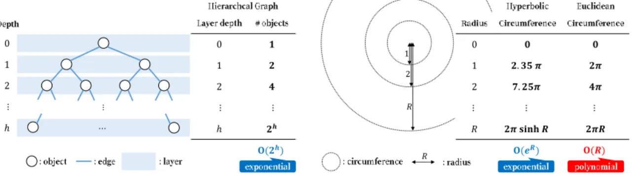
However, current ordinal embedding methods use Euclidean space as a primary choice, mainly due to natural generalization of intuition-friendly and visual three-dimensional space (Ganea et al., 2018a). These methods may not be able to reflect semantic dissimilarities between objects or demand a substantial increases in model complexity and computational cost, especially when data come from hierarchical structure, whereas the hierarchical struc-ture is exhibited in reality by many types of complex data, such as datasets with power-law distributions, in natural language area and scale-free networks (Krioukov et al.,2010;Nickel and Kiela, 2017). Take a hierarchical structure given by a complete balanced binary tree in Figure 1 as an example. The number of objects in each layer grows exponentially with respect to h, which is given by 2h. However, the expanding speed of Euclidean space is polynomial (slower than exponential) as the circumference C(R) of radius R is given by
C(R) = 2πsinhR ≈ πexpR. This motivates us to seek a feasible non-Euclidean space that expands exponentially so as to achieve effective ordinal embeddings by capturing the hierarchical structure.
Inspired by the above, we focus on sectional curvatureκ, which characterizes the expand-ing speed of a space. Accordexpand-ing to Bertrand-Diguet-Puiseux theorem, which claims that
C(R) = 2π(R−16κR3) +O(R4) asR→+0, achieving faster expanding speed than
polyno-mial requires lower curvature, i.e., negative curvature. On the other hand, in essence there is no constant negative curvature space other than hyperbolic (Killing-Hopf theorem e.g., in (Lee,2006)). Fortunately, the hyperbolic space of two dimension or higher has exponential expanding speed. Specifically, in the 2-dimensional hyperbolic space the circumference is given byC(R) = 2πsinhR≈πexpR. Such exponential expanding speed explicitly matches hierarchical structure, as shown in Figure 1. Moreover, Sarkar(2011) has theoretically ex-plained that given an arbitrary tree, we have embeddings of its vertices with arbitrary small distance distortion in the 2-dimensional hyperbolic space. These facts demonstrate hierarchy-friendly property of hyperbolic space in low-dimensional setting, which satisfies our motivation. This preferable property of hyperbolic space in embedding has been sup-ported by recent success of hyperbolic space in many embedding settings and applications such as graph embedding (Shavitt and Tankel, 2008;Nickel and Kiela,2017), embedding from graph Laplacian (Alanis-Lobato et al.,2016), metric multi-dimensional scaling (Sala et al., 2018), Internet graph embedding (Shavitt and Tankel, 2008), and visualization of large taxonomies (Nickel and Kiela,2017).
In this paper, we are the first to apply hyperbolic space into ordinal embedding and propose a novel hyperbolic ordinal embedding (HOE) model to capture hierarchical struc-ture and preserve ordinal relations simultaneously. Furthermore, we prove the suitability
of hyperbolic space and limitations of Euclidean space for ordinal relation with hierarchical structure in theory.
We summarize our main contributions as follows:
• A hyperbolic ordinal embedding (HOE) is proposed to embed hierarchical structure data in an extremely low-dimensional hyperbolic space. We reformulate the ordinal embedding problem into a general metric space setting with hyperbolic space setting as a special case, and then propose two simple yet effective continuous loss functions for probabilistic-model-based and margin-loss-based models, respectively.
• We give theoretical analyses to clarify advantages of using hyperbolic space against Euclidean approach (in Section 6) in terms of ordinal embedding for hierarchical structural data: (1) for Euclidean space of any dimension, there exist ordinal relations that cannot be preserved in embeddings; (2) the use of hyperbolic space can achieve effective embedding with ordinal relations preserved in a space of extremely low (e.g.,2) dimensionality.
• Experiments on both artificial and real datasets have demonstrated that the proposed method outperforms existing Euclidean-space-based baselines for embedding hierar-chical structure data in a significantly low-dimensional (e.g., 2, 4, 8, 16) space.
⋯ ⋮ 0 𝟏 1 𝟐 2 𝟒 ⋮ ⋮ ℎ 𝟐𝒉 𝐎(𝟐𝒉) 0 𝟎 𝟎 1 𝟐. 𝟑𝟓 𝝅 𝟐𝝅 2 𝟕. 𝟐𝟓𝝅 𝟒𝝅 ⋮ ⋮ ⋮ 𝑅 𝟐𝝅 𝐬𝐢𝐧𝐡 𝑹 𝟐𝝅𝑹 𝐎(𝒆𝑹) 𝐎(𝑹) 𝑅 2 1 0 1 2 ⋮ ℎ 𝑅
Figure 1: Exponential growth of objects in a hierarchical data and space expansion speed of hyperbolic and Euclidean space.
2. Related Work
Various ordinal embedding approaches have been proposed. Under probabilistic-model-based setting, CLK (Tamuz et al.,2011) was proposed to reduce the complexity of obtain-ing high quality approximations of similarity triplets via an information theoretic adaptive sampling approach. Considering that using similarity triplets is insufficient for obtain-ing a truthful embeddobtain-ing of objects, t-STE (Van Der Maaten and Weinberger, 2012) was then proposed to collapse similar points and repel dissimilar points in the embedding with-out resulting in additional constraint violations. Under margin-loss-based setting, G-NMD (Agarwal et al., 2007) aimed to embed data when ordinal relations can be contradictory
and need not be specified for all pairs of dissimilarities. Regarding that the similarities of objects may not be mutually consistent according to different tasks, McFee and Lanck-riet (2011) integrated heterogeneous data so as to optimally conform to measurements of perceptual similarity. Later, LOE (Terada and Luxburg, 2014) was proposed to achieve embedding that not only preserves the ordinal constraints, but also the density structure of dataset. Though the effectiveness of existing ordinal embeddings has been demonstrated, none of them pay attention to the compatibility of embedding space and achieve embedding in hyperbolic space.
Recently, hyperbolic space has been extensively studied in many research areas ( Alanis-Lobato et al., 2016; Nickel and Kiela, 2017; Sala et al., 2018). For example, Shavitt and Tankel (2008) embeded Internet data in hyperbolic space, since Internet structure has a highly connected core and long stretched tendrils, where most of the routing paths between nodes in the tendrils pass through the core. To enhance the efficiency of embedding of big networks,Alanis-Lobato et al.(2016) then used a Laplacian-based model for geometric analysis of big networks. Poincar´e Embedding (Nickel and Kiela,2017) aimed at learning representations of symbolic data so that it simultaneously learns the similarity and the hierarchy of objects. Later, Ganea et al. (2018b) bridged the gap between hyperbolic and Euclidean geometry in the context of neural networks and deep learning by generalizing deep neural models to the Poincar´e model of the hyperbolic geometry. Balancing the trade-off between precision and dimensionality of embedding, H-MDS (Sala et al., 2018) was proposed as a general approach that can embed trees into hyperbolic space with arbitrarily low distortion. Although these approaches can achieve effective embedding by capturing hierarchy structure with hyperbolic space, the ordinal relations which often naturally exist among data cannot be utilized by them.
3. Hyperbolic Geometry
In this section, we introduce basic notations and then briefly review hyperbolic geometry with its real coordinate space representation.
Notations LetR,R≥0,Z, andZ>0 denote the real number set, non-negative real number
set, integer set, and positive integer set, respectively. We denoteD-dimensional real coordi-nate space and D×D0 real matrix space byRD and RD×D
0
, respectively. We let 0D ∈RD
and ID ∈RD×D denote the D-dimensional zero vector andD-dimensional identity matrix,
respectively. sgn :R→ {−1,0,1} denotes the sign function defined by
sgn(x) := −1 x <0 0 x= 0 +1 x >0 . (2)
ForN ∈Z>0, we denote the set {1,2, . . . , N}by [N].
Hyperbolic Geometry in Coordinate Space Since there is unique hyperbolic space up to similarity if the dimension is fixed, in the following, we fix the sectional curvature of hyperbolic space to be -1, that is,κ=−1 for simplicity of discussion. For hyperbolic space, there exist several models, i.e., representation ways in real coordinate space, such as the
hyperboloid model, Klein disk model, Poincar´e disk model and Poincar´e upper plain model. As these models are isometric to one another, the discussion on the distance structure of hyperbolic space in one model is equivalent to that in another model. In the following, we explain hyperbolic space using the hyperboloid model. TheD-dimensional hyperbolic space
HD is a metric space
HD, dHD
, whereHD and dHD :HD×HD →R≥0 are defined by HD := n x∈RD+1 x >G Mx=−1, x0 >0 o dHD(x,y) := arcosh −x>GMy , (3)
where arcosh denotes the area hyperbolic cosine function (the inverse function of the hy-perbolic cosine function), and GM denotes
GM:= −1 0>D 0D ID ∈R(D+1)×(D+1). (4)
4. Euclidean Ordinal Embedding
We consider embedding problem of N ∈Z>0 objects. In the following, we identify the N
objects with the integer set [N]. Let the sequenceS = (((is, js),(ks, ls)), ys)Ss=1be an ordinal
data set, in whichis, js, ks, ls∈[N] and ys∈ {−1,+1} fors= 1,2, . . . , S. Here, ifys=−1, isand js are more similar to each other thanksand lsi.e., the dissimilarity betweenis and js are larger than that between ks and ls, and otherwise if ys = +1. An ordinal data set S = (((is, js),(ks, ls)), ys)Ss=1 is called ordinal triplet set ifis=ks is satisfied for alls∈[S].
The D-dimensional Euclidean space denoted by RD is a metric space
RD, dRD , where dRD :RD×RD →R≥0 is given by dRD(x,y) := p (x−y)>(x−y).
Existing ordinal embedding using the D-dimensional Euclidean space RD is to obtain
embedding xn∈RD forn∈[N] such that
sgn(dRD(xis, xjs)−d
RD(xks, xls)) =ys (5)
is satisfied for as manys∈[S] as possible.
Denote the Probabilistic-model-based Ordinal Embedding and the Margin-loss-based
Ordinal Embedding as POE and MOE, respectively. In both Euclidean POE and MOE, the loss function of (xn)n∈[N]on ordinal data S = (((is, js),(ks, ls)), ys)Ss=1 is given by
LS; (xn)n∈[N] := 1 S X s∈[S] ` ((is, js),(ks, ls), ys); (xn)n∈[N] , (6)
with their own specific one point loss function ` of (xn)n∈[N] on one point ordinal datum
(((i, j),(k, l)), y).
• Euclidean POE (EPOE) For the object quadruple ((i, j),(k, l)), the probability of
y = −1 is high if the distance dX(xi, xj) is shorter than dX(xk, xl) and the probability of y = +1 is high otherwise. The dependency of the distribution of y on the distances is
defined by a decreasing function f :R≥0→R≥0. Then, we have the following probabilistic model. Pry|((i, j),(k, l)); (xn)n∈[N] := f(dRD(xi, xj)) f(dRD(xi, xj)) +f(d RD(xk, xl)) y=−1 f(dRD(xk, xl)) f(dRD(xi, xj)) +f(d RD(xk, xl)) y= +1 (7)
We callf a kernel function. The loss function`prb of (xn)n∈[N]on one point ordinal datum
(((i, j),(k, l)), y) is given by `prb (((i, j),(k, l)), y); (xn)n∈[N] :=−log Pr y|((i, j),(k, l)); (x)n∈[N] . (8) Then, the loss function in EPOE of (xn)n∈[N]on ordinal dataS = (((is, js),(ks, ls)), ys)Ss=1
is derived by substituting `=`prb to (6). Take one of the most representative approaches,
stochastic triplet embedding (Van Der Maaten and Weinberger,2012), as an example. The probabilistic model given by (7) is reduced to that of the stochastic triplet embedding and t-distributed stochastic triplet embedding in (Van Der Maaten and Weinberger,2012) with the Gaussian kernelf(d) = exp −d2
and Student’s t-distribution kernelf(d) =1 +dα2α, respectively. Note that in (Van Der Maaten and Weinberger,2012), only are ordinal triplet data cases considered, while we above generalized it into general ordinal data cases.
• Euclidean MOE (EMOE) We define a soft margin loss for this approach (Agarwal et al., 2007; Terada and Luxburg, 2014). The soft margin loss function `mgn of (xn)n∈[N]
on one point ordinal datum (((i, j),(k, l)), y) is given by
`mgn (((i, j),(k, l)), y); (xn)n∈[N] := [δ−(dRD(xis, xjs)−d RD(xks, xls))·ys]+ q , (9) whereδ∈R≥0 is a margin hyperparameter andq∈R≥0 is a power index which adjusts the
loss. Then, the loss function in EMOE of (xn)n∈[N]on ordinal dataS = (((is, js),(ks, ls)), ys)Ss=1
is derived by substituting`=`mgn to (6). The loss function in (9) is reduced to that of the
soft margin model in (Terada and Luxburg,2014) ifq = 2, and is indirectly reduced to the loss function in (Agarwal et al.,2007) if q = 1, whereas they obtain the distance matrix in
RD withD=N in (Agarwal et al.,2007), instead of directly obtaining embeddings inRD.
5. Hyperbolic Ordinal Embedding
Our motivation is ordinal embedding in hyperbolic space. The key idea is to generalize existing methods into those in general metric spaces and obtain our hyperbolic ordinal embedding as a special case.
5.1. General Ordinal Embedding
In this section, we obtain ordinal embedding in a general metric space X = (X, dX), where
5.1.1. Problem Settings
Sharing the same motivation as the Euclidean case, the objective of embedding objects [N] in metric space X is to obtain embeddingxn∈Xfor n∈[N] such that
sgn(dX(xis, xjs)−dX(xks, xls)) =ys (10) is satisfied for as many s∈[S] as possible. Therefore, the ordinal embedding is formulated as minimizing the classification loss function, as defined below.
Definition 1 (Classification Loss Function) Let [N] be objects and (xn)n∈[N] be their
embeddings. The classification loss function of(xn)n∈[N]on ordinal datum(((i, j),(k, l)), y),
in which i, j, k, l∈[N]and y∈ {±1}, is defined by
`cls (((i, j),(k, l)), y); (xn)n∈[N] := ( 0 sgn(dX(xis, xjs)−dX(xks, xls)) =ys 1 sgn(dX(xis, xjs)−dX(xks, xls))6=ys (11)
The classification loss function of embedding(xn)n∈[N]on ordinal dataS = (((is, js),(ks, ls)), ys)Ss=1,
in which is, js, ks, ls∈[N]and ys∈ {±1} for alls∈[N], is defined by LclsS; (xn)n∈[N] := 1 S X s∈S `cls (((is, js),(ks, ls)), y); (xn)n∈[N] . (12)
The embedding (xn)n∈[N] is called non-contradictory to S if Lcls
S; (xn)n∈[N]
= 0.
5.1.2. Loss Functions
The loss function in Definition 1 is a hard classification loss and not easy to optimize due to the discontinuity of the sign function. We first consider general idea for relaxation of the original loss function, and then introduce a probabilistic model and sort margin based loss function for specific loss functions. The ideal conditions of the loss function are listed as follows:
• The loss function should be continuous with respect to the embeddings (xn)n∈[N]. • For ordinal data (((i, j),(k, l)),−1) inS, the loss function should be decreasing with
respect to the distance dX(xi, xj) and increasing with respect to dX(xk, xl), and vice versa for (((i, j),(k, l)),+1).
Therefore, we consider the loss functionL in the following form
LS; (xn)n∈[N] := 1 S X s∈[S] `((is, js),(ks, ls), ys); (xn)n∈[N] , (13)
with one datum loss function` given by
`
((i, j),(k, l), y); (xn)n∈[N]
:=g(dX(xi, xj), dX(xk, xl);y), (14) whereg:R≥0×R≥0× {±1},(d, d0, y)7→g(d, d0;y) satisfies the following:
• g(d, d0;−1) is decreasing with respect todand increasing with respect to d0.
• g(d, d0; +1) is increasing with respect todand decreasing with respect to d0.
This general idea allows us to apply in hyperbolic space analogical ideas to EPOE and EMOE. As a result, we obtain specific loss functions, GPOE and GMOE, as shown below.
• General POE (GPOE) One way to avoid the discontinuous loss function is to intro-duce a probabilistic model, as in EPOE. We design a conditional probability distribution model ofy, as follows: Pr y|((i, j),(k, l)); (xn)n∈[N] := f(dX(xi, xj)) f(dX(xi, xj)) +f(dX(xk, xl)) y=−1 f(dX(xk, xl)) f(dX(xi, xj)) +f(dX(xk, xl)) y= +1 , (15)
wheref :R≥0 →R≥0 is a kernel function. By the above probabilistic model, one point loss
function in GPOE `prb of (xn)n∈[N] on one point ordinal datum (((i, j),(k, l)), y) is given
by `prb (((i, j),(k, l)), y); (xn)n∈[N] :=−log Pr y|((i, j),(k, l)); (x)n∈[N] . (16) Then, the loss function in GPOE of (xn)n∈[N] on ordinal dataS = (((is, js),(ks, ls)), ys)Ss=1
is derived by substituting `=`prb to (13). When X is the D-dimensional Euclidean space RD, GPOE is reduced to EPOE.
• General MOE (GMOE) Another way to avoid the discontinuous loss function is to replace it by a soft loss function, as in EMOE. We define a soft margin loss as follows. The one point soft margin loss function `mgn of (xn)n∈[N] on one point ordinal datum
(((i, j),(k, l)), y) is given by `mgn (((i, j),(k, l)), y); (xn)n∈[N] := [δ−(dX(xis, xjs)−dX(xks, xls))·ys]+ q , (17) whereδ∈R≥0 is a margin hyperparameter andq∈R≥0 is a power index which adjusts the
loss. Then, the loss function in GMOE of (xn)n∈[N]on ordinal dataS= (((is, js),(ks, ls)), ys)Ss=1
is derived by substituting `=`mgn to (13). WhenX is theD-dimensional Euclidean space RD, GMOE is reduced to EMOE.
5.2. Hyperbolic Ordinal Embedding
With the generalization in Section 5.1.2, Hyperbolic POE and MOE can be obtained by substitutingX=HD to (15) and (17), respectively, wherex1,x2, . . . ,xN ∈HD.
•Hyperbolic POE (HPOE) The probabilistic model of HPOE using theD-dimensional hyperbolic space HD is derived by substituting
X=HD to (15) as follows: Pry|((i, j),(k, l)); (xn)n∈[N] := f(dHD(xi,xj)) f(dHD(xi,xj)) +f(d HD(xk,xl)) y =−1 f(dHD(xk,xl)) f(dHD(xi,xj)) +f(d HD(xk,xl)) y = +1 . (18)
• Hyperbolic MOE (HMOE) The one point loss function of HMOE using the D -dimensional hyperbolic space HD is derived by substituting
X=HD to (17) as follows: `mgn (((i, j),(k, l)), y); (xn)n∈[N] := [δ−(dHD(xis,xjs)−d HD(xks,xls))·ys]+ q . (19) Here, as in (17),δ ∈R≥0 is a margin hyperparameter and q∈R≥0 is a power index which
adjusts the loss.
5.3. Optimization
Similar to (Van Der Maaten and Weinberger, 2012), the stochastic gradient method is applied to optimize (13). Note that the following optimization method can be applied to the loss function of HPOE and HMOE, because the loss functions of these methods are special cases of that in (13). We uniformly at random choose a subsequence B of [S] and substitute Bfor [S], then we have stochastic loss of the loss in (13) as follows:
˜ LS; (xn)n∈[N] := 1 |B| X s∈B ` (((is, js); (ks, ls)), y),(xn)n∈[N] , (20)
where |B| denotes the number of elements in B. Then, we use the gradient of (20) as a stochastic gradient of the loss function in (13) and then optimize the loss function in (13) by stochastic Riemannian sub gradient method (Zhang and Sra,2016). The update rule is given by xn←expxn πxn G−xn1 ∂ ∂xn ˜ L , (21)
whereGxn denotes the metric matrix onxn,πx denotes the projection to the tangent space onxn, and expxdenotes the exponential map onxn. In theD-dimensional hyperbolic space, the formulae for these operations appear in e.g., (Nickel and Kiela,2018) as follows.
Gx =GM (in (4)), πx v0 =v0+x>GMx x, expx(v) = coshpv>GMv x+ sinhcpv>GMv v, (22)
where sinhc denotes the hyperbolic sine cardinal function, which is given by
sinhcx= (
sinhx
x x6= 0
1 x= 0 . (23)
Using these formulae, we can optimize the loss function of HPOE and HMOE. Note that we can also apply the above optimization method in the Poincar´e disk model of hyperbolic space by the formulae that appears in e.g., (Ganea et al., 2018a), although the result is isometric to the formulae for the hyperboloid model in this section.
6. Hyperbolic vs. Euclidean
In this section, we discuss the theoretical advantages of using hyperbolic space against using Euclidean space. Our interest is the situation in which the ordinal data comes from ground-truth hierarchical structure. For formal discussion, we define such a situation as the case when we have graphical ordinal data of a graph that is a tree, which intuitively gives a hierarchical structure as in Figure 1. In this section, after defining graphical ordinal data as a preliminary, we discuss hyperbolic and Euclidean space cases.
Preliminary: Graphical Ordinal Data
Definition 2 Let G = ([N],E) be an undirected graph with vertex set [N] and edge set E. We denote the graph distance function by dG. A sequence S = (((is, js),(ks, ls)), ys)Ss=1 is
called graphical ordinal data (GOD)of G when
sgn(dG(is, js)−dG(ks, ls)) =ys (24)
is satisfied for all s∈ [S]. GOD are called graphical ordinal triplet data (GOTD) of G if
is=ks is satisfied for alls∈[S], and GOD are called completeif for all pairs((i, j),(k, l))
of vertex pair such that dG(i, j)−dG(k, l) 6= 0, there exists s ∈ [S] such that either of the following is satisfied.
• ((is, js),(ks, ls)) = ((i, j),(k, l))and ys= sgn(dG(is, js)−dG(ks, ls)) • ((is, js),(ks, ls)) = ((k, l),(i, j))and ys= sgn(dG(ks, ls)−dG(is, js))
GOTD are called complete if the condition above is satisfied for all pairs ((i, j),(k, l)) of vertex pair such that i=k and dG(i, j)−dG(k, l)6= 0.
We are interested in the case whereG is a tree, which corresponds to a typical hierarchical structure. We consider both the complete GOD case and complete GOTD case. Note that, as the complete GOTD are a subset of the complete GOD, to find embedding that is contradictory to the complete GOTD are easier than to find embedding that is non-contradictory to the complete GOD.
Hyperbolic Space Case As shown in the following theorem, there is a non-contradictory embedding in HD to complete GOD of a tree, even inD= 2.
Theorem 3 For any tree G and GOD S of G, there exists an embedding (xn)n∈[N] in H2
that is non-contradictory to G.
Corollary 4 For any tree G and GOTDS ofG, there exists an embedding(xn)n∈[N] inH2
that is non-contradictory to G.
Theorem 3 is obtained from the result in Sarkar (2011), and it also gives a concrete con-struction of the embedding. The complete proof of Theorem 3 is given in Supplementary Materials. Corollary4follows Theorem3, because the complete GOTD are included in the complete GOD.
Remark 5 As the D-dimensional hyperbolic space HD (D ≥ 2) includes 2-dimensional
Euclidean Space Case Contrary to hyperbolic space, there is no non-contradictory embedding inRDto complete GOTD of some trees. Before we show the results, we introduce
some definitions.
Definition 6 Let G = ([N],E) be an undirected graph with vertex set [N] and edge set
E. The degree deg (v) of v ∈ [N] is defined by deg (v) := |{u∈[N]| (u, v)∈ E}|. We denote the maximum degree of any vertex in G by deg (G), which is defined by deg (G) := max{deg(v) | v∈[N]}.
Definition 7 Let the D-dimensional sphere and the distance function on it be denoted by SD and dSD, respectively, which are given by
SD := n x∈R(D+1) x > x= 1 o , dSD(x,y) := arccos x>y . (25)
The π3 packing number M SD, dSD,π3
of SD, dSD
is the maximal number of points that can be π3-separated, which is defined by
MSD, dSD, π 3 := maxnN ∈Z≥0 ∃x1,x2, . . . ,xN ∈S D,∀i, j ∈[N], d SD(xi,xj)> π 3 o . (26) Note that the packing number M SD, dSD,π3
is finite for all D ∈ Z>0 and monotonous
increasing function with respect to D, because for anyD, D0 ∈Z>0 such that D < D0,SD
is a subspace of SD
0
. The following theorem clarifies the limitation of Euclidean space in ordinal embedding setting.
Theorem 8 For any dimensionality D, for all graph G that is tree, if deg (G) is larger than M SD−1, dSD−1,π
3
, then no embedding (xn)n∈[N] in RD is non-contradictory to the
complete GOTD of G.
Corollary 9 For any dimensionality D, for all graph G that is tree, if deg (G) is larger than M SD−1, dSD−1,π3
, then no embedding (xn)n∈[N] in RD is non-contradictory to the complete GOD of G.
The proof of Theorem8is given in Supplementary Materials. Corollary9follows Theorem8, because the complete GOTD are included in the complete GOD.
Remark 10 Theorem8 and Corollary 9 give a limitation of Euclidean space in embedding GOD of a tree. According to Theorem3,8, and Corollary4,9, two dimension is high enough in hyperbolic space for embedding of GOD of tree, but not all tree graphs can be embedded even in higher-dimensional Euclidean space. Hence, we can conclude that hyperbolic space is more suitable than Euclidean space for embedding of hierarchical ordinal data.
Remark 11 (Technical contribution of Theorem 8) Although the advantage of hyper-bolic space against Euclidean space for embedding trees has shown in graph embedding set-tings (e.g., Sarkar (2011)), the limitation of Euclidean space in embedding from ordinal triplet data given by Theorem 8 has not been clarified. Theorem 8 is not trivially derived from the graph embedding setting’s results, because the requirements in the triplet ordinal
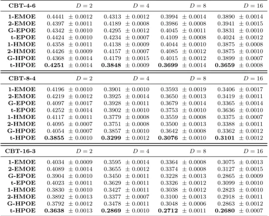
Table 1: Classification errors (mean± standard error) in artificial datasets. CBT-4-6 D= 2 D= 4 D= 8 D= 16 1-EMOE 0.4441 ±0.0012 0.4313 ±0.0012 0.3994 ±0.0014 0.3890 ±0.0014 2-EMOE 0.4397 ±0.0011 0.4189 ±0.0008 0.3986 ±0.0008 0.3941 ±0.0015 G-EPOE 0.4342 ±0.0010 0.4295 ±0.0012 0.4045 ±0.0011 0.3831 ±0.0010 t-EPOE 0.4424 ±0.0010 0.4234 ±0.0007 0.4109 ±0.0008 0.4024 ±0.0012 1-HMOE 0.4358 ±0.0011 0.4138 ±0.0009 0.4044 ±0.0010 0.3875 ±0.0008 2-HMOE 0.4426 ±0.0009 0.4157 ±0.0007 0.4085 ±0.0012 0.3875 ±0.0010 G-HPOE 0.4368 ±0.0014 0.4179 ±0.0015 0.4015 ±0.0012 0.3899 ±0.0007 t-HPOE 0.4251 ±0.0014 0.3848 ±0.0009 0.3699 ±0.0014 0.3659 ±0.0008 CBT-8-4 D= 2 D= 4 D= 8 D= 16 1-EMOE 0.4196 ±0.0010 0.3901 ±0.0010 0.3593 ±0.0019 0.3406 ±0.0017 2-EMOE 0.4219 ±0.0012 0.3925 ±0.0014 0.3650 ±0.0013 0.3419 ±0.0011 G-EPOE 0.4097 ±0.0017 0.3928 ±0.0011 0.3679 ±0.0014 0.3365 ±0.0014 t-EPOE 0.4252 ±0.0014 0.3902 ±0.0010 0.3753 ±0.0010 0.3636 ±0.0010 1-HMOE 0.4117 ±0.0011 0.3779 ±0.0008 0.3559 ±0.0008 0.3375 ±0.0007 2-HMOE 0.4095 ±0.0007 0.3751 ±0.0008 0.3500 ±0.0013 0.3388 ±0.0011 G-HPOE 0.4054 ±0.0007 0.3857 ±0.0010 0.3642 ±0.0008 0.3362 ±0.0012 t-HPOE 0.3855 ±0.0010 0.3299 ±0.0012 0.3076 ±0.0010 0.3101 ±0.0012 CBT-16-3 D= 2 D= 4 D= 8 D= 16 1-EMOE 0.4034 ±0.0009 0.3595 ±0.0014 0.3364 ±0.0008 0.3075 ±0.0013 2-EMOE 0.4089 ±0.0014 0.3655 ±0.0012 0.3374 ±0.0008 0.3127 ±0.0015 G-EPOE 0.3904 ±0.0010 0.3450 ±0.0011 0.3228 ±0.0013 0.2865 ±0.0009 t-EPOE 0.4023 ±0.0011 0.3629 ±0.0011 0.3326 ±0.0012 0.3099 ±0.0010 1-HMOE 0.3830 ±0.0010 0.3427 ±0.0011 0.3038 ±0.0012 0.2823 ±0.0010 2-HMOE 0.3892 ±0.0013 0.3377 ±0.0007 0.3100 ±0.0013 0.2918 ±0.0011 G-HPOE 0.3792 ±0.0012 0.3478 ±0.0011 0.3048 ±0.0006 0.2863 ±0.0012 t-HPOE 0.3638 ±0.0013 0.2869 ±0.0010 0.2712 ±0.0011 0.2680 ±0.0007
data setting is weaker than the graph embedding setting. Specifically, the triplet ordinal data setting only cares the distance comparison in triplets, in which i=k, while the graph embedding setting cares uniform distortion, which corresponds to distance comparison in quadruplets, where i 6= k is possible. Theorem 8 shows that Euclidean space cannot sat-isfy even the requirements of the ordinal triplet data setting, which is easier than the graph embedding setting.
7. Experiments
7.1. Experimental Settings
Methods To demonstrate the effectiveness of using hyperbolic space, we use the following Euclidean-space-based methods as baselines.
q-EMOEThe loss function is given by`mgn in (9) with power indexq, whereX=RD. In
the experiments, we used q= 1,2.
f-EPOEThe loss function is given by `prb in (8) with kernel functionf, whereX=RD.
In this experiment, EPOE with the Gaussian kernel f(d) = exp −d2
and Student’s t-distribution kernel f(d) =
1 +dα2
α
are used, which we call G-EPOE (Gaussian EPOE) and t-EPOE (t-distributed EPOE).
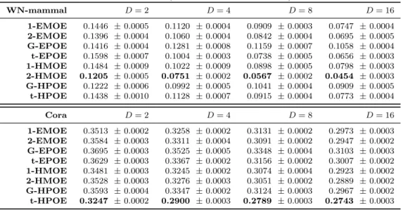
Table 2: Classification errors (mean ±standard error) in real datasets. WN-mammal D= 2 D= 4 D= 8 D= 16 1-EMOE 0.1446 ±0.0005 0.1120 ±0.0004 0.0909 ±0.0003 0.0747 ±0.0004 2-EMOE 0.1396 ±0.0004 0.1060 ±0.0004 0.0842 ±0.0004 0.0695 ±0.0005 G-EPOE 0.1416 ±0.0004 0.1281 ±0.0008 0.1159 ±0.0007 0.1058 ±0.0004 t-EPOE 0.1598 ±0.0007 0.1004 ±0.0003 0.0738 ±0.0005 0.0656 ±0.0003 1-HMOE 0.1484 ±0.0009 0.1022 ±0.0009 0.0898 ±0.0005 0.0798 ±0.0003 2-HMOE 0.1205 ±0.0005 0.0751 ±0.0002 0.0567 ±0.0002 0.0454 ±0.0003 G-HPOE 0.1222 ±0.0006 0.0992 ±0.0005 0.1041 ±0.0004 0.0909 ±0.0005 t-HPOE 0.1438 ±0.0010 0.1128 ±0.0007 0.0915 ±0.0004 0.0773 ±0.0004 Cora D= 2 D= 4 D= 8 D= 16 1-EMOE 0.3513 ±0.0002 0.3258 ±0.0002 0.3131 ±0.0002 0.2973 ±0.0003 2-EMOE 0.3584 ±0.0003 0.3311 ±0.0004 0.3091 ±0.0002 0.2947 ±0.0002 G-EPOE 0.3695 ±0.0003 0.3525 ±0.0005 0.3348 ±0.0004 0.3103 ±0.0003 t-EPOE 0.3629 ±0.0003 0.3367 ±0.0002 0.3156 ±0.0002 0.3007 ±0.0002 1-HMOE 0.3481 ±0.0003 0.3245 ±0.0002 0.3074 ±0.0004 0.2923 ±0.0002 2-HMOE 0.3528 ±0.0003 0.3276 ±0.0003 0.3051 ±0.0002 0.2889 ±0.0002 G-HPOE 0.3593 ±0.0004 0.3347 ±0.0002 0.3124 ±0.0003 0.2967 ±0.0002 t-HPOE 0.3247 ±0.0002 0.2900 ±0.0003 0.2789 ±0.0003 0.2743 ±0.0003
For the proposed hyperbolic methods, we use the following methods:
q-HMOE The loss function is given by `mgn with power index q, where X=HD. In the
experiments,q= 1,2.
f-HPOEThe loss function is given by`prbin (16) with kernel functionf, whereX=HD.
Similar to G-EPOE and t-EPOE, we use the same Gaussian kernel and Student’s t-distrubution kernel for HPOE, and name them G-HPOE and t-HPOE, respectively.
Evaluation Protocol We conducted experiments on ordinal triplet data sets and ran each method 10 times to report their average classification errors along with standard errors. We created GOTD of ground-truth graph and randomly split the data set into training data, validation data, and test data. We trained each method on the training data, and selected a hyperparameter that gives the lowest classification error in grid-search on validation data as the best hyperparameter.
Optimization For optimization of all the methods, the stochastic Riemannian sub gra-dient method (Zhang and Sra, 2016) was applied. Note that this optimization method is reduced to the vanilla stochastic gradient descent method for the baselines, in which Eu-clidean space is used. The specific algorithm for our hyperbolic methods is given in Section
5.3. For all the methods, the constant learning rate was selected by grid-search.
Parameter Settings The batch size and the number of epoch in stochastic gradient descent are both fixed to 1000. In margin-loss-based methods, the margin hyperparameter
δ is fixed to 1.0. The learning rate was selected from {0.1,1.0,10.0} by grid-search. We report the results inD= 2,4,8,16.
7.2. Experiments on Artificial Datasets
To validate the effectiveness of embedding in hyperbolic space, we constructed a typical hierarchical structure dataset, i.e., complete balanced tree (CBT).
Datasets CBTDenoting them-nary complete balanced tree with the depthhby
CBT-m-h, we use CBT-4-6, CBT-8-4 and CBT-16-3 for the experiments. Note that the number of the leaves of which are all 4096. We randomly selected 10000, 1000, and 1000 triplets for training, validation, and test, respectively in the experiments.
Results Table 1 shows that t-HPOE achieves the best result in all cases, which vali-date the effectiveness of using hyperbolic space. Moreover, both q-HMOE and f-HPOE
performs better than the corresponding Euclidean methods in most cases. Taken D = 2 as an example, t-HPOE achieves the lowest errors with 0.4281 in CBT-4-6, as well as 0.3855 and 0.3638 in CBT-8-4 and CBT-16-3, respectively. However, as the best per-former among Euclidean methods, G-EPOE obtains the 0.4342, 0.4097, and 0.3904 only. This is because the expanding speed of hyperbolic space matches hierarchical structure of data, so that better embeddings can be achieved in very low dimensionality. Taking it a step further, we find that t-HPOE outperforms G-EPOE with a larger margin with lower dimensionality of space, such as 0.2865 when D = 2 and 0.0185 when D = 16 for
CBT-16-3 dataset. It is also interesting to note that superiority of t-HPOE decreases with increasingm. For example,t-HPOEachieves low errors thanG-EPOEwith 0.0061 in CBT-4-6 and 0.0266 in CBT-16-3 when D = 2. These phenomena are in line with theoretical analyses in Corollary 4and Theorem 8.
7.3. Experiments on Real Datasets
We also compared the proposed methods to Euclidean-space-based methods on two real datasets that are of hierarchy.
Datasets WN-mammal(Nickel and Kiela,2017) is a subset in WordNet1, which consists of more than 900 hyponyms ofmammal. This dataset owns hierarchical structure, because a hypernym often related to many hyponyms. Cora(ˇSubelj and Bajec, 2013) is a author citation dataset (McCallum et al.,2000) that contains more than 20000 computer science papers collected from web as vertices of graph. The references are parsed automatically and regarded as edges. Since reputable papers always are cited by many other papers, there should exist an underlying hierarchical structure.
The graph of each dataset is ground-truth and we derived triplets, i.e., GOTD (in Definition 2), from these graphs. Following (Liu et al., 2017), to avoid overfitting, we randomly selected 30000 triplets for training in WM-mammal, as well as 3000 triplets for validation and test each. Since Cora has a larger number of objects, we used more triplets, i.e., 100000, 10000, and 10000 for training, validation, and test, respectively.
Results The classification errors of hyperbolic methods against Euclidean baselines are given in Table 2 We can see that when D = 2, 2-HMOE shows the lowest mean error 0.1205 in WN-mammal and t-HPOE shows the lowest error 0.3247 in Cora, whereas the best results of Euclidean methods are 0.1396 and 0.3513 only. This again demonstrates the effectiveness of the proposed hyperbolic methods for embedding hierarchical strurctural data in a low-dimensional space.
8. Conclusion
In this paper, we have proposed a novel hyperbolic ordinal embedding (HOE) method to embed data that are of hierarchical structure in hyperbolic space. Due to the hierarchy-friendly property of hyperbolic space, HOE has effectively achieved embedding by capturing the hierarchy and preserving ordinal relations in an extremely low-dimensional space. By using stochastic optimization method, HOE is also of high efficiency. Both theoretical and experimental results have demonstrated the outperformance of HOE over Euclidean methods.
Acknowledgments
This work was supported by JSPS KAKENHI Grant Number JP 18J12201 and 19H01114, and JST-AIP Grant Number JPMJCR19U4.
References
Sameer Agarwal, Josh Wills, Lawrence Cayton, Gert Lanckriet, David Kriegman, and Serge Belongie. Generalized non-metric multidimensional scaling. InArtificial Intelligence and Statistics, pages 11–18, 2007.
Gregorio Alanis-Lobato, Pablo Mier, and Miguel A Andrade-Navarro. Efficient embedding of complex networks to hyperbolic space via their laplacian. Scientific reports, 6:30108, 2016.
Octavian-Eugen Ganea, Gary B´ecigneul, and Thomas Hofmann. Hyperbolic entailment cones for learning hierarchical embeddings. In International Conference on Machine Learning, 2018a.
Octavian-Eugen Ganea, Gary B´ecigneul, and Thomas Hofmann. Hyperbolic neural net-works. In Advances in Neural Information Processing Systems, 2018b.
Dmitri Krioukov, Fragkiskos Papadopoulos, Maksim Kitsak, Amin Vahdat, and Mari´an Bogun´a. Hyperbolic geometry of complex networks. Physical Review E, 82(3):036106, 2010.
Joseph B Kruskal. Multidimensional scaling by optimizing goodness of fit to a nonmetric hypothesis. Psychometrika, 29(1):1–27, 1964a.
Joseph B Kruskal. Nonmetric multidimensional scaling: a numerical method. Psychome-trika, 29(2):115–129, 1964b.
John M Lee. Riemannian manifolds: an introduction to curvature, volume 176. Springer Science & Business Media, 2006.
Hong Liu, Rongrong Ji, Yongjian Wu, and Feiyue Huang. Ordinal constrained binary code learning for nearest neighbor search. InAAAI Conference on Artificial Intelligence, 2017. Andrew Kachites McCallum, Kamal Nigam, Jason Rennie, and Kristie Seymore. Automat-ing the construction of internet portals with machine learnAutomat-ing. Information Retrieval, 3 (2):127–163, 2000.
Brian McFee and Gert Lanckriet. Learning multi-modal similarity. Journal of machine learning research, 12(Feb):491–523, 2011.
Maximilian Nickel and Douwe Kiela. Learning continuous hierarchies in the lorentz model of hyperbolic geometry. In International Conference on Machine Learning, 2018.
Maximillian Nickel and Douwe Kiela. Poincar´e embeddings for learning hierarchical rep-resentations. In Advances in Neural Information Processing Systems, pages 6338–6347, 2017.
Frederic Sala, Chris De Sa, Albert Gu, and Christopher Re. Representation tradeoffs for hyperbolic embeddings. In International Conference on Machine Learning, pages 4457– 4466, 2018.
Rik Sarkar. Low distortion delaunay embedding of trees in hyperbolic plane. InInternational Symposium on Graph Drawing, pages 355–366. Springer, 2011.
Yuval Shavitt and Tomer Tankel. Hyperbolic embedding of internet graph for distance estimation and overlay construction. IEEE/ACM Transactions on Networking, 16(1): 25–36, 2008.
Roger N Shepard. The analysis of proximities: multidimensional scaling with an unknown distance function. i. Psychometrika, 27(2):125–140, 1962a.
Roger N Shepard. The analysis of proximities: Multidimensional scaling with an unknown distance function. ii. Psychometrika, 27(3):219–246, 1962b.
Roger N Shepard. Metric structures in ordinal data. Journal of Mathematical Psychology, 3(2):287–315, 1966.
Lovro ˇSubelj and Marko Bajec. Model of complex networks based on citation dynamics. In
International conference on World Wide Web, pages 527–530. ACM, 2013.
Omer Tamuz, Ce Liu, Serge Belongie, Ohad Shamir, and Adam Tauman Kalai. Adaptively learning the crowd kernel. InInternational Conference on Machine Learning, pages 673– 680, 2011.
Yoshikazu Terada and Ulrike Luxburg. Local ordinal embedding. InInternational Confer-ence on Machine Learning, pages 847–855, 2014.
Laurens Van Der Maaten and Kilian Weinberger. Stochastic triplet embedding. In IEEE International Workshop on Machine Learning for Signal Processing, pages 1–6. IEEE, 2012.
Jing Wang, Feng Tian, Weiwei Liu, Xiao Wang, Wenjie Zhang, and Kenji Yamanishi. Ranking preserving nonnegative matrix factorization. In International Joint Conference on Artificial Intelligence, 2018.
Hongyi Zhang and Suvrit Sra. First-order methods for geodesically convex optimization. In Conference on Learning Theory, pages 1617–1638, 2016.