ALGORITHM
A Paper
Submitted to the Graduate Faculty of the
North Dakota State University of Agriculture and Applied Science
By Minakshi Arya
In Partial Fulfillment of the Requirements for the Degree of
MASTER OF SCIENCE
Major Department: Computer Science
May 2019
North Dakota State University
Graduate School
TitleAUTOMATED DETECTION OF ACUTE LEUKEMIA USING K-MEANS CLUSTERING ALGORITHM
By Minakshi Arya
The Supervisory Committee certifies that this disquisition complies with North Dakota State University’s regulations and meets the accepted standards for the degree of
MASTER OF SCIENCE SUPERVISORY COMMITTEE: Dr. Simone Ludwig Chair Dr. Saeed Salem Dr. Maria Alfonseca-Cubero Approved:
May 8, 2019 Dr. Kendall Nygard
leukocytes. Usually, the analysis of blood cells is performed manually by skilled operators, have numerous drawbacks, such as slow analysis, a non-standard accuracy and skill of the operator. Hence many automated systems are using in order to analyze and classify the blood cells. This paper focuses on an automatic system based on image processing algorithms for the
classification of blood cells for detection of Acute Lymphocytic Leukemia (ALL).
Experiments were ran using 20 models with PCA and seven models namely Medium KNN, Coarse KNN, Cosine KNN, Cubic KNN, Weighted KNN, Ensemble Boosted trees and Ensemble Bagged trees had 99.9% accuracy. These models are evaluated based on the prediction speed, training time, confusion matrix and ROC. Of all models, the weighted KNN classifier is best when using PCA.
ACKNOWLEDGEMENTS
First of all, I would like to express my sincere gratitude to my research advisor, Dr. Simone Ludwig at North Dakota State University for trusting me and giving me the opportunity of research in this new area on Image Processing and Machine Learning. I have learned a lot in this whole process. Her indispensable guidance and encouragement during the research and execution of experiments made this paper possible.
Lastly, I wish to thank my spouse and my children for their continuous support, faith, and encouragement throughout my master studies.
DEDICATION
I would like to dedicate this paper to the beginners who are interested in massively growing Image Processing and Machine Learning field.
ABSTRACT ... iii
ACKNOWLEDGEMENTS ... iv
DEDICATION ... v
LIST OF TABLES ... viii
LIST OF FIGURES ... ix LIST OF ABBREVIATIONS ... xi 1. INTRODUCTION ... 1 2. RELATED WORK ... 4 3. EXPERIMENT ARCHITECTURE ... 8 3.1. Data Set ... 8 3.1.1. Dataset ALL_IDB1 ... 8 3.1.2. Dataset ALL_IDB2 ... 9
4. EXPERIMENTS AND RESULTS ... 10
4.1. The Results of the Different Classifiers and Classification Models ... 22
4.2. Evaluation Measures ... 24
4.3. Results ... 24
4.3.1. Results of Segmentation ... 28
4.4. Characteristics of Classifier Types ... 29
4.4.1. Decision Trees ... 30
4.4.2. Support Vector Machines ... 31
4.4.3. Nearest Neighbor Classifiers ... 33
4.4.4. Ensemble Classifiers ... 34
4.5. Results of Classification ... 35
5. CONCLUSION ... 59 REFERENCES ... 61
1: Image Characteristics ... 11
2: Characteristics of Classifier Types ... 29
3: Different Types of Decision Trees Classifiers ... 30
4: Different Types of Support Vector Machines Classifiers ... 31
5: Different Types of Nearest Neighbor Classifiers ... 33
6: Different Types of Ensemble Classifiers ... 34
7: Model, Accuracy and Training Time ... 38
LIST OF FIGURES
Figure Page
1: Mean Ensemble Subspace Discriminant ... 22
2: Scatter Plot Stats ... 23
3: Scatter Plot Stats Fine Tree Model ... 23
4: Original Image ... 24 5: Gray Image ... 25 6: Cluster1 ... 26 7: Cluster 2 ... 27 8: Cluster3 ... 27 9: Blue Nuclei ... 28 10: Support Vectors ... 32 11: Fine Tree ... 37 12: Coarse KNN ... 39 13: Coarse KNN ROC ... 39 14: Cosine KNN ... 40 15: Cosine KNN ROC ... 40 16: Cubic KNN ... 41 17: Cubic KNN ROC ... 41
18: Ensemble Bagged Trees Confusion Matrix ... 42
19: Ensemble Bagged Trees ROC ... 42
20: Ensemble Boosted Trees ... 43
21: KNN Medium Confusion Matrix ... 43
22: KNN Medium ROC ... 44
24: Linear SVM ROC ... 45
25: SVM Medium Gaussian... 45
26: SVM Medium Gaussian ROC ... 46
27: SVM Coarse Gaussian ... 46
28: Weighted KNN ... 47
29: Weighted KNN ROC ... 47
30: Bar Chart Model - Training Time ... 48
31: Bar Chart Model Type and Accuracy ... 48
32: Stacked Plot Accuracy vs Training Time ... 49
33: Stacked Plot Model and Training Time ... 49
34: Stacked Plot Model and Accuracy ... 50
35: Area Plot Accuracy and Training Time ... 50
36: The X Bar Control Chart Accuracy and Prediction Speed ... 51
37: Scatter Plot between Accuracy and Training Time ... 51
38: Histogram Test Data ... 52
39: Histogram Train Data ... 52
40: Histogram L_blue ... 53
41: Contour pixel_label... 53
42: Medium KNN using PCA with ROC ... 55
43: Medium KNN using PCA with Confusion Matrix ... 56
44: Weighted KNN using PCA with ROC ... 56
45: Weighted KNN using PCA with Confusion Matrix ... 57
46: Ensembled Bagged using PCA with ROC ... 57
LIST OF ABBREVIATIONS RBC...Red Blood Cells
WBC ...White Blood Cells
GLCM ...Gray-Level Co-occurrence Matrix ALL ...Acute lymphocytic leukemia DNA ...Deoxyribonucleic acid KNN ...Nearest Neighbor EU ...Euler Number
PCA ...Principal Component Analysis ROC ...Receiver Operating Characteristic NCI ...National Cancer Institute
There are many types of cancer. Cells in any part of the body can become cancerous when cells in the body begin to grow uncontrolled. Leukemia is cancer that starts in blood cells. Leukemia is divided based on whether the leukemia is acute (fast-growing) or chronic (slower growing), and whether it starts with myeloid cells or lymphoid cells.
Acute lymphocytic leukemia (ALL) is a cancer of the blood and bone marrow. Acute lymphocytic leukemia (ALL) is also called acute lymphoblastic leukemia. “Acute” means that leukemia can progress quickly and creates immature blood cells, rather than mature ones and if not treated, would probably be fatal within a few months. "Lymphocytic" means it develops from early (immature) forms of lymphocytes, a type of white blood cell (WBC). Acute lymphocytic leukemia is a common form of cancer in children, and treatments result in a good chance for a cure, whereas in adults, treatment is greatly reduced. However, if left untreated, acute
lymphocytic leukemia is eventually fatal; it will spread to the lymph nodes, spleen, liver, central nervous system, and other organs.
Acute lymphocytic leukemia occurs when a bone marrow cell develops errors in its deoxyribonucleic acid (DNA). The errors tell the cell to continue growing and dividing, while a healthy cell would stop growing and dividing and eventually die. When this happens, blood cell production becomes abnormal. The bone marrow produces immature cells that develop into leukemic white blood cells called lymphoblasts. These abnormal cells are unable to function properly, and they can build up and crowd out healthy cells. It is not clear what causes the DNA mutations that can lead to acute lymphocytic leukemia.
The symptoms of leukemia include fatigue, unexplained fever, abnormal bruising, headaches, excessive bleeding (such as frequent nosebleeds), unintentional weight loss, and frequent infections, to name a few.
There are around 60,000 new cases of leukemia each year in the U.S. and over 24,000 deaths due to leukemia. Leukemia makes up about 3.7% of all new cancer cases. Acute lymphocytic leukemia is the most common type of leukemia in children, but it can also affect adults. In this type of leukemia, immature lymphoid cells grow rapidly in the blood. It affects almost 6,000 people per year in the U.S. [34].
In addition, the cost of leukemia treatment can be overwhelming. The average total cost of inpatient ALL treatment (induction phase) is $31,694 for both adults and children. The cost of consolidation therapy is $29,244 and $12,753 in adults and children, respectively. The
maintenance therapy cost is $7,288 and $3,452 in adults and children, respectively. The high-risk therapy following relapse is $17,100 and $12,000 in adults and children, respectively. The total treatment cost for ALL is estimated at $85,326 for adults and $59,899 for children. [33]. In general, about 40 percent of adults with ALL are considered cured at some point during their treatment, estimates the American Cancer Society.
According to the National Cancer Institute (NCI), the five-year survival rate for American children with ALL is around 85 percent. This means that 85 percent of Americans with childhood ALL live at least five years after they receive a cancer diagnosis. The NCI states that among American children with ALL, an estimated 98 percent achieved remission.
Remission means a child does not have any signs or symptoms of the condition and blood cell counts are within normal limits. A number of factors can affect a person’s survival rate following an ALL diagnosis, such as a person’s age or WBC count at the time of diagnosis [35].
The early and fast identification of the leukemia aids in providing the appropriate
treatment. Therefore, image processing techniques can decrease the cost of treatment by fast and parallel diagnosis in the early stages of the disease. Image processing techniques can assist pathologists to have a more accurate diagnosis by improving the clarity of concerned features in WBC images.
The classification of blood cells is important for the evaluation and diagnosis of many diseases in medical diagnosis systems. WBC reveals diagnostic information about different diseases like Leukemia, Malaria, Multiple Myeloma, dengue fever, etc. Blood is the circulating fluid in the body composed of Leucocytes or White Blood cells (WBC), Erythrocytes or Red Blood Cells (RBC) and Platelets. The Erythrocytes and Leukocytes are differentiated from the fact that WBC’s has a nucleus in the middle while RBC’s have no nucleus. Detection of ALL can be done through the analysis of white blood cells (WBCs). Microscopic pictures are reviewed visually by hematologists and the procedure depends on the skill of the operator, is tedious, time taking and have numerous drawbacks, such as slow analysis and a non-standard accuracy, which causes late detection.
Recently, computerized methods for cancer detection have been explored towards minimizing human intervention and providing accurate clinical information. This paper focuses on a computer-based system for automated detection of Acute Lymphocytic Leukemia based on image processing algorithms for the classification of blood cells as an assistive diagnostic tool for pathologists. The proposed strategy is effectively connected to many numbers of the picture, demonstrating accurate results for distinctive picture handling calculations, for example,
2. RELATED WORK
Several algorithms of identification and detection of Leukemia have been implemented. Sanal & Balakrishnan (2015) [24] proposed image preprocessing, WBC extraction, separation of adjacent WBCs, feature extraction and classification. Image preprocessing is done by converting RGB images into Lab color space images to enhance the visual appearance of the image and to reduce the memory requirements. Then, the WBC are identified by using the fuzzy C means clustering algorithm. Separation of adjacent leukocytes is done by using Marker-based watershed segmentation. For feature extraction, the features of WBC such as area, energy, entropy, etc. are considered. To detect whether a patient has leukemia or not, a classifier based on a neuro-fuzzy system is used.
Ruberto, Loddo, & Putzu (2015) [21] realized reliable automated multiple classifier systems based on Nearest Neighbor and Support Vector Machine in order to manage all the regions of immediate interests inside a blood smear: white blood cells nucleus and cytoplasm, erythrocytes and background. The experimental results demonstrate that the proposed method is very accurate and robust being able to reach an accuracy in the segmentation of 99%, indicating the possibility to tune this approach to each microscope and camera.
Rejintal & Aswini (2016) [20] utilized image enhancement strategies, segmentation is done to concentrate on the nucleus, followed by feature extraction to detect cancer cells. Features such as Angular Second Moment (energy), contrast, autocorrelation, Entropy, variance,
dissimilarity, homogeneity, cluster prominence and the Inverse Difference Moment, etc. are considered for accurate precision of identification. The results show that the k-means method is applied to the best segmentation performance.
Kumar, Mishra, Asthana & Pragya (2017) [10] implemented the use of a basic enhancement, morphology, filtering and segmenting technique to extract a region of interest using the k-means clustering algorithm. The proposed algorithm achieved an accuracy of 92.8% and is tested with Nearest Neighbor (KNN) and Naïve Bayes Classifier on a dataset of 60 samples.
Ruberto, Loddo & Putzu (2017) [22] focused on measuring the accuracy of moments (Hu, Legendre, Zernike), Local Binary Patterns and co-occurrence matrices in classifying histological images. The experimentation has been conducted on well-known public datasets: HistologyDS, Pap-smear, Lymphoma, Liver Aging Female, Liver Aging Male, Liver Gender AL, and Liver Gender CR. The comparison results show that when combined with co-occurrence matrices and extracted from the RGB images, the orthogonal moments improve the classification performance considerably, showing themselves as very powerful descriptors for histological image analysis.
Candradewi & Bagasjvara (2018) [2] performed segmentation of white blood cells using the moving k-means algorithm. This research produced a system performance with results in a sensitivity of 85.6%, precision 82.3%, F-score of 83,9% and accuracy of 72.3%. Based on the results of the research on the classification of white blood cells and lymphoblast cells it can be concluded that the system successfully segmented white blood cells with an accuracy of 72.3%, sensitivity 85.6%, and precision 82.3%. The separation of white blood cells was successfully carried out with an accuracy of 75.5%.
Hegde, Prasad, Hebbar & Singh (2018) [7] presented a robust image processing
algorithm for the detection of nuclei and classification of white blood cells based on features of the nuclei. The authors used a novel image enhancement method to manage illumination
variations and Tissue Quant method to manage color variations for the detection of nuclei. Dice similarity coefficient of 0.95 was obtained for nucleus detection. Classification of white blood cells by Cell-by-cell approach offered a 1.4% higher sensitivity in comparison with the 5-class approach. The authors obtained an accuracy of 100% for lymphocyte and basophil detection. Hence, they concluded that lymphocytes and basophils can be accurately detected even when the analysis is limited to the features of nuclei whereas, accurate detection of other types of WBCs will require analysis of the cytoplasm too.
Porcu, Loddo, Putzu & Ruberto (2018) [18] counted WBC via vector field convolution nuclei segmentation. Putzu & Ruberto (2017) [19] focused on Grey level co-occurrence matrix (GLCM), for texture classification, in particular with the presence of rotated images. Gómez-Gil, Ramírez-Cortés, González-Bernal, Pedrero, Prieto-Castro, Valencia, & Alonso (2008) [6] used feature extraction method based on Morphological operators for automatic classification of leukocytes. Shahin, Guo, Amin & Sharawi (2017) [28] proposed a WBC identification system based on convolutional deep neural learning networks. Mohapatra, Patra, Satpathy (2013) [16] studied an ensemble classifier system for early diagnosis of acute lymphoblastic leukemia in blood microscopic images. Again, Madhukar & Chronopoulos (2014) [1] used an automated screening system for acute myelogenous leukemia detection in blood microscopic images. Goutam & Sailaja (2015) [5] used the classification of acute myelogenous leukemia in blood microscopic images using a supervised classifier. Khashman & Abbas (2013) [9] presented acute lymphoblastic leukemia identification using blood smear images and a neural classifier.
Madhloom, Kareem, Ariffin, Zaidan, Alanazi & Zaidan (2010) [11] realized an automated white blood cell nucleus localization and segmentation algorithm using image arithmetic and automatic
thresholding. Salem (2014) [23] implemented segmentation of white blood cells from microscopic images using K-means clustering.
All the studies that have been done so far aimed at automation of diagnostic tasks, thus providing an alternative to manual evaluation by pathologists. However, it can be observed that no study has addressed the need for a unified approach to match human evaluation. Therefore, there is a need for an automated system which identifies each object in a blood smear image and classifies it into one. This can be done if the images are segmented on the basis of the nucleus. With nucleus segmentation, RBC, WBC, and Platelets are differentiated as only WBC have a nucleus and we need only leukocytes (WBC) to identify Leukemia. This method analyzes blood smear images and confirms if it represents a healthy or disease patient, hence, it would play an important role in lowering the burden on pathologists by eliminating the cases requiring manual evaluation. Microscopic images suffer from non-uniform illumination and color shade variations. These variations occur due to inconsistent staining procedure, the illumination source, and imaging variations. This issue can be minimized by acquiring images under a controlled environment but it is not always practically feasible to follow such protocols. Hence, it is desirable for studies on automation of peripheral blood smear analysis to focus on the development of a robust method to handle these variations.
3. EXPERIMENT ARCHITECTURE
In this section, the ALL-IDB data set used for the experiments, the evaluation measures and lastly the results are discussed in detail.
3.1. Data Set
For the experiments a new public and free dataset of microscopic images of blood samples by Labati, Piuri, Scotti [31] "ALL-IDB: the acute lymphoblastic leukemia image database for image processing", specifically designed for the evaluation and the comparison of the algorithms for segmentation and image classification is used.
The images of the dataset have been captured with an optical laboratory microscope coupled with a Canon PowerShot G5 camera. All images are in JPG format with 24bit color depth, resolution 2592 x 1944.
3.1.1. Dataset ALL_IDB1
The ALL_IDB1 version 1.0 can be used both for testing the segmentation capability of the algorithms as well as the classification system and image preprocessing methods. This dataset is composed of 108 images collected during September 2005. It contains about 39,000 blood elements, where the lymphocytes have been labeled by expert oncologists. The images are taken with different magnifications of the microscope ranging from 300 to 500.
The annotation of ALL-IDB1 is as follows. The ALL-IDB1 image files are named with the notation ImXXX_Y.jpg where XXX is a 3-digit integer counter and Y is a boolean digit equal to 0 is no blast cells are present, and equal to 1 if at least one blast cell is present in the image. Please note that all images labeled with Y=0 are from for healthy individuals, and all images labeled with Y=1 are from ALL patients. Each image file ImXXX_Y.jpg is associated with a text file ImXXX_Y.xyc reporting the coordinates of the centroids of the blast cells, if any.
3.1.2. Dataset ALL_IDB2
This image set has been designed for testing the performances of classification systems. There are 260 images. The ALL-IDB2 version 1.0 is a collection of cropped area of interest of normal and blast cells that belong to the ALL-IDB1 dataset. ALL-IDB2 images have similar gray level properties compared to the images of the ALL-IDB1, except the image dimensions.
The annotation of ALL-IDB2 is as follows. The ALL-IDB2 image files are named with the notation ImXXX_Y.jpg where XXX is a progressive 3-digit integer and Y is a boolean digit equal to 0 if the cell placed in the center of the image is not a blast cell, and equal to 1 if the cell placed in the center of the image is a blast cell. Please note that all images labeled with Y=0 are from for healthy individuals, and all images labeled with Y=1 are from ALL patient.
4. EXPERIMENTS AND RESULTS
This paper focuses on the segmentation by K-Means of WBC microscopic images. There are two datasets ALL_IDB1 and ALL_IDB2. First, the images are divided into healthy and disease subfolders depending upon whether the images are from healthy or disease patients, then the folder, where the files live, are specified. Then, check to make sure that the folder actually exists. Warn user if it does not exist. Then, load the data as an Image Datastore object. The dataset is divided into training and testing data sets by using 80% of the images for training, and 20% for testing. Then, the images from the training dataset are read.
First, the dataset ALL_IDB2 was used as it has 260 images with one nucleus. The images are converted into a gray image and binary image. The properties of regions in the image and return the data in a table as stats using region props were calculated. Then, the Euler Number (EU) for binary Image, the mean, the entropy of grayscale image and the mean hue, mean saturation and mean value, the standard deviation was calculated.
With the grayscale image in the workspace, calculate the standard deviation of the pixel intensity values. Calculate the gray-level co-occurrence matrix (GLCM) for the grayscale image. By default, gray comatrix calculates the GLCM based on horizontal proximity of the pixels: [0 1]. That is the pixel next to the pixel of interest on the same row. This example specifies a different offset: two rows apart on the same column. Statistics on contrast, homogeneity and correlation of the image from the GLCMs are calculated.
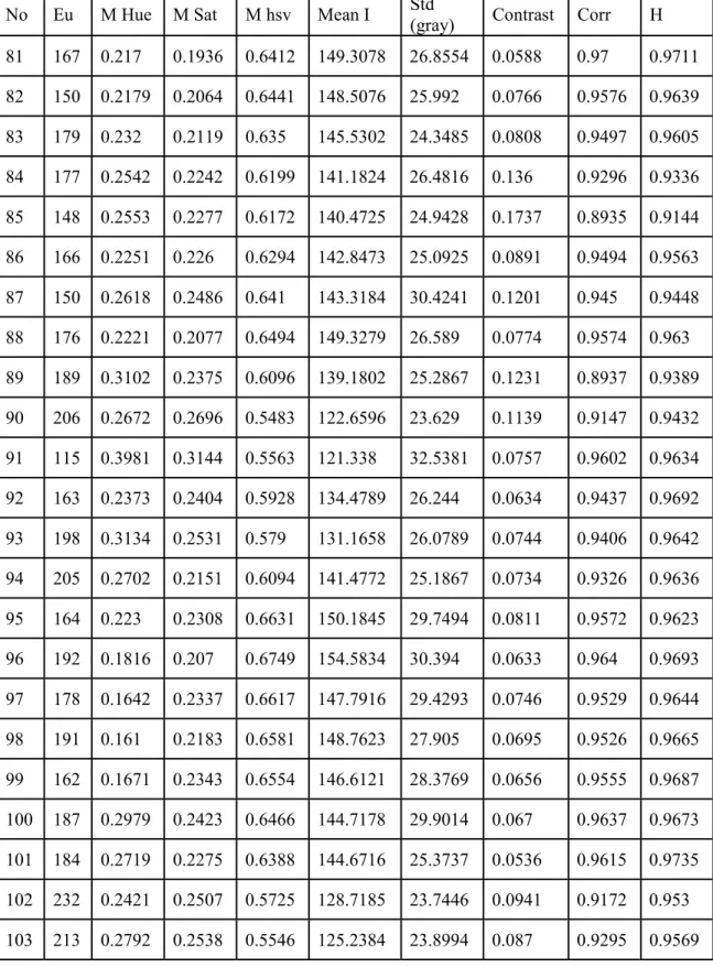
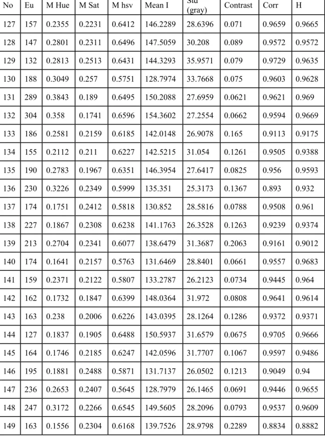
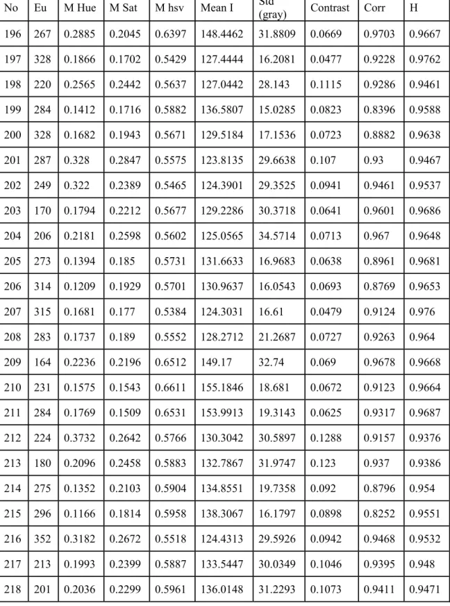
Table 1 shows the EU, Mean Hue(M Hue), Mean Sat(M Sat), Mean (hsv)(Mhsv), Mean I, Std (gray), Contrast, Correlation(Corr), Homogeneity(H).
Table 1: Image Characteristics
No Eu M Hue M Sat M hsv Mean I Std
(gray) Contrast Corr H 1 216 0.469 0.2034 0.5899 137.0815 42.2781 0.1086 0.9741 0.9482 2 166 0.5966 0.1999 0.5966 138.8615 39.9576 0.1012 0.9725 0.9513 3 174 0.6209 0.1843 0.5799 136.0405 38.2978 0.1413 0.9589 0.93 4 173 0.6391 0.1832 0.5703 133.675 37.0667 0.2628 0.905 0.8731 5 199 0.5117 0.1919 0.5593 130.0726 35.1324 0.1356 0.9357 0.9355 6 182 0.4804 0.1611 0.5715 135.8769 38.3407 0.1908 0.9252 0.9061 7 148 0.0717 0.2625 0.6274 141.2813 45.1818 0.1393 0.9652 0.9361 8 157 0.6969 0.2207 0.6208 142.5909 42.2663 0.1043 0.9716 0.952 9 263 0.7179 0.2187 0.6243 143.5927 41.1589 0.1122 0.9678 0.9447 10 219 0.6921 0.2182 0.635 145.8403 39.5054 0.1304 0.9568 0.938 11 178 0.7004 0.2075 0.6361 147.3666 41.4596 0.1185 0.964 0.9439 12 238 0.5722 0.2052 0.6365 147.7785 43.2537 0.0872 0.9767 0.9568 13 179 0.5945 0.1915 0.5954 138.8423 39.0039 0.1047 0.9698 0.9498 14 166 0.654 0.1905 0.588 137.2784 38.6073 0.1415 0.9602 0.9331 15 185 0.5097 0.165 0.5681 134.4991 36.8569 0.1435 0.9372 0.9312 16 214 0.6106 0.1795 0.594 139.7811 39.4088 0.1437 0.9614 0.9303 17 150 0.6127 0.1819 0.5836 136.8129 37.4665 0.1361 0.9599 0.9353 18 238 0.6504 0.2323 0.569 129.9555 38.7503 0.1909 0.9473 0.9063 19 190 0.6078 0.2181 0.5663 129.7329 36.056 0.1352 0.9571 0.9346 20 204 0.5301 0.1878 0.5771 134.7457 37.8622 0.1463 0.9574 0.9283 21 278 0.6218 0.294 0.5476 121.4413 43.2985 0.1795 0.9524 0.9114 22 246 0.6168 0.1971 0.5566 129.317 36.8919 0.1073 0.9505 0.9475 23 203 0.5851 0.1778 0.5489 129.0807 37.2439 0.0759 0.9654 0.9636 24 198 0.4292 0.1808 0.5579 130.3012 35.4272 0.1643 0.9329 0.9198 25 192 0.4255 0.1947 0.5511 128.21 36.0067 0.1088 0.9471 0.948 26 215 0.653 0.1934 0.5773 134.7957 38.1578 0.2439 0.9218 0.8793 27 232 0.6482 0.2285 0.5719 131.0501 37.3649 0.227 0.9309 0.8882 28 230 0.5795 0.1776 0.5704 133.9377 36.3079 0.2248 0.9228 0.8889 29 203 0.6263 0.1726 0.5782 136.4823 36.933 0.2022 0.9341 0.8993 30 241 0.635 0.2163 0.5882 135.7015 41.7475 0.1449 0.9649 0.9285 31 145 0.6174 0.1754 0.5792 136.1649 36.8535 0.1609 0.9513 0.9228 32 273 0.5576 0.2241 0.5648 129.4229 39.7874 0.1667 0.9531 0.9178 33 174 0.5613 0.1674 0.5795 136.9679 36.2017 0.2082 0.9305 0.897 34 252 0.5772 0.2306 0.5457 124.324 37.9052 0.1931 0.9327 0.9039
Table 1: Image Characteristics (continued)
No Eu M Hue M Sat M hsv Mean I Std
(gray) Contrast Corr H 35 216 0.5291 0.2511 0.5423 122.3619 39.2758 0.1896 0.9329 0.9077 36 223 0.5819 0.2471 0.5506 124.7547 40.1465 0.1905 0.9441 0.9055 37 211 0.5825 0.2201 0.5431 124.5793 37.7535 0.1721 0.9307 0.9146 38 204 0.6298 0.2002 0.5563 129.2697 37.4772 0.1572 0.9358 0.9231 39 222 0.7114 0.2129 0.5538 127.6558 36.774 0.1025 0.9543 0.95 40 211 0.527 0.1991 0.5429 125.7928 35.732 0.1245 0.9402 0.9414 41 157 0.6808 0.2043 0.5447 125.7089 35.3277 0.1266 0.9411 0.9412 42 237 0.559 0.1764 0.5493 129.2852 36.6879 0.0764 0.964 0.9626 43 128 0.4896 0.177 0.5979 140.6111 38.9198 0.1067 0.9698 0.9495 44 211 0.5112 0.2374 0.5865 134.1804 45.2475 0.1415 0.969 0.9318 45 141 0.5617 0.2053 0.5823 135.0889 40.0658 0.1176 0.9689 0.9433 46 266 0.5522 0.1968 0.5901 137.3032 38.6005 0.1166 0.9648 0.9432 47 302 0.6319 0.2717 0.5642 126.3138 40.3308 0.1115 0.9717 0.9446 48 244 0.6569 0.2316 0.5625 129.0569 35.0262 0.1348 0.9532 0.9336 49 263 0.5946 0.1911 0.5755 134.4186 38.0705 0.1855 0.9451 0.9085 50 230 0.6479 0.1764 0.5864 138.0752 37.4774 0.1686 0.9501 0.917 51 232 0.6532 0.2013 0.5751 133.6234 38.0218 0.2128 0.9359 0.8941 52 171 4067 0.2056 0.575 132.4233 35.4756 0.1508 0.9499 0.9281 53 185 0.4735 0.1945 0.6097 142.0687 38.2492 0.0921 0.9731 0.9558 54 203 0.5389 0.185 0.6139 143.247 36.806 0.0999 0.9678 0.951 55 273 0.6537 0.208 0.5947 137.1248 38.5024 0.0927 0.9731 0.9542 56 191 0.5465 0.1692 0.5369 127.4995 35.7426 0.0769 0.9642 0.9683 57 182 0.5409 0.1303 0.5693 137.5396 33.8371 0.0739 0.9564 0.9669
Table 1: Image Characteristics (continued)
No Eu M Hue M Sat M hsv Mean I Std
(gray) Contrast Corr H 58 242 0.5942 0.1677 0.5481 130.1869 36.7158 0.0793 0.9629 0.9627 59 172 0.5985 0.1656 0.5437 129.2099 35.8312 0.0588 0.9719 0.9744 60 179 0.5519 0.1754 0.5413 127.7504 35.7317 0.0942 0.9548 0.9576 61 176 0.6453 0.1765 0.5451 128.5829 35.2396 0.0872 0.959 0.96 62 209 0.4991 0.1544 0.5595 133.4499 35.1374 0.0768 0.9598 0.966 63 178 0.5276 0.169 0.563 133.503 36.5377 0.0929 0.9566 0.9577 64 248 0.6036 0.2008 0.5426 126.733 37.6485 0.0893 0.9628 0.9581 65 162 0.4894 0.1921 0.5435 127.4743 37.0528 0.0873 0.9615 0.9625 66 246 0.564 0.1896 0.5359 125.4755 36.4077 0.1639 0.9298 0.9203 67 161 0.5366 0.1988 0.5576 130.1613 36.9989 0.1495 0.9374 0.9304 68 190 0.5266 0.1905 0.5402 126.5277 36.7563 0.1173 0.9465 0.9461 69 156 0.5751 0.1612 0.538 127.9361 34.2161 0.0742 0.9648 0.9683 70 164 0.5603 0.1659 0.5668 134.3912 37.4297 0.2549 0.9041 0.8758 71 269 0.6545 0.227 0.5371 123.4888 38.5418 0.1404 0.9448 0.9319 72 171 0.5623 0.1465 0.5621 134.7047 34.5787 0.0583 0.969 0.9742 73 151 0.5676 0.2464 0.5299 121.0849 41.1425 0.0846 0.9694 0.962 74 222 0.2447 0.2252 0.6258 142.8142 24.0391 0.1028 0.9289 0.9497 75 204 0.3195 0.2745 0.6089 134.2345 30.097 0.1318 0.9445 0.9343 76 283 0.2776 0.2275 0.596 135.618 22.6763 0.0937 0.8999 0.9532 77 217 0.292 0.2453 0.5838 131.9517 26.0277 0.0556 0.956 0.9722 78 188 0.272 0.2404 0.6157 138.7309 22.9631 0.1138 0.8997 0.9434 79 196 0.2931 0.2384 0.6173 139.5133 21.5203 0.0854 0.9274 0.9573 80 191 0.2521 0.2274 0.6149 139.9566 21.4196 0.14 0.8776 0.9302
Table 1: Image Characteristics (continued)
No Eu M Hue M Sat M hsv Mean I Std
(gray) Contrast Corr H 81 167 0.217 0.1936 0.6412 149.3078 26.8554 0.0588 0.97 0.9711 82 150 0.2179 0.2064 0.6441 148.5076 25.992 0.0766 0.9576 0.9639 83 179 0.232 0.2119 0.635 145.5302 24.3485 0.0808 0.9497 0.9605 84 177 0.2542 0.2242 0.6199 141.1824 26.4816 0.136 0.9296 0.9336 85 148 0.2553 0.2277 0.6172 140.4725 24.9428 0.1737 0.8935 0.9144 86 166 0.2251 0.226 0.6294 142.8473 25.0925 0.0891 0.9494 0.9563 87 150 0.2618 0.2486 0.641 143.3184 30.4241 0.1201 0.945 0.9448 88 176 0.2221 0.2077 0.6494 149.3279 26.589 0.0774 0.9574 0.963 89 189 0.3102 0.2375 0.6096 139.1802 25.2867 0.1231 0.8937 0.9389 90 206 0.2672 0.2696 0.5483 122.6596 23.629 0.1139 0.9147 0.9432 91 115 0.3981 0.3144 0.5563 121.338 32.5381 0.0757 0.9602 0.9634 92 163 0.2373 0.2404 0.5928 134.4789 26.244 0.0634 0.9437 0.9692 93 198 0.3134 0.2531 0.579 131.1658 26.0789 0.0744 0.9406 0.9642 94 205 0.2702 0.2151 0.6094 141.4772 25.1867 0.0734 0.9326 0.9636 95 164 0.223 0.2308 0.6631 150.1845 29.7494 0.0811 0.9572 0.9623 96 192 0.1816 0.207 0.6749 154.5834 30.394 0.0633 0.964 0.9693 97 178 0.1642 0.2337 0.6617 147.7916 29.4293 0.0746 0.9529 0.9644 98 191 0.161 0.2183 0.6581 148.7623 27.905 0.0695 0.9526 0.9665 99 162 0.1671 0.2343 0.6554 146.6121 28.3769 0.0656 0.9555 0.9687 100 187 0.2979 0.2423 0.6466 144.7178 29.9014 0.067 0.9637 0.9673 101 184 0.2719 0.2275 0.6388 144.6716 25.3737 0.0536 0.9615 0.9735 102 232 0.2421 0.2507 0.5725 128.7185 23.7446 0.0941 0.9172 0.953 103 213 0.2792 0.2538 0.5546 125.2384 23.8994 0.087 0.9295 0.9569
Table 1: Image Characteristics (continued)
No Eu M Hue M Sat M hsv Mean I Std
(gray) Contrast Corr H 104 213 0.2834 0.269 0.5451 122.2185 23.2695 0.0891 0.9326 0.9558 105 210 0.2049 0.2375 0.5846 132.462 24.3383 0.0543 0.9487 0.9734 106 235 0.2949 0.2554 0.5726 129.8177 23.092 0.0891 0.9246 0.9555 107 219 0.1838 0.256 0.5551 124.0015 24.8575 0.2864 0.2052 0.6205 108 223 0.2864 0.2052 0.6205 144.0547 24.215 0.1546 0.8938 0.9231 109 138 0.293 0.2845 0.6095 133.7557 31.909 0.1052 0.9586 0.9491 110 186 0.3009 0.2253 0.6152 141.2236 28.4967 0.1411 0.9377 0.93 111 148 0.2636 0.2696 0.636 140.6216 29.3625 0.0932 0.9512 0.9585 112 246 0.2195 0.206 0.6498 149.3612 26.3923 0.0884 0.9482 0.9569 113 117 0.2712 0.2607 0.6262 139.8412 33.2303 0.088 0.9663 0.9609 114 196 0.2229 0.2471 0.5988 134.6519 29.9235 0.1337 0.9237 0.9344 115 228 0.2522 0.255 0.5976 134.3947 22.8553 0.0845 0.9213 0.958 116 184 0.2634 0.2918 0.5902 129.3042 28.9701 0.1213 0.9269 0.9423 117 231 0.2761 0.2548 0.5753 130.4267 27.9898 0.0394 0.9706 0.9806 118 129 0.2756 0.2588 0.5913 133.3336 35.1444 0.102 0.955 0.9497 119 151 0.2861 0.2571 0.6171 138.3122 29.8613 0.1354 0.939 0.9331 120 121 0.3913 0.2919 0.616 136.5191 34.7966 0.1115 0.963 0.9475 121 160 0.2771 0.2299 0.6262 142.8048 28.0875 0.0837 0.96 0.9597 122 221 0.2808 0.2486 0.5868 133.2498 25.7929 0.0699 0.9468 0.9653 123 275 0.3204 0.2299 0.6124 139.8177 25.0967 0.124 0.9233 0.938 124 209 0.2466 0.237 0.5972 136.2371 27.2486 0.0614 0.9522 0.9693 125 191 0.293 0.2443 0.6273 141.0722 29.4934 0.069 0.9695 0.9659 126 187 0.2094 0.208 0.6427 147.759 27.3671 0.0743 0.9605 0.9636
Table 1: Image Characteristics (continued)
No Eu M Hue M Sat M hsv Mean I Std
(gray) Contrast Corr H 127 157 0.2355 0.2231 0.6412 146.2289 28.6396 0.071 0.9659 0.9665 128 147 0.2801 0.2311 0.6496 147.5059 30.208 0.089 0.9572 0.9572 129 132 0.2813 0.2513 0.6431 144.3293 35.9571 0.079 0.9729 0.9635 130 188 0.3049 0.257 0.5751 128.7974 33.7668 0.075 0.9603 0.9628 131 289 0.3843 0.189 0.6495 150.2088 27.6959 0.0621 0.9621 0.969 132 304 0.358 0.1741 0.6596 154.3602 27.2554 0.0662 0.9594 0.9669 133 186 0.2581 0.2159 0.6185 142.0148 26.9078 0.165 0.9113 0.9175 134 155 0.2112 0.211 0.6227 142.5215 31.054 0.1261 0.9505 0.9388 135 190 0.2783 0.1967 0.6351 146.3954 27.6417 0.0825 0.956 0.9593 136 230 0.3226 0.2349 0.5999 135.351 25.3173 0.1367 0.893 0.932 137 174 0.1751 0.2412 0.5818 130.852 28.5816 0.0788 0.9508 0.961 138 227 0.1867 0.2308 0.6238 141.1763 26.3528 0.1263 0.9239 0.9374 139 213 0.2704 0.2341 0.6077 138.6479 31.3687 0.2063 0.9161 0.9012 140 174 0.1641 0.2157 0.5763 131.6469 28.8401 0.0661 0.9557 0.9683 141 159 0.2371 0.2122 0.5807 133.2787 26.2123 0.0734 0.9445 0.964 142 162 0.1732 0.1847 0.6399 148.0364 31.972 0.0808 0.9641 0.9614 143 163 0.238 0.2006 0.6226 143.0395 28.1264 0.1286 0.9372 0.9371 144 127 0.1837 0.1905 0.6488 150.5937 31.6579 0.0675 0.9705 0.9666 145 164 0.1746 0.2185 0.6247 142.0596 31.7707 0.1067 0.9597 0.9486 146 195 0.1881 0.2488 0.5871 131.7137 26.0502 0.1213 0.9049 0.94 147 236 0.2653 0.2407 0.5645 128.7979 26.1465 0.0691 0.9446 0.9655 148 247 0.3172 0.2266 0.6545 149.5605 28.2096 0.0793 0.9537 0.9609 149 163 0.1556 0.2304 0.6168 139.7526 28.9798 0.2289 0.8834 0.8882
Table 1: Image Characteristics (continued)
No Eu M Hue M Sat M hsv Mean I Std
(gray) Contrast Corr H 150 162 0.1824 0.2285 0.6119 138.9667 31.7688 0.2409 0.9063 0.8807 151 195 0.1972 0.2439 0.6143 138.9946 30.4384 0.2 0.9111 0.9007 152 253 0.2532 0.1726 0.5897 138.0251 29.1097 0.0771 0.9481 0.9615 153 187 0.2075 0.1737 0.5878 136.8726 32.7973 0.2134 0.9138 0.8935 154 245 0.3435 0.1721 0.591 138.3234 27.3217 0.1919 0.8842 0.9041 155 198 0.2507 0.1587 0.6359 148.928 30.5765 0.0793 0.958 0.9614 156 154 0.2119 0.1612 0.6533 153.4543 31.5612 0.0735 0.9646 0.9657 157 216 0.2639 0.1621 0.6416 150.3723 31.1337 0.0825 0.9589 0.9605 158 191 0.2175 0.1442 0.6231 147.5642 30.0635 0.0805 0.9606 0.9621 159 186 0.268 0.1467 0.6147 144.9245 29.6639 0.1027 0.9498 0.9511 160 179 0.2609 0.1509 0.655 153.8808 31.3899 0.0806 0.9586 0.9606 161 254 0.262 0.1774 0.5877 137.1565 25.8332 0.1143 0.9042 0.9432 162 250 0.3252 0.1586 0.6252 147.6128 27.493 0.0621 0.9687 0.969 163 130 0.148 0.1682 0.5941 139.1425 27.804 0.0689 0.9502 0.9678 164 220 0.2344 0.1795 0.5954 138.7813 27.6126 0.1205 0.9084 0.9403 165 155 0.2105 0.1664 0.629 147.4973 30.8364 0.0863 0.9652 0.958 166 220 0.2869 0.1831 0.6091 141.4946 28.7442 0.1454 0.9293 0.928 167 207 0.2453 0.1933 0.5751 133.4725 31.6186 0.0719 0.9617 0.9642 168 214 0.2381 0.1815 0.5771 134.3446 28.6414 0.0875 0.9435 0.9564 169 198 0.1917 0.1941 0.5759 133.5303 27.6948 0.0421 0.9735 0.9789 170 158 0.238 0.2093 0.6332 145.67 31.7132 0.0789 0.9646 0.9617 171 310 0.1769 0.1509 0.6217 146.7716 18.6396 0.1295 0.8837 0.9352 172 256 0.148 0.1535 0.6302 149.0348 17.8255 0.077 0.9219 0.9615
Table 1: Image Characteristics (continued)
No Eu M Hue M Sat M hsv Mean I Std
(gray) Contrast Corr H 173 203 0.2846 0.2414 0.5693 129.9252 29.2534 0.0867 0.9414 0.9567 174 317 0.1707 0.1849 0.5563 128.5715 16.532 0.0616 0.9012 0.9692 175 182 0.365 0.2502 0.5833 131.7569 29.9237 0.1248 0.9282 0.9386 176 331 0.4193 0.2722 0.5738 128.7323 30.4451 0.123 0.9304 0.9389 177 229 0.1483 0.1821 0.5965 137.9374 17.458 0.1099 0.8284 0.9451 178 275 0.1616 0.1943 0.5613 129.8154 17.7484 0.0593 0.91 0.9703 179 191 0.2078 0.2393 0.5745 130.1198 29.7399 0.1016 0.9417 0.9493 180 295 0.3122 0.2592 0.53 119.2902 26.0873 0.0895 0.9446 0.9557 181 230 0.119 0.1872 0.5685 131.1097 15.2141 0.0623 0.8904 0.9689 182 256 0.1992 0.1859 0.5852 136.9356 21.5204 0.0523 0.9352 0.9739 183 194 0.2179 0.2033 0.5798 133.8749 31.1211 0.0651 0.9612 0.9683 184 192 0.2139 0.1937 0.5757 133.0793 27.438 0.0648 0.9514 0.9684 185 215 0.2675 0.2058 0.637 147.8061 31.9809 0.0566 0.9761 0.9717 186 361 0.1234 0.1225 0.6445 154.1711 11.8131 0.0513 0.9154 0.9743 187 186 0.2353 0.2231 0.6362 146.018 32.3992 0.0726 0.97 0.9638 188 250 0.1428 0.1649 0.6468 152.3624 15.4336 0.0499 0.9345 0.9751 189 188 0.2196 0.2104 0.6391 147.3809 31.7548 0.073 0.967 0.9638 190 259 0.137 0.1605 0.6439 151.42 15.2013 0.0583 0.9139 0.9708 191 195 0.2553 0.2142 0.6368 145.9457 30.8301 0.0711 0.9652 0.9645 192 254 0.3325 0.2142 0.6433 148.4518 31.3069 0.091 0.9601 0.9555 193 226 0.1659 0.1612 0.6174 145.1883 20.1209 0.2197 0.7952 0.8902 194 222 0.219 0.232 0.5937 135.8742 30.0892 0.0608 0.9618 0.9698 195 203 0.3318 0.2587 0.5373 121.5691 27.4338 0.0783 0.9568 0.9611
Table 1: Image Characteristics (continued)
No Eu M Hue M Sat M hsv Mean I Std
(gray) Contrast Corr H 196 267 0.2885 0.2045 0.6397 148.4462 31.8809 0.0669 0.9703 0.9667 197 328 0.1866 0.1702 0.5429 127.4444 16.2081 0.0477 0.9228 0.9762 198 220 0.2565 0.2442 0.5637 127.0442 28.143 0.1115 0.9286 0.9461 199 284 0.1412 0.1716 0.5882 136.5807 15.0285 0.0823 0.8396 0.9588 200 328 0.1682 0.1943 0.5671 129.5184 17.1536 0.0723 0.8882 0.9638 201 287 0.328 0.2847 0.5575 123.8135 29.6638 0.107 0.93 0.9467 202 249 0.322 0.2389 0.5465 124.3901 29.3525 0.0941 0.9461 0.9537 203 170 0.1794 0.2212 0.5677 129.2286 30.3718 0.0641 0.9601 0.9686 204 206 0.2181 0.2598 0.5602 125.0565 34.5714 0.0713 0.967 0.9648 205 273 0.1394 0.185 0.5731 131.6633 16.9683 0.0638 0.8961 0.9681 206 314 0.1209 0.1929 0.5701 130.9637 16.0543 0.0693 0.8769 0.9653 207 315 0.1681 0.177 0.5384 124.3031 16.61 0.0479 0.9124 0.976 208 283 0.1737 0.189 0.5552 128.2712 21.2687 0.0727 0.9263 0.964 209 164 0.2236 0.2196 0.6512 149.17 32.74 0.069 0.9678 0.9668 210 231 0.1575 0.1543 0.6611 155.1846 18.681 0.0672 0.9123 0.9664 211 284 0.1769 0.1509 0.6531 153.9913 19.3143 0.0625 0.9317 0.9687 212 224 0.3732 0.2642 0.5766 130.3042 30.5897 0.1288 0.9157 0.9376 213 180 0.2096 0.2458 0.5883 132.7867 31.9747 0.123 0.937 0.9386 214 275 0.1352 0.2103 0.5904 134.8551 19.7358 0.092 0.8796 0.954 215 296 0.1166 0.1814 0.5958 138.3067 16.1797 0.0898 0.8252 0.9551 216 352 0.3182 0.2672 0.5518 124.4313 29.5926 0.0942 0.9468 0.9532 217 213 0.1993 0.2399 0.5887 133.5447 30.0349 0.1046 0.9395 0.948 218 201 0.2036 0.2299 0.5961 136.0148 31.2293 0.1073 0.9411 0.9471
Table 1: Image Characteristics (continued)
No Eu M Hue M Sat M hsv Mean I Std
(gray) Contrast Corr H 219 183 0.2533 0.2313 0.5826 133.1629 30.998 0.1003 0.9415 0.95 220 307 0.147 0.1742 0.5771 133.8593 16.4108 0.063 0.89 0.9685 221 267 0.163 0.1783 0.5391 126.5978 15.351 0.0479 0.9314 0.9761 222 250 0.371 0.2711 0.5479 122.2471 27.7139 0.1034 0.9374 0.9484 223 245 0.346 0.2511 0.5675 128.5259 29.2258 0.0953 0.9449 0.9531 224 246 0.173 0.1923 0.5872 135.9832 17.508 0.0717 0.876 0.9641 225 236 0.2374 0.2505 0.5758 130.4548 29.3092 0.0985 0.9413 0.9508 226 268 0.1589 0.2176 0.5592 127.0419 16.7429 0.0729 0.889 0.9638 227 223 0.1203 0.1843 0.5712 132.3307 15.432 0.0544 0.9059 0.9728 228 125 0.4296 0.3406 0.3724 80.6708 35.08 0.0588 0.9793 0.9706 229 276 0.4704 0.3594 0.3445 73.0371 33.3848 0.069 0.9767 0.9655 230 184 0.4608 0.3644 0.342 73.0784 32.6151 0.0703 0.9733 0.9648 231 222 0.1915 0.2263 0.4511 102.4717 24.734 0.068 0.9296 0.9661 232 179 0.1937 0.2394 0.4485 101.3462 23.9068 0.0706 0.9252 0.9649 233 187 0.3521 0.2511 0.4193 94.8307 23.8656 0.0855 0.9272 0.9572 234 382 0.278 0.2422 0.4308 97.7119 22.582 0.0563 0.9453 0.9719 235 207 0.1985 0.2412 0.4421 99.505 23.5396 0.0721 0.9309 0.9639 236 274 0.2585 0.25 0.4253 95.8784 21.6108 0.066 0.935 0.967 237 210 0.2623 0.221 0.4835 110.351 25.2659 0.2011 0.8857 0.9 238 148 0.359 0.2043 0.4582 105.8264 24.9651 0.0876 0.9099 0.9565 239 270 0.2708 0.1965 0.4776 110.877 24.4717 0.1395 0.8771 0.9302 240 231 0.3281 0.1969 0.461 106.7023 22.5692 0.0743 0.9053 0.9629 241 241 0.2452 0.2309 0.4472 102.6709 22.4223 0.0565 0.9421 0.9718
Table 1: Image Characteristics (continued)
No Eu M Hue M Sat M hsv Mean I Std
(gray) Contrast Corr H 242 214 0.185 0.2368 0.4765 107.3609 24.0996 0.1281 0.8652 0.936 243 318 0.3332 0.2639 0.471 104.7044 23.4035 0.1253 0.8785 0.9374 244 248 0.2762 0.232 0.4593 103.9963 21.8725 0.0921 0.8895 0.954 245 140 0.212 0.242 0.4569 102.8657 24.7478 0.0879 0.907 0.9566 246 300 0.4162 0.2887 0.4406 96.7534 22.313 0.1158 0.8831 0.9421 247 248 0.2528 0.2199 0.4487 102.6697 23.7028 0.0783 0.92 0.9609 248 215 0.2753 0.2599 0.4393 97.7628 20.4903 0.0903 0.8973 0.9549 249 234 0.1925 0.2757 0.4393 97.6049 22.0031 0.0926 0.8968 0.9537 250 260 0.4122 0.2618 0.4129 92.8019 19.5636 0.0966 0.9012 0.9517 251 179 0.2428 0.2384 0.4004 90.8963 21.1342 0.0909 0.9142 0.9546 252 179 0.2805 0.226 0.4695 106.5261 22.0415 0.1147 0.8726 0.943 253 209 0.1926 0.2539 0.4666 102.9234 24.2986 0.1678 0.8566 0.9163 254 296 0.3889 0.2569 0.4641 104.2286 19.8208 0.1216 0.8254 0.9392 255 282 0.2926 0.261 0.4649 103.957 21.0551 0.1184 0.8683 0.9408 256 246 0.3712 0.2711 0.5478 122.2195 27.6923 0.1037 0.9371 0.9483 257 245 0.346 0.2511 0.5675 128.5259 29.2258 0.0953 0.9449 0.9531 258 240 0.1755 0.192 0.5871 135.9844 17.7009 0.0703 0.8794 0.9649 259 232 0.238 0.2506 0.5755 130.3813 29.2884 0.098 0.9415 0.951 260 221 0.1199 0.1845 0.5708 132.1815 15.4369 0.0552 0.9047 0.9724
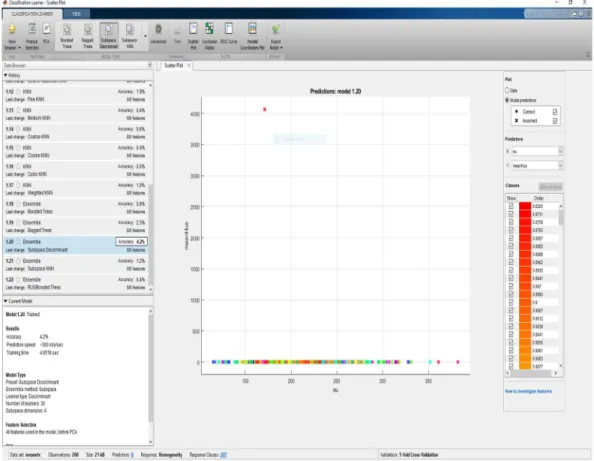
The Ensemble Subspace Discriminant shows that the accuracy is 4.2%, the prediction speed 300 observations/seconds and the training time as 4.9518 seconds. This was the best result for the classification using Image Characteristics as a variable. Figure 1 shows the result of the ensemble subspace discriminant classifier.
Figure 1: Mean Ensemble Subspace Discriminant
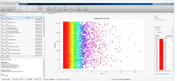
Then, the stats variable was classified for various models. Figure 2 shows the scatter plot for the stats variable without classification.
Figure 2: Scatter Plot Stats
The result of the classification model of the Fine tree classifier was 69.0% accuracy, the prediction speed 6100 observations/sec and the training time as 82.901sec. This was the best result for the classification using stats as a variable. Figure 3 shows the result of the Fine tree classifier.
Figure 3: Scatter Plot Stats Fine Tree Model
Since the results of stats and image characteristics were not as expected it was decided to investigate the k-means segmentation as given in the following sections.
4.2. Evaluation Measures
The L_blue variable having 2591/2591 features from the segmentation is used for the classification task. The experiments are run using 20 models and the accuracy in %, prediction speed in observations/sec, and the training time in sec was used as evaluation measures.
4.3. Results
At first, the identification and segmentation of WBCs were done by means of image clustering. Color features are extracted from the nucleus in the whole images, each of which contains multiple nuclei [36]. The dataset ALL IDB1 was used. The images generated by digital microscopes are usually in RGB color space, which is difficult to segment. In practice, various reasons such as camera settings, varying illumination, and aging stain may cause the blood cells and image background to vary greatly with respect to color and intensity. For making the cell segmentation robust with respect to these variations, reducing the memory requirement and improving the computational time, an adaptive procedure is used:
Figure 4 shows the original image (RGB), and Figure 5 shows the gray image.
Figure 5: Gray Image
The RGB input image is converted into the CIELAB format or more correctly, the CIEL*a*b* color space. This color space consists of a luminosity layer L*, which represents the lightness of the color, chromaticity layers, a* represents its position between red/magenta and green, and b* represents its position between yellow and blue. Since all the color information is in the a* and b* layers, we use these two components for nucleus segmentation. Moreover, the perceptual difference between the colors is proportional to the Cartesian distance in the CIELAB color space. Therefore, the color differences between two samples can be calculated using the Euclidean distance. L*a*b produces a proportional change visually for a change of the same amount in color value due to its perceptual uniformity. Therefore, every minute difference in the color value is noticed visually. The image is converted to the L*a*b* color space using rgb2lab and classify the colors in the 'a*b*' space using K-Means Clustering. Clustering is a way to separate groups of objects. K-means clustering treats each object as having a location in space. It finds partitions such that objects within each cluster are as close to each other as possible, and as far as possible from the objects in other clusters. K-means clustering requires to specify the
number of clusters to be partitioned and a distance metric to quantify how close two objects are to each other.
Since the color information exists in the 'a*b*' color space, our objects are pixels with 'a*' and 'b*' values. The data is converted into data type single for use with imsegkmeans to cluster the objects into three clusters. The clustering is repeated 3 times to avoid local minima.
For every object as input, imsegkmeans returns an index, or a label, corresponding to a cluster. Label every pixel in the image with its pixel label. Images are created that segment the image by color. Using pixel labels, the objects are separated in I by color, which will result in three images - Cluster1, Cluster2, Cluster3. Figure 6 shows Cluster1, Figure 7 shows Cluster 2, and Figure 8 shows Cluster 3, respectively.
Figure 7: Cluster 2
To segment the nuclei, Cluster 3 contains the blue objects. There are dark and light blue objects. Dark blue is separated from light blue using the 'L*' layer in the L*a*b* color space. The cell nuclei are dark blue.
The 'L*' layer contains the brightness values of each color. The brightness values of the pixels in this cluster are extracted and thresholded with a global threshold using im binarize. The mask is light blue and gives the indices of light blue pixels.
The mask of blue objects, mask3 are copied, then the light blue pixels from the mask are removed. Afterward, the new mask is applied to the original image and the result is displayed. Only dark blue cell nuclei are visible.
During the segmentation, all the images of the training datasets were saved as respective figure a, b, c, d, e, f. Figure 9 shows the Blue nuclei. In this system, the color-based clustering segmentation is performed for extracting the nuclei of the leukocytes.
4.3.1. Results of Segmentation
Figure 9: Blue Nuclei
The segmented output of the image obtained after applying the K-means clustering algorithm is shown in Figure 9.
4.4. Characteristics of Classifier Types
For choosing the best classifier type for the problem. Table 2 is showing the typical characteristics of different supervised learning algorithms. The table was used as a guide for our final choice of algorithms. The decision is a tradeoff between speed, memory usage, flexibility, and interpretability. The best classifier type depends on our data [39].
Table 2: Characteristics of Classifier Types Classifier Prediction
Speed Memory Usage Interpretability All predictors numeric All predictors categorical Some categorical, some numeric Decision
Trees Fast 0.01second Small 1MB Easy Yes Yes Yes Discriminant
Analysis Fast 0.01second Small for linear, large for quadratic
Easy Yes No No Logistic
Regression Fast 0.01 second Medium 4MB Easy Yes Yes Yes Support
Vector Machines
Medium 1 second for linear. Slow for others Medium for linear. All others: a medium for multiclass, Large 100MB for binary. Easy for Linear SVM. Hard for all other kernel types.
Yes Yes Yes
Nearest
Neighbor Slow 100 seconds for cubic. Medium for others
Medium 4MB Hard Euclidean distance only Hamming distance only No
Ensembles Fast to medium depending on the choice of algorithm Low to high depending on the choice of algorithm
Hard Yes Yes, except Subspace Discriminant
Yes, except any Subspace Naive Bayes Medium for
simple distributions. Slow for kernel distributions or high-dimensional data Small for simple distributions. Medium for kernel distributions or high-dimensional data
4.4.1. Decision Trees
Decision trees are easy to interpret, fast for fitting and prediction, and low on memory usage, but they can have low predictive accuracy. The idea is to grow simpler trees to prevent overfitting. Control the depth with the Maximum number of splits set [38]. Table 3 shows different types of decision trees classifiers.
Table 3: Different Types of Decision Trees Classifiers Classifier
Type
Prediction Speed
Memory
Usage Interpretability Model Flexibility Coarse
Tree
Fast Small Easy Low
Few leaves to make coarse distinctions between classes (maximum number of splits is 4).
Medium
Tree Fast Small Easy Medium Medium number of leaves for finer distinctions between classes (maximum number of splits is 20).
Fine
Tree Fast Small Easy High Many leaves to make many fine
distinctions between classes (maximum number of splits is 100).
4.4.2. Support Vector Machines
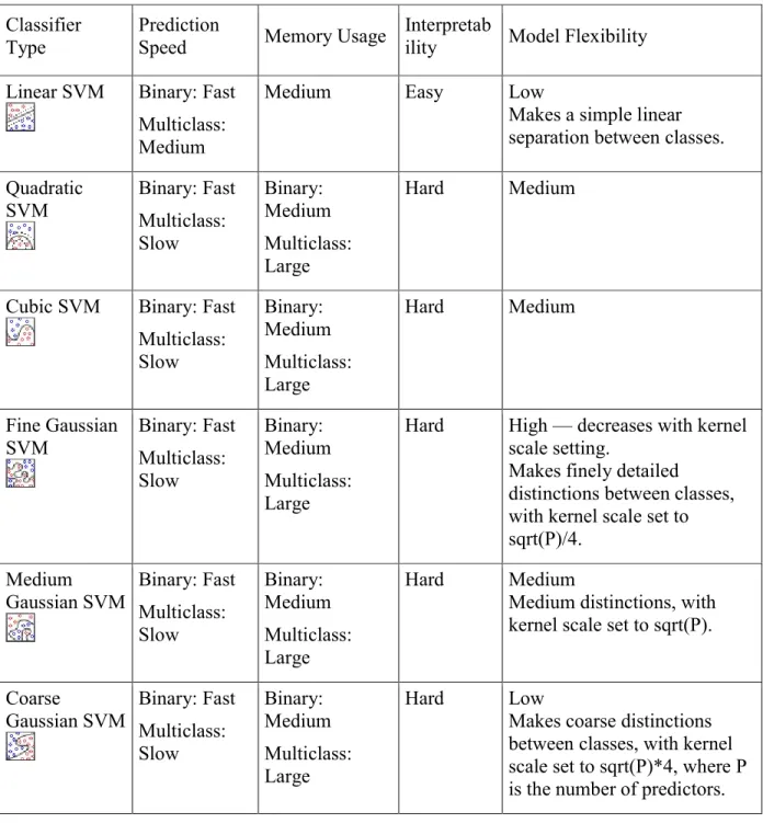
In Classification Learner, you can train SVMs when your data has two or more classes. Table 4 shows the different types of Support Vector Machines Classifiers.
Table 4: Different Types of Support Vector Machines Classifiers Classifier
Type
Prediction
Speed Memory Usage
Interpretab
ility Model Flexibility Linear SVM Binary: Fast
Multiclass: Medium
Medium Easy Low
Makes a simple linear separation between classes. Quadratic SVM Binary: Fast Multiclass: Slow Binary: Medium Multiclass: Large Hard Medium
Cubic SVM Binary: Fast Multiclass: Slow Binary: Medium Multiclass: Large Hard Medium Fine Gaussian
SVM Binary: Fast Multiclass: Slow
Binary: Medium Multiclass: Large
Hard High — decreases with kernel scale setting.
Makes finely detailed
distinctions between classes, with kernel scale set to sqrt(P)/4. Medium Gaussian SVM Binary: Fast Multiclass: Slow Binary: Medium Multiclass: Large Hard Medium
Medium distinctions, with kernel scale set to sqrt(P).
Coarse
Gaussian SVM Binary: Fast Multiclass: Slow Binary: Medium Multiclass: Large Hard Low
Makes coarse distinctions between classes, with kernel scale set to sqrt(P)*4, where P is the number of predictors.
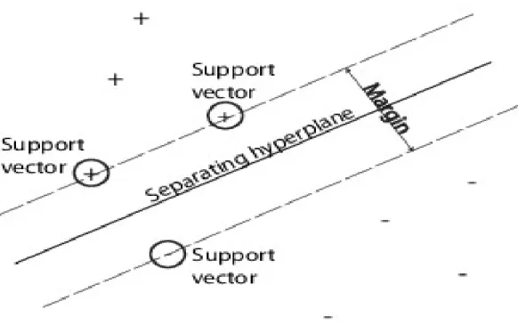
An SVM classifies data by finding the best hyperplane that separates data points of one class from those of the other class. The best hyperplane for an SVM means the one with the largest margin between the two classes. Margin means the maximal width of the slab parallel to the hyperplane that has no interior data points.
The support vectors are the data points that are closest to the separating hyperplane; these points are on the boundary of the slab. The following figure illustrates these definitions, with + indicating data points of type 1, and – indicating data points of type –1.
Figure 10 shows Support Vectors
Figure 10: Support Vectors
SVMs can also use a soft margin, meaning a hyperplane that separates many, but not all data points.
4.4.3. Nearest Neighbor Classifiers
Nearest neighbor classifiers typically have good predictive accuracy in low dimensions, but might not in high dimensions. They have high memory usage and are not easy to interpret. Table 5 shows different types of nearest neighbor classifiers.
Table 5: Different Types of Nearest Neighbor Classifiers
Classifier Type Prediction Speed Memory Usage Interpretability Model Flexibility
Fine KNN Medium Medium Hard Finely detailed distinctions between classes. The number of neighbors is set to 1. Medium KNN Mediu Medium Hard Medium distinctions between classes. The
number of neighbors is set to 10. Coarse KNN Medium Medium Hard Coarse distinctions between classes. The
number of neighbors is set to 100.
Cosine KNN Medium Medium Hard Medium distinctions between classes, using a Cosine distance metric. The number of neighbors is set to 10.
Cubic KNN Slow Medium Hard Medium distinctions between classes, using a cubic distance metric. The number of neighbors is set to 10.
Weighted KNN Medium Medium Hard Medium distinctions between classes, using a distance weight. The number of neighbors is set to 10.
k-Nearest Neighbor classification is categorizing query points based on their distance to points (or neighbors) in a training dataset can be a simple yet effective way of classifying new points. You can use various metrics to determine the distance. Given a set X of n points and a distance function, k-nearest neighbor (kNN) search lets you find the k closest points in X to a query point or set of points. kNN-based algorithms are widely used as benchmark machine learning rules.
4.4.4. Ensemble Classifiers
Ensemble classifiers meld results from many weak learners into one high-quality ensemble model. Qualities depend on the choice of algorithm. Table 6 shows different types of Ensemble Classifiers
Table 6: Different Types of Ensemble Classifiers
Classifier Type Predictio n Speed Memo ry Usage Interpret
ability Ensemble Method Model Flexibility Boosted
Trees
Fast Low Hard AdaBoost,
with Decision Tree learners
Medium to high — increases with Number of learners o a Maximum number of a split set.
Bagged Trees
Medium High Hard Random forest Bag, with Decision Tree learners High — increases with Number of learners setting. Subspace Discrimina nt
Medium Low Hard Subspace,
with Discriminant learners
Medium — increases with Number of learners setting.
Good for many predictors Subspace
KNN Medium Medium Hard Subspace, with Nearest Neighbor learners
Medium — increases with Number of learners setting.
Good for many predictors RUS Boost
Trees
Fast Low Hard RUS Boost,
with Decision Tree learners
Medium — increases
with Number of learners or a Maximum number of a split set.
Good for skewed data (with many more observations of 1 class)
4.5. Results of Classification
Following the classification, cross-validation is used for evaluating and comparing the different learning algorithms. Cross-validation is a technique for judging how the results of the statistical analysis will generalize to an independent data set.
Experiments were ran using 20 models namely Fine Tree, Medium Tree, Coarse Tree, Linear SVM, Quadratic SVM, Cubic SVM, Fine Gaussian SVM, Medium Gaussian SVM, Coarse Gaussian SVM, Fine KNN, Medium KNN, Coarse KNN, Cosine KNN, Cubic KNN, Weighted KNN, Ensemble Boosted Trees, Ensemble Bagged Trees, Ensemble Subspace Discriminant, Ensemble Subspace KNN, Ensemble RUS Boosted Trees as also given in the list below.
List of Models Used for Classification Model 1. Fine Tree 2. Coarse Tree 3. Quadratic Discriminant 4. Fine Gaussian SVM 5. Coarse Gaussian SVM 6. Medium KNN 7. Cosine KNN 8. Weighted KNN
9. Ensemble Bagged Trees 10. Ensemble Subspace KNN 11. Medium Tree
12. Linear Discriminant 13. Cubic SVM 14. Medium Gaussian SVM 15. Fine KNN 16. Coarse KNN 17. Cubic KNN
18. Ensemble Boosted Trees
19. Ensemble Subspace Discriminant 20. Ensemble RUS Boosted Trees
First, the experiment was run using 20 models with the data set stats with observations 17,717, Predictors 18, Response Perimeter, Response Classes 2,372, and the result of the training for the Fine Tree classifier accuracy was 69% with prediction speed ~6,100 observations /sec and training time was 82.901 sec.
The result of the classification model of the Fine Tree classifier with the L_Blue dataset was 99.7% accuracy, the prediction speed 1,100 observations/sec and the training time as 8.6611 sec. This was the best result for the classification using stats as the variable.
Figure 11: Fine Tree
Then, the experiment was run using 20 models with data sets L_Blue. Of the 20 models, only 10 models had an accuracy of 99.9%. These 10 models namely Linear SVM, Medium Gaussian SVM, Coarse Gaussian SVM, Medium KNN, Coarse KNN, Cosine KNN, Cubic KNN, Weighted KNN, Ensemble Boosted Trees, Ensemble Bagged Trees. Among these the prediction speed and training time is different and these models are evaluated based on the prediction speed and training time. Table 7 shows the results of the different classifier models showing accuracy, prediction speed, and training time.
Model Accuracy (%) Prediction speed (observations/sec) Training time (sec) Fine Tree 99.7 ~1200 6.1802 Medium Tree 99.7 ~1200 5.8724 Coarse Tree 99.7 ~1200 5.8936 Linear SVM 99.9 ~1100 20.499 Quadratic SVM 99.7 ~710 24.218 Cubic SVM 99.3 ~710 24.094 Fine Gaussian SVM 95.1 ~540 36.778 Medium Gaussian SVM 99.9 ~760 24.621 Coarse Gaussian SVM 99.9 ~750 24.188 Fine KNN 99.7 ~490 15.87 Medium KNN 99.9 ~500 15.159 Coarse KNN 99.9 ~500 15.327 Cosine KNN 99.9 ~470 15.299 Cubic KNN 99.9 ~86 78.014 Weighted KNN 99.9 ~520 14.889
Ensemble Boosted Trees 99.9 ~1200 6.8817
Ensemble Bagged Trees 99.9 ~720 18.466
Ensemble Subspace
Discriminant 99.8 ~160 227.47
Ensemble Subspace KNN 99.8 ~47 136.58
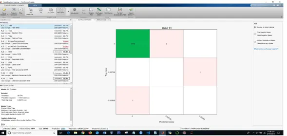
The result of the classification model of the Coarse KNN classifier with the L_Blue dataset was 99.0% accuracy, the prediction speed 480 observations/sec and the training time as 15.395 sec. Figure 12 shows the result of the Coarse KNN classifier with the confusion matrix, and Figure 13 shows the result of the Coarse KNN classifier showing the ROC curve.
Figure 12: Coarse KNN
The result of the classification model of the Cosine KNN classifier with the L_Blue dataset was 99.9% accuracy, the prediction speed 470 observation /sec and the training time as 15.299 sec. Figure 14 shows the result of the Cosine KNN classifier with the confusion matrix, and Figure 15 shows the result of the Cosine KNN classifier and the resulting ROC curve.
Figure 14: Cosine KNN
The result of the classification model of the Cubic KNN classifier with the L_Blue dataset was 99.9% accuracy, the prediction speed 86 observations/sec and the training time as 78.014 sec. Figure 16 shows the result of the Cubic KNN classifier with the resulting confusion matrix, and Figure 17 shows the result of the Cubic KNN classifier and the ROC curve.
Figure 16: Cubic KNN
The result of the classification model of the Ensemble Bagged Trees Confusion Matrix classifier with the L_Blue dataset was 99.9 % accuracy, the prediction speed 720
observations/sec and the training time as 18.466 sec. Figure 18 shows the result of the Ensemble Bagged Trees Confusion Matrix classifier with a confusion matrix, and Figure 19 shows the result of the Ensemble Bagged Trees Confusion Matrix classifier with a ROC curve.
Figure 18: Ensemble Bagged Trees Confusion Matrix
The result of the classification model of the Ensemble Boosted Trees classifier with the L_Blue dataset was 99.9 % accuracy, the prediction speed 1,200 observations/sec and the training time as 6.8817 sec. Figure 20 shows the result of the Ensemble Boosted Trees classifier with the confusion matrix.
Figure 20: Ensemble Boosted Trees
The result of the classification model of the KNN Medium classifier with the L_Blue dataset was 99.9% accuracy, the prediction speed 500 observations/sec and the training time as 15.150 sec. Figure 21 shows the result of the KNN Medium classifier with a confusion matrix, and Figure 22 shows the result of the KNN Medium classifier with the ROC curve.
Figure 22: KNN Medium ROC
The result of the classification model of the Linear SVM classifier with the L_Blue dataset was 99.9% accuracy, the prediction speed 1100 observations/sec and the training time as 20.499 sec. Figure 23 shows the result of the Linear SVM classifier with a confusion matrix, and Figure 24 shows the result of the Linear SVM classifier with the ROC curve.
Figure 24: Linear SVM ROC
The result of the classification model of the SVM Medium Gaussian classifier with the L_Blue dataset was 99.9 % accuracy, the prediction speed 760 observations/sec and the training time as 24.621 sec. Figure 25 shows the result of the SVM Medium Gaussian classifier with a confusion matrix, and Figure 26 shows the result of the SVM Medium Gaussian classifier with a ROC curve.
Figure 26: SVM Medium Gaussian ROC
The result of the classification model of the SVM Coarse Gaussian classifier with the L_Blue dataset was 99.9% accuracy, the prediction speed 750 observations/sec and the training time as 24.188 sec. Figure 27 shows the result of the SVM Coarse Gaussian classifier.
The result of the classification model of the Weighted KNN classifier with the L_Blue dataset was 99.9 % accuracy, the prediction speed 520 observations/sec, and the training time as 14.889 sec. Figure 28 shows the result of the Weighted KNN classifier with a confusion matrix, and Figure 29 shows the result of the Weighted KNN classifier with the ROC curve.
Figure 28: Weighted KNN
Figure 30 shows the bar chart for the training time. From the bar chart, the maximum training time is used by Ensemble Subspace Discriminant and the least is used by the Fine Tree, Medium Tree, Coarse Tree models.
Figure 30: Bar Chart Model - Training Time
Figure 31 shows the bar chart of the accuracy showing an accuracy of 99.9% for most of the models. Fine Gaussian SVM and Ensemble RUS Boosted Trees have lesser accuracy values compared to other models.
Figure 32 shows the stacked plot of accuracy vs training time. In the plot, the accuracy decreases and the training time increases for some models but it is not a general pattern. Fine Gaussian SVM (7) has an increased training time and the least accuracy. Cubic KNN (14) and Ensemble Subspace Discriminant (18) had an increased training time but the accuracy was not affected.
Figure 32: Stacked Plot Accuracy vs Training Time
Figure 33 shows the stacked plot of model and training time.
Figure 34 shows the stacked plot of model and accuracy.
Figure 34: Stacked Plot Model and Accuracy
Figure 35 shows the area plot of accuracy and training time.
Figure 35: Area Plot Accuracy and Training Time
Figure 36 shows the X bar control chart of accuracy and prediction speed. There is a drastic decrease in the accuracy at two points, but the pattern is not followed by all models.
Figure 36: The X Bar Control Chart Accuracy and Prediction Speed
Figure 37 shows the scatter plot of accuracy and training time. Most models achieved an accuracy of around 99.5% to 100%, and the training time is less than 50 sec. In a few models, the accuracy is decreased but the training time is less than 50 sec. But in some other models, the accuracy is above 99.5% but the training time needed is longer than 50 secs.
Figure 38 shows the histogram of the test data.
Figure 38: Histogram Test Data
Figure 39 shows the histogram of the train data.
Figure 40 shows the histogram of the L_blue.
Figure 40: Histogram L_blue
Figure 41 shows the contour pixel_label.
Of all the models, the Ensemble Boosted Trees model has the least training time and the best prediction speed. If the prediction speed is taken into consideration then Linear SVM comes second and if training time is given priority then KNN (Medium, Coarse, Cosine and Weighted) are the second. If the worst performance based on the training time and prediction speed is taken into consideration then Cubic KNN, Coarse Gaussian SVM, and Medium Gaussian SVM are last, second last and third last, respectively.
Since there were 10 models with 99.9 % accuracy without PCA, it was difficult to find a model which would be best to choose from. The dataset L_blue was again classified using Principal Component Analysis (PCA) as the preprocessing method for all the 20 models. PCA reduces the dimensionality of data by replacing several correlated variables with a new set of variables that are linear combinations of the original variables. With 95% variance, there were 11 models with 99.9% accuracy, so the variance was increased to 99.9%.
The models were run on 271 features and 1943 observations using 99.9% variance, there were seven models namely Medium KNN, Coarse KNN, Cosine KNN, Cubic KNN, Weighted KNN, Ensemble Boosted trees and Ensemble Bagged trees which had 99.9% accuracy.
Cubic KNN has the maximum training time and the least prediction speed while all the others had approximately the same prediction speed and training time. The Confusion Matrix and Receiver operating characteristic (ROC) curve were taken into consideration to select the best model.
Table 8 shows the results of the different classifier models showing accuracy, prediction speed, and training time using PCA with 99.9 variances.
Table 8: Model, Accuracy and Training Time using PCA Model Accuracy (%) Prediction speed
(observations/sec) Training time(sec) Medium KNN 99.9 ~1600 19.083 Coarse KNN 99.9 ~1500 19.89 Cosine KNN 99.9 ~1600 19.738 Cubic KNN 99.9 ~220 41.914 Weighted KNN 99.9 ~1600 19.37 Ensemble Boosted Trees 99.9 ~1900 18.89 Ensemble Bagged Trees 99.9 ~1700 21.436
4.6. Result of Classification using PCA
The result of the classification model of the KNN Medium classifier using PCA with the L_Blue dataset was 99.9% accuracy, the prediction speed was 1600 observations/sec, and the training time was 19.083 sec. Figure 42 shows the result of the KNN Medium classifier using PCA with ROC, and Figure 43 shows the result of the KNN Medium classifier using PCA with the confusion matrix.
Figure 43: Medium KNN using PCA with Confusion Matrix
The result of the classification model of the Weighted KNN classifier using PCA with the L_Blue dataset was 99.9% accuracy, the prediction speed was 1600 observations/sec, and the training time was 19.37 sec. Figure 44 shows the result of the Weighted KNN classifier using PCA with a ROC curve. Figure 45 shows the result of the Weighted KNN classifier using PCA with the confusion matrix.
Figure 45: Weighted KNN using PCA with Confusion Matrix
The result of the classification model of the Ensembled Bagged classifier using PCA with the L_Blue dataset was 99.9% accuracy, the prediction speed 1700 observations/sec, and the training time was 121.436 sec. Figure 46 shows the result of the Ensembled Bagged classifier using PCA with a ROC curve. Figure 47 shows the result of the Ensembled Bagged classifier using PCA with the confusion matrix.
Figure 47: Ensembled Bagged using PCA with Confusion Matrix
Of all the remaining models Weighted KNN was the only model with 100% Positive Predictive value in the Confusion matrix and the ROC curve was showing maximum true positive value with zero positive rates. All other models were also good as they were showing more than 99% Positive Predictive value and less than 1% False discovery rate. So weighted KNN was chosen as the best model. The test data was segmented through k-means clustering and the L_blue3 dataset was used to test the data. The L_blue3 has the last column as a response which was not used to test the data. As the data used should have the same number of columns as the train data. Y fit is the expected result, which is equal to the response column of the L_blue3 of the test data. Hence the result was 100 %. But if we use the new dataset then the result can be different.