Confidence bands in quantile regression and generalized dynamic semiparametric factor models

(1)

Confidence Bands in Quantile Regression and

Generalized Dynamic Semiparametric Factor Models

D I S S E R T A T I O N

zur Erlangung des akademischen Grades

Doctorate

im Fach Statistics and Econometrics

eingereicht an der

Wirtschaftswissenschaftlichen Fakultät

Humboldt-Universität zu Berlin

von

Msc. Song Song

18.07.1984

Präsident der Humboldt-Universität zu Berlin:

Prof. Dr. Dr. h.c. Christoph Markschies

Dekan der Wirtschaftswissenschaftlichen Fakultät:

Prof. Oliver Günther, Ph.D.

Gutachter:

1. Prof. Dr. Wolfgang Karl Härdle

2. Prof. Dr. Ya’acov Ritov

eingereicht am:

07.06.2010

(2)

(3)

The topic this thesis deals with is complex, but very interesting. I want to thank my supervisor Prof. Dr. Wolfgang Karl Härdle and Prof. Dr. Ya’acov Ritov for the great opportunities to learn from them and the support during the production of this thesis. To overcome all of the theoretical and empirical challenges, I also want to thank Dr. T. Vogel, Peter Bickel for their great presence.

(4)

(5)

Abstract

In many applications it is necessary to know the stochastic fluctuation of the max-imal deviations of the nonparametric quantile estimates, e.g. for various parametric models check. Uniform confidence bands are therefore constructed for nonpara-metric quantile estimates of regression functions. The first method is based on the strong approximations of the empirical process and extreme value theory. The strong uniform consistency rate is also established under general conditions. The second method is based on the bootstrap resampling method. It is proved that the bootstrap approximation provides a substantial improvement. The case of multidi-mensional and discrete regressor variables is dealt with using a partial linear model. A labor market analysis is provided to illustrate the method.

High dimensional time series which reveal nonstationary and possibly periodic be-havior occur frequently in many fields of science, e.g. macroeconomics, meteorology, medicine and financial engineering. One of the common approach is to separate the modeling of high dimensional time series to time propagation of low dimensional time series and high dimensional time invariant functions via dynamic factor analy-sis. We propose a two-step estimation procedure. At the first step, we detrend the time series by incorporating time basis selected by the group Lasso-type technique and choose the space basis based on smoothed functional principal component anal-ysis. We show properties of this estimator under the dependent scenario. At the second step, we obtain the detrended low dimensional stochastic process (station-ary), but it also poses an important question: is it justified, from an inferential point of view, to base further statistical inference on the estimated stochastic time series? We show that the difference of the inference based on the estimated time series and “true” unobserved time series is asymptotically negligible, which finally allows one to study the dynamics of the whole high-dimensional system with a low dimensional representation together with the deterministic trend. We apply the method to our motivating empirical problems: studies of the dynamic behavior of temperatures (further used for pricing weather derivatives), implied volatilities and risk patterns and correlated brain activities (neuroeconomics related) using fMRI data, where a panel version model is also presented.

(6)

(7)

Zusammenfassung

In vielen Anwendungen ist es notwendig, die stochastische Schwankungen der maximalen Abweichungen der nichtparametrischen Schätzer von Quantil zu wissen, zB um die verschiedene parametrische Modelle zu überprüfen. Einheitliche Konfi-denzbänder sind daher für nichtparametrische Quantil Schätzungen der Regressi-onsfunktionen gebaut. Die erste Methode basiert auf der starken Approximation der empirischen Verfahren und Extremwert-Theorie. Die starke gleichmäßige Kon-sistenz liegt auch unter allgemeinen Bedingungen etabliert. Die zweite Methode be-ruht auf der Bootstrap Resampling-Verfahren. Es ist bewiesen, dass die Bootstrap-Approximation eine wesentliche Verbesserung ergibt. Der Fall von mehrdimensiona-len und diskrete Regressorvariabmehrdimensiona-len wird mit Hilfe einer partielmehrdimensiona-len linearen Modell behandelt. Das Verfahren wird mithilfe der Arbeitsmarktanalysebeispiel erklärt.

Hoch-dimensionale Zeitreihen, die nichtstationäre und eventuell periodische Ver-halten zeigen, sind häufig in vielen Bereichen der Wissenschaft, zB Makroökonomie, Meteorologie, Medizin und Financial Engineering, getroffen. Der typische Modelie-rungsansatz ist die Modellierung von hochdimensionalen Zeitreihen in Zeit Ausbrei-tung der niedrig dimensionalen Zeitreihen und hoch-dimensionale zeitinvarianten Funktionen über dynamische Faktorenanalyse zu teilen. Wir schlagen ein zweistufi-ges Schätzverfahren. Im ersten Schritt entfernen wir den Langzeittrend der Zeitrei-hen durch Einbeziehung Zeitbasis von der Gruppe Lasso-Technik und wählen den Raumbasis mithilfe der funktionalen Hauptkomponentenanalyse aus. Wir zeigen die Eigenschaften dieser Schätzer unter den abhängigen Szenario. Im zweiten Schritt er-halten wir den trendbereinigten niedrig-dimensionalen stochastischen Prozess (sta-tionär). Allerdings bleibt auch eine wichtige Frage: ist es gerechtfertigt, von einer schließenden Sicht auf weiteren statistischen Rückschlüssen auf der geschätzten sto-chastischen Zeitreihen zu stützen? Wir zeigen, dass die Differenz des Schlusses ba-siert auf den geschätzten Zeitreihen und den “wahren” unbeobachteten Zeitreihen sind asymptotisch vernachlässigbar, die schließlich erlaubt uns, die Dynamik des gesamten hochdimensionalen Systems mit einer niedrig-dimensionalen Darstellung zusammen mit dem deterministischen Trend zu studieren. Wir wenden die Methode, zu empirischen Problemen wie zB Untersuchungen des dynamischen Verhaltens von Temperaturen (weitere Preise für Wetterderivate verwendet), die implizite Volati-lität und Risiko Muster und korreliert Hirnaktivitäten (Neuroökonomie verwandt) mit Hilfe von fMRI-Daten, wo ein Panel Version Modell ist auch vorgelegt, an.

(8)

(9)

1 Confidence Bands in Quantile Regression

1.1 Introduction

In standard regression function estimation, most investigations are concerned with the conditional mean regression. However, new insights about the underlying structures can be gained by considering other aspects of the conditional distribution. The quantile curves are key aspects of inference in various economic problems and are of great interest in practice. These describe the conditional behavior of a response variable (e.g. wage of workers) given the value of an explanatory variable (e.g. education level, experience, occupation of workers), and investigate changes in both tails of the distribution, other than just the mean.

When examining labour markets, economists are concerned with whether discrimina-tion exists, for example for different genders, nadiscrimina-tionalities, union status and so on. To study this question, we need to separate out other effects first, e.g. age, education, etc. The crucial relation between age and earnings or salaries belongs to the most carefully studied subjects in labor economics. The fundamental work in mean regression can be found in Murphy and Welch (1990). Quantile regression estimates could provide more accurate measures. Koenker and Hallock (2001) present a basket of important economic applications, including quantile Engel curves and claim that “quantile regression is grad-ually developing into a comprehensive strategy for completing the regression prediction". Besides this, it is also well-known that a quantile regression model (e.g. the conditional median curve) is more robust to outliers, especially for fat-tailed distributions. For symmetric conditional distributions the quantile regression generates the nonparametric mean regression analysis since the p = 0.5 (median) quantile curve coincides with the mean regression.

As first introduced by Koenker and Bassett (1978), one may assume a parametric model for the p-quantile curve and estimate parameters by the interior point method discussed by Koenker and Park (1996) and Portnoy and Koenker (1997). Similarly, we can also adopt nonparametric methods to estimate conditional quantiles. The first one, a more direct approach using a “check” function such as a robustified local linear smoother, is provided by Fan et al. (1994) and further extended by Yu and Jones (1997, 1998). An alternative procedure is first to estimate the conditional distribution function using the “double-kernel” local linear technique of Fan et al. (1996) and then to invert the conditional distribution estimator to produce an estimator of a conditional quantile by Yu and Jones (1997, 1998). Beside these, Hall et al. (1999) proposed a weighted version of the Nadaraya-Watson estimator, which was further studied by Cai (2002). Recently Jeong et al. (2009) have developed the conditional quantile causality test. More generally, for an M-regression function which involves quantile regression as a

(12)

1 Confidence Bands in Quantile Regression

special case, the uniform Bahadur representation and application to the additive model is studied by Kong et al. (2008). An interesting question for the parametric fitting, especially from labour economicsts, would be how well these models fit the data, when compared with the nonparametric estimation method.

Let (X1, Y1), (X2, Y2), . . ., (Xn, Yn) be a sequence of independent identically

dis-tributed bivariate random variables with joint pdff(x, y), joint cdfF(x, y), conditional pdff(y|x),f(x|y), conditional cdf F(y|x),F(x|y) forY given Xand X givenY respec-tively, and marginal pdf fX(x) for X, fY(y) for Y where x ∈ J, and J is a possibly

infinite interval in _Rd and y ∈ _R. In general, X may be a multivariate covariate, al-though here we restrict attention to the univariate case and J = [0,1] for convenience. Letl(x) denote the p-quantile curve, i.e. l(x) =F_Y−_|1_x(p).

Under a “check function”, the quantile regression curve l(x) can be viewed as the minimiser ofL(θ) def= E{ρp(y−θ)|X = x} (w.r.t. θ) with ρp(u) = pu1{u ∈ (0,∞)} −

(1−p)u1{u ∈ (−∞,0)} which was originally motivated by an exercise in Ferguson (1967)[p.51] in the literature.

A kernel-basedp-quantile curve estimatorln(x) can naturally be constructed by

min-imising: Ln(θ) =n−1 n X i=1 ρp(Yi−θ)Kh(x−Xi) (1.1)

with respect toθ∈I whereI is a possibly infinite, or possibly degenerate, interval inR,

andKh(u) =h−1K(u/h) is a kernel with bandwidth h. The numerical solution of (1.1)

may be found iteratively as in Lejeune and Sarda (1988) and Yu et al. (2003). In light of the concepts ofM-estimation as in Huber (1981), if we defineψ(u) as:

ψp(u) =p1{u∈(0,∞)} −(1−p)1{u∈(−∞,0)}

=p−1{u∈(−∞,0)},

ln(x) andl(x) can be treated as a zero (w.r.t. θ) of the function:

e Hn(θ, x) def = n−1 n X i=1 Kh(x−Xi)ψ(Yi−θ) (1.2) e H(θ, x)def= Z R f(x, y)ψ(y−θ)dy (1.3) correspondingly.

To show the uniform consistency of the quantile smoother, we shall reduce the problem of strong convergence of ln(x)−l(x), uniformly in x, to an application of the strong

convergence of He_n(θ, x) to He(θ, x), uniformly in x and θ, as given by Theorem 2.2 in

Härdle et al. (1988). It is shown that under general conditions almost surely (a.s.) sup

x∈J

(13)

1.2 Results where B∗ and ˜α are parameters defined more precisely in Subsection 1.2.

Please note that without assuming K has compact support (as we do here) under similar assumptions Franke and Mwita (2003) get:

ln(x) = ˆF_Y−_|1_x(p) ˆ F(y|x) = Pn i=1Kh(x−Xi)1(Yi < y) Pn i=1Kh(x−Xi) sup x∈J |ln(x)−l(x)|6B∗∗{(nh/(snlogn))−1/2+h2}, asn→ ∞.

forα-mixing data whereB∗∗is some constant and sn, n>1 is an increasing sequence of

positive integers satisfying 1₆sn6 n₂ and some other criteria. Thus{nh/(logn)}−1/2 6 {nh/(snlogn)}−1/2.

By employing similar methods as those developed in Härdle (1989) it is shown in this thesis that P(2δlogn)1/2hsup x∈J r(x)|{ln(x)−l(x)}|/λ(K)1/2−dn i < z −→exp{−2 exp(−z)}, asn→ ∞. (1.4) from the asymptotic Gumbel distribution wherer(x),δ,λ(K),dnare suitable scaling

pa-rameters. The asymptotic result (1.4) therefore allows the construction of (asymptotic) uniform confidence bands forl(x) based on specifications of the stochastic fluctuation of ln(x). The strong approximation with Brownian bridge techniques that we use in this

thesis is available only for the approximation of the 2-dimensional empirical process. The extension to the multivariate covariable can be done by partial linear modelling which deserves furthur research.

The plan of the thesis is as follows. In Subsection 1.2, the stochastic fluctuation of the process {ln(x)−l(x)} and the uniform confidence band are presented through

the equivalence of several stochastic processes, with a strong uniform consistency rate of

{ln(x)−l(x)}also shown. In Subsection 1.3, in a small Monte Carlo study we investigate

the behaviour of ln(x) when the data is generated by fat-tailed conditional distributions

of (Y|X =x). In Subsection 1.4, an application considers a wage-earning relation in the labour market. All proofs are sketched in Subsection 1.5.

1.2 Results

The following assumptions will be convenient. To makexandX clearly distinguishable, we replace x byt sometimes, but they are essentially the same.

(A1) The kernelK(·) is positive, symmetric, has compact support [−A, A] and is Lips-chitz continuously differentiable with bounded derivatives;

(A2) (nh)−1/2(logn)3/2→0, (nlogn)1/2h5/2 →0, (nh3)−1(logn)2 ₆M,M a constant; (A3)h−3(logn)R

|y|>anfY(y)dy=O(1), fY(y) the marginal density of Y, {an}

∞

n=1 a se-quence of constants tending to infinity as n→ ∞;

(14)

(A4) inf_t∈J|q(t)|>q0 >0, where q(t) =∂ E{ψ(Y −θ)|t}/∂θ|θ=l(t)·fX(t)

=f{l(t)|t}fX(t);

(A5) the quantile functionl(t) is Lipschitz twice continuously differentiable, for allt∈J. (A6) 0 < m1 6fX(t) 6 M1 < ∞, t ∈ J ; the conditional densitiesf(·|y), y ∈ R, are

uniform local Lipschitz continuous of order ˜α (ulL- ˜α) on J, uniformly in y ∈ R, with

0<α˜ 61. Define also σ2(t) = E[ψ2{Y −l(t)}|t] =p(1−p) Hn(t) = (nh)−1 n X i=1 K{(t−Xi)/h}ψ{Yi−l(t)} Dn(t) =∂(nh)−1 n X i=1 K{(t−Xi)/h}ψ{Yi−θ}/∂θ|θ=l(t) and assume thatσ2₍_t_{) and}_f

X(t) are differentiable.

Assumption (A1) on the compact support of the kernel could possibly be relaxed by introducing a cutoff technique as in Csörgö and Hall (1982) for density estimators. Assumption (A2) has purely technical reasons: to keep the bias at a lower rate than the variance and to ensure the vanishing of some non-linear remainder terms. Assump-tion (A3) appears in a somewhat modified form also in Johnston (1982). Assumptions (A5, A6) are common assumptions in robust estimation as in Huber (1981), Härdle et al. (1988) that are satisfied by exponential, and generalised hyperbolic distributions.

For the uniform strong consistency rate ofln(x)−l(x), we apply the result of Härdle

et al. (1988) by taking β(y) = ψ(y −θ), y ∈ _R, for θ ∈ I = _R, q1 = q2 = −1, γ1(y) = max{0,−ψ(y −θ)}, γ2(y) = min{0,−ψ(y −θ)} and λ = ∞ to satisfy the representations for the parameters there. Thus from Theorem 2.2 and Remark 2.3(v) there we immediately have the following lemma.

LEMMA 1.2.1 Let He_n(θ, x) and He(θ, x) be given by (1.2) and (1.3). Under

assump-tion (A6)and (nh/logn)−1/2 → ∞ through (A2), for some constantA∗ not depending onn, we have a.s. as n→ ∞ sup θ∈I sup x∈J |He_n(θ, x)−He(θ, x)| ≤A∗max{(nh/logn)−1/2, hα˜} (1.5)

For our result on ln(·), we shall also require

inf x∈J Z ψ{y−l(x) +ε}dF(y|x)>q˜|ε|, for|ε|6δ₁, (1.6)

where δ1 and ˜q are some positive constants, see also Härdle and Luckhaus (1984). This assumption is satisfied if there exists a constant ˜qsuch thatf(l(x)|x)>q/p˜ ,x∈J.

(15)

1.2 Results

THEOREM 1.2.1 Under the conditions of Lemma 1.2.1 and also assuming (1.6), we

have a.s. as n→ ∞

sup

x∈J

|ln(x)−l(x)| ≤B∗max{(nh/logn)−1/2, hα˜} (1.7)

with B∗ =A∗/m1q˜not depending on n and m1 a lower bound of fX(t). If additionally

˜

α>{log(√logn)−log(√nh)}/logh, it can be further simplified to sup

x∈J

|ln(x)−l(x)| ≤B∗{(nh/logn)−1/2}.

THEOREM 1.2.2 Let h=n−δ, 1₅ < δ < 1₃, λ(K) =RA

−AK2(u)duand

dn= (2δlogn)1/2+ (2δlogn)−1/2[log{c1(K)/π1/2}+ 1

2{logδ+ log logn}], ifc1(K) ={K2(A) +K2(−A)}/{2λ(K)}>0

dn= (2δlogn)1/2+ (2δlogn)−1/2log{c2(K)/2π} otherwise withc2(K) =

Z A

−A

{K0(u)}2du/{2λ(K)}. Then (1.4) holds with

r(x) = (nh)1/2f{l(x)|x}{fX(x)/p(1−p)}1/2.

This theorem can be used to construct uniform confidence intervals for the regression function as stated in the following corollary.

COROLLARY 1.2.1 Under the assumptions of the theorem above, an approximate

(1−α)×100% confidence band over [0,1] is

ln(t)±(nh)−1/2{p(1−p)λ(K)/fˆX(t)}1/2fˆ−1{l(t)|t}{dn+c(α)(2δlogn)−1/2},

where c(α) = log 2−log|log(1−α)| and fˆX(t), fˆ{l(t)|t} are consistent estimates for

fX(t), f{l(t)|t}.

In the literature, according to Fan et al. (1994, 1996), Yu and Jones (1997, 1998), Hall et al. (1999), Cai (2002) and others, asymptotic normality at interior points for various nonparametric smoothers, e.g. local constant, local linear, reweighted NW methods, etc. has been shown: _√

nh{ln(t)−l(t)} ∼N 0, τ2(t)

with τ2(t) = λ(K)p(1−p)/[fX(t)f2{l(t)|t}]. Please note that the bias term vanishes

here as we adjust h. Withτ(t) introduced, we can further write Corollary 1.2.1 as: ln(t)±(nh)−1/2{dn+c(α)(2δlogn)−1/2}τˆ(t).

(16)

Through minimising the approximation of AMSE (asymptotic mean square error), the optimal bandwidthhp can be computed. In practice, the rule-of-thumb for hp is given

by Yu and Jones (1998):

1. Use ready-made and sophisticated methods to select optimal bandwidth hmean from conditional mean regression, e.g. Ruppert et al. (1995)

2. hp = [p(1−p)/ϕ2{Φ−1(p)}]1/5·hmean

with ϕ, Φ as the pdf and cdf of a standard normal distribution Obviously the furtherplies from 0.5, the more smoothing is necessary.

The proof is essentially based on a linearisation argument after a Taylor series expan-sion. The leading linear term will then be approximated in a similar way as in Johnston (1982), Bickel and Rosenblatt (1973). The main idea behind the proof is a strong ap-proximation of the empirical process of{(Xi, Yi)ni=1} by a sequence of Brownian bridges as proved by Tusnady (1977).

As ln(t) is the zero (w.r.t. θ) of He_n(θ, t), it follows by applying 2nd-order Taylor

expansions toHe_n(θ, t) aroundl(t) that

ln(t)−l(t) ={Hn(t)− EHn(t)}/q(t) +Rn(t) (1.8)

where{Hn(t)− EHn(t)}/q(t) is the leading linear term and

Rn(t) =Hn(t){q(t)−Dn(t)}/{Dn(t)·q(t)}+ EHn(t)/q(t) +1 2{ln(t)−l(t)} 2_{· {}_D n(t)}−1 (1.9) ·(nh)−1 n X i=1 K{(x−Xi)/h}ψ00{Yi−l(t) +rn(t)}, (1.10) |rn(t)|<|ln(t)−l(t)|.

is the remainder term. In Subsection 1.5 it is shown (Lemma 1.5.1) that kRnk =

sup_t_∈_J|Rn(t)|=Op{(nhlogn)−1/2}.

Furthermore, the rescaled linear part

Yn(t) = (nh)1/2{σ2(t)fX(t)}−1/2{Hn(t)− EHn(t)}

is approximated by a sequence of Gaussian processes, leading finally to the Gaussian process

Y5,n(t) =h−1/2

Z

K{(t−x)/h}dW(x). (1.11) Drawing upon the result of Bickel and Rosenblatt (1973), we finally obtain asymptoti-cally the Gumbel distribution.

We also need the Rosenblatt (1952) transformation, T(x, y) ={F_X|y(x|y), FY(y)},

(17)

1.2 Results which transforms (Xi, Yi) intoT(Xi, Yi) = (Xi0, Yi0) mutually independent uniform rv’s.

In the event that xis ad-dimension covariate, the transformation becomes: T(x1, x2, . . . , xd, y) ={FX1|y(x1|y), FX2|y(x2|x1, y), . . . ,

FXk|xd−1,...,x1,y(xk|xd−1, . . . , x1, y), FY(y)}. (1.12)

With the aid of this transformation, Theorem 1 of Tusnady (1977) may be applied to obtain the following lemma.

LEMMA 1.2.2 On a suitable probability space a sequence of Brownian bridges Bn

exists that

sup

x∈J,y∈_R

|Zn(x, y)−Bn{T(x, y)}|=O{n−1/2(logn)2} a.s.,

where Zn(x, y) =n1/2{Fn(x, y)−F(x, y)}denotes the empirical process of{(Xi, Yi)}ni=1.

For d >2, it is still an open problem which deserves further research.

Before we define the different approximating processes, let us first rewrite (1.11) as a stochastic integral w.r.t. the empirical process Zn(x, y),

Yn(t) ={hg0(t)}−1/2

Z Z

K{(t−x)/h}ψ{y−l(t)}dZn(x, y),

(18)

1 Confidence Bands in Quantile Regression The approximating processes are now:

Y0,n(t) ={hg(t)}−1/2 Z Z Γn K{(t−x)/h}ψ{y−l(t)}dZn(x, y) (1.13) where Γn={|y|6an}, g(t) = E[ψ2{y−l(t)} ·1(|y|6an)|X=t]·fX(t) Y1,n(t) ={hg(t)}−1/2 Z Z Γn K{(t−x)/h}ψ{y−l(t)}dBn{T(x, y)} (1.14)

{Bn}being the sequence of Brownian bridges from Lemma 1.2.2.

Y2,n(t) ={hg(t)}−1/2

Z Z

Γn

K{(t−x)/h}ψ{y−l(t)}dWn{T(x, y)} (1.15)

{Wn}being the sequence of Wiener processes satisfying

Bn(x0, y0) =Wn(x0, y0)−x0y0Wn(1,1) Y3,n(t) ={hg(t)}−1/2 Z Z Γn K{(t−x)/h}ψ{y−l(x)}dWn{T(x, y)} (1.16) Y4,n(t) ={hg(t)}−1/2 Z g(x)1/2K{(t−x)/h}dW(x) (1.17) Y5,n(t) =h−1/2 Z K{(t−x)/h}dW(x) (1.18)

{W(·)}being the Wiener process.

Lemmas 1.5.2 to 1.5.7 ensure that all these processes have the same limit distributions. The result then follows from

LEMMA 1.2.3 (Theorem 3.1 in Bickel and Rosenblatt (1973)) Let dn, λ(K), δ as in

Theorem 1.2.2. Let

Y5,n(t) =h−1/2

Z

K{(t−x)/h}dW(x). Then, asn→ ∞, the supremum of Y5,n(t) has a Gumbel distribution.

Pn(2δlogn)1/2hsup

t∈J

|Y5,n(t)|/{λ(K)}1/2−dn

i

(19)

1.3 A Monte Carlo Study

We generate bivariate data {(Xi, Yi)}ni=1, n= 500 with joint pdf:

f(x, y) =g(y−√x+ 2.5)1(x∈[−2.5,2.5]) (1.19) g(u) = 9

10ϕ(u) + 1

90ϕ(u/9).

The p-quantile curve l(x) can be obtained from a zero (w.r.t. θ) of: 9Φ(θ) + Φ(θ/9) = 10p,

with Φ as the cdf of a standard normal distribution. Solving it numerically gives the 0.5-quantile curvel(x) =√x+ 2.5, and the 0.9-quantile curvel(x) = 1.5296 +√x+ 2.5. We use the quartic kernel:

K(u) = 15 16(1−u

2₎2_, _|_u_| 61, = 0, |u|>1.

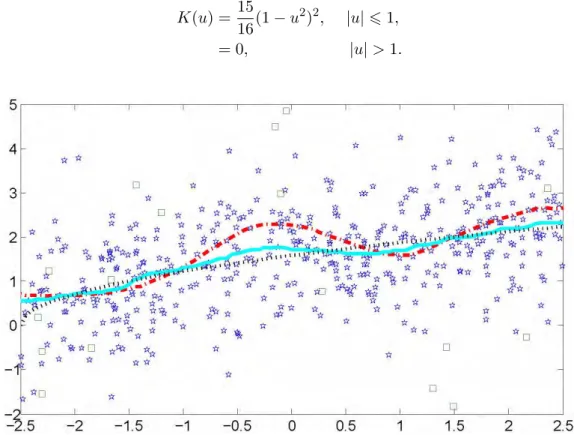
Figure 1.1: The 0.5-quantile curve, the Nadaraya-Watson estimatorm∗_n(x), and the 0. 5-quantile smootherln(x).

In Fig. 1.1 the raw data, together with the 0.5-quantile curve, are displayed. The random variables generated with probability ₁₀1 from the fat-tailed pdf 1₉ϕ(u/9), see (1.19), are marked as squares whereas the standard normal rv’s are shown as stars. We then compute both the Nadaraya-Watson estimatorm∗_n(x) and the 0.5-quantile smoother

(20)

ln(x). The bandwidth is set to 1.25 which is equivalent to 0.25 after rescalingx to [0,1]

and fulfills the requirements of Theorem 1.2.2.

In Fig. 1.1 l(x), m∗_n(x) and ln(x) are shown as a dotted line, dashed-dot line, and

solid line respectively. At first sight m∗_n(x) has clearly more variation and has the expected sensitivity to the fat-tails off(x, y). A closer look reveals thatm∗_n(x) forx≈0 apparently even leaves the 0.5-quantile curve. It may be surprising that this happens atx ≈0 where no outlier is placed, but a closer look at Fig. 1.1 shows that the large negative data values at bothx≈ −0.1 andx≈0.25 cause the problem. This data value is inside the window (h = 1.10) and therefore distorts m∗_n(x) for x ≈ 0. The quantile-smootherln(x) (solid line) is unaffected and stays fairly close to the 0.5-quantile curve.

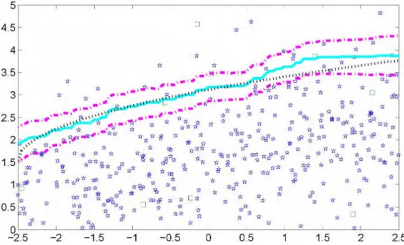
Similar results can be obtained in Fig. 1.2 corresponding to the 0.9 quantile (h = 1.25) with the 95% confidence band.

Figure 1.2: The 0.9-quantile curve, the 0.9-quantile smoother and 95% confidence band.

1.4 Application

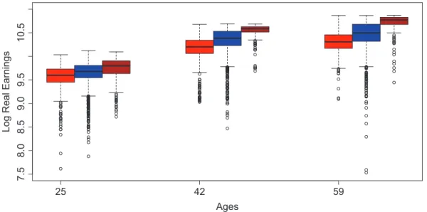
Recently there has been great interest in finding out how the financial returns of a job depend on the age of the employee. We use the Current Population Survey (CPS) data from 2005 for the following group: male aged 25−59, full-time employed, and college graduate containing 16,731 observations, for the age-earning estimation. As is usual for wage data, a log transformation to hourly real wages (unit: US dollar) is carried out first. In the CPS all ages (25 ∼ 59) are reported as integers. We rescaled them into [0,1] by dividing 40 by bandwidth 0.059 for nonparametric quantile-smoothers. This is equivalent to set bandwidth 2 for the original age data.

(21)

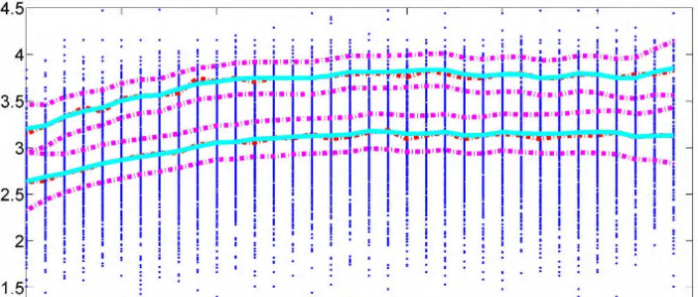
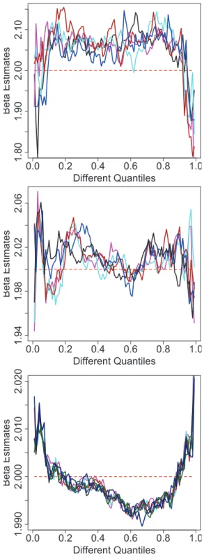
1.5 Appendix In Fig. 1.3 the original observations are displayed as small stars. The local 0.5 and 0.9 quantiles at the integer points of age are shown as dashed lines, whereas the corre-sponding nonparametric quantile-smoothers are displayed as solid lines with correspond-ing 95% uniform confidence bands shown as dashed-dot lines. A closer look reveals a quadratic relation between age and logged hourly real wages. If we use several popular parametric methods to estimate the 0.5 and 0.9 conditional quantiles, e.g. quadratic, quartic and set of dummies (a dummy variable for each 5-year age group) models as in Fig. 1.4. With the help of the 95% uniform confidence bands, we can do the parametric model specification test. At the 5% significance level, we could not reject any model. However, when the confidence level further decreases and the uniform confidence bands get narrower, “set of dummies" parametric model will be the first one to be rejected. At the 10% significance level, the set of dummies (for age groups) model is rejected while the other two are not. As the quadratic model performs quite similar by the quartic one, for simplicity, it is suggested in practice to measure the log(wage)-earing relation which coincides with Murphy and Welch (1990) in mean regression.

Figure 1.3: The original observations, local quantiles, 0.5, 0.9-quantile smoothers and corresponding 95% confidence bands.

1.5 Appendix

Proof of Theorem 1.2.1. By the definition of ln(x) as a zero of (1.2), we have, for

ε >0, ifln(x)> l(x) +ε,and thenHe_n{l(x) +ε, x}>0. (1.20) Now e Hn{l(x) +ε, x}6He{l(x) +ε, x}+ sup θ∈I |He_n(θ, x)−He(θ, x)|. (1.21)

Also, by the identityHe{l(x), x} = 0, the function He{l(x) +ε, x} is not positive and

has a magnitude _> m1qε˜ by assumption (A6) and (1.6), for 0 < ε < δ1. That is, for 0< ε < δ1,

(22)

Figure 1.4: Quadratic, quartic, set of dummies (for age groups) estimates, 0.5, 0. 9-quantile smoothers and their corresponding 95% confidence bands.

e

H{l(x) +ε, x}₆−m1qε.˜ (1.22) Combining (1.20), (1.21) and (1.22), we have, for 0< ε < δ1:

ifln(x)> l(x) +ε,and then sup θ∈I

sup

x∈J

|He_n(θ, x)−He(θ, x)|> m₁qε.˜

With a similar inequality proved for the caseln(x)< l(x)+ε, we obtain, for 0< ε < δ1:

if sup

x∈J

|ln(x)−l(x)|> ε,and then sup θ∈I

sup

x∈J

|He_n(θ, x)−He(θ, x)|> m₁qε.˜ (1.23)

It readily follows that (1.23), and (1.5) imply (1.7).

Below we first show thatkRnk∞= supt∈J|Rn(t)|vanishes asymptotically faster than

the rate (nhlogn)−1/2; for simplicity we will just use k · kto indicate the sup-norm.

LEMMA 1.5.1 For the remainder term Rn(t) defined in (1.9) we have

(23)

1.5 Appendix

Proof First we have by the positivity of the kernelK,

kRnk6 h inf 06t61{|Dn(t)| ·q(t)} i−1 {kHnk · kq−Dnk+kDnk · k EHnk} +C1· kln−lk2· n inf 06t61|Dn(t)| o−1 · kfnk∞, where fn(x) = (nh)−1Pin=1K{(x−Xi)/h}.

The desired result (1.5.1) will then follow if we prove

kHnk=Op{(nh)−1/2(logn)1/2} (1.25) kq−Dnk=Op{(nh)−1/4(logn)−1/2} (1.26)

k EHnk=O(h2) (1.27)

kln−lk2 =Op{(nh)−1/2(logn)−1/2} (1.28)

Since (1.27) follows from the well-known bias calculation EHn(t) =h−1

Z

K{(t−u)/h} E[ψ{y−l(t)}|X=u]fX(u)du=O(h2),

where O(h2_{) is independent of} _t_{in Parzen (1962), we have from assumption (}_A_{2) that}

k EHnk=Op{(nh)−1/2(logn)−1/2}.

According to LemmaA.3 in Franke and Mwita (2003), sup

t∈J

|Hn(t)− EHn(t)|=O{(nh)−1/2(logn)1/2}.

and the following inequality

kHnk6kHn− EHnk+k EHnk.

=O{(nh)−1/2(logn)1/2}+O_p{(nh)−1/2(logn)−1/2}

=O{(nh)−1/2(logn)1/2}

Statement (1.25) thus is obtained.

Statement (1.26) follows in the same way as (1.25) using assumption (A2) and the Lipschitz continuity properties of K,ψ0,l.

According to the uniform consistency ofln(t)−l(t) shown before, we have kln−lk=Op{(nh)−1/2(logn)1/2}

which implies (1.28).

Now the assertion of the lemma follows, since by tightness ofDn(t), inf06t61|Dn(t)|>

q0a.s. and thus

(24)

Finally, by Theorem 3.1 of Bickel and Rosenblatt (1973),kfnk=Op(1); thus the desired

resultkRnk=Op{(nhlogn)−1/2} follows.

We now begin with the subsequent approximations of the processes Y0,n toY5,n.

LEMMA 1.5.2

kY0,n−Y1,nk=O{(nh)−1/2(logn)2} a.s.

Proof Lettbe fixed and putL(y) =ψ{y−l(t)}still depending on t. Using integration

by parts, we obtain Z Z Γn L(y)K{(t−x)/h}dZn(x, y) = Z A u=−A Z an y=−an L(y)K(u)dZn(t−h·u, y) =− Z A −A Z an −an Zn(t−h·u, y)d{L(y)K(u)} +L(an)(an) Z A −A Zn(t−h·u, an)dK(u) −L(−an)(−an) Z A −A Zn(t−h·u,−an)dK(u) +K(A)n Z an −an Zn(t−h·A, y)dL(y) +L(an)(an)Zna(t−h·A, an)−L(−an)(−an)Zn(t−h·A,−an) o −K(−A)n Z an −an Zn(t+h·A, y)dL(y) +L(an)(an)Zn(t+h·A, an) −L(−an)(−an)Zn(t+h·A,−an) o .

If we apply the same operation to Y1,n with Bn{T(x, y)} instead of Zn(x, y) and use

Lemma 1.2.2, we finally obtain sup

06t61

h1/2g(t)1/2|Y0,n(t)−Y1,n(t)|=O{n−1/2(logn)2} a.s..

LEMMA 1.5.3 kY1,n−Y2,nk=Op(h1/2).

Proof Note that the Jacobian ofT(x, y) isf(x, y). Hence

Y1,n(t)−Y2,n(t) = {g(t)h} −1/2Z Z Γn ψ{y−l(t)}K{(t−x)/h}f(x, y)dxdy · |Wn(1,1)|.

(25)

1.5 Appendix It follows that h−1/2kY1,n−Y2,nk6|Wn(1,1)| · kg−1/2k · sup 06t61 h−1 Z Z Γn |ψ{y−l(t)}K{(t−x)/h}|f(x, y)dxdy. Since kg−1/2k is bounded by assumption, we have

h−1/2kY1,n−Y2,nk6|Wn(1,1)| ·C4·h−1

Z

K{(t−x)/h}dx=Op(1).

LEMMA 1.5.4 kY2,n−Y3,nk=Op(h1/2).

Proof The difference|Y2,n(t)−Y3,n(t)|may be written as

{g(t)h} −1/2Z Z Γn [ψ{y−l(t)} −ψ{y−l(x)}]K{(t−x)/h}dWn{T(x, y)} .

If we use the fact that l is uniformly continuous, this is smaller than h−1/2|g(t)|−1/2_{· O}

p(h)

and the lemma thus follows.

LEMMA 1.5.5 kY4,n−Y5,nk=Op(h1/2). Proof |Y4,n(t)−Y5,n(t)|=h−1/2 Z _hn_g₍_x₎ g(t) o1/2 −1iK{(t−x)/h}dW(x) 6h−1/2 Z A −A W(t−hu) ∂ ∂u hng(t−hu) g(t) o1/2 −1iK(u)du +h−1/2 K(A)W(t−hA) hng(t−Ah) g(t) o1/2 −1i +h−1/2 K(−A)W(t+hA) hng(t+Ah) g(t) o1/2 −1i S1,n(t) +S2,n(t) +S3,n(t), say.

The second term can be estimated by h−1/2kS2,nk6K(A)· sup 06t61 |W(t−Ah)| · sup 06t61 h−1 hng(t−Ah) g(t) o1/2 −1i ;

(26)

1 Confidence Bands in Quantile Regression by the mean value theorem it follows that

h−1/2kS2,nk=Op(1).

The first termS1,n is estimated as

h−1/2S1,n(t) = h −1Z A −A W(t−uh)K0(u)hng(t−uh) g(t) o1/2 −1idu 1 2 Z A −A W(t−uh)K(u)ng(t−uh) g(t) o1/2ng0(t−uh) g(t) o du =|T1,n(t)−T2,n(t)|, say; kT2,nk 6 C5 ·R−AA|W(t−hu)|du =Op(1) by assumption on g(t) = σ2(t)·fX(t). To

estimateT1,n we again use the mean value theorem to conclude that

sup 06t61 h−1 ng(t−uh) g(t) o1/2 −1 < C6· |u|; hence kT1,nk6C6· sup 06t61 Z A −A |W(t−hu)|K0(u)u/du=Op(1).

SinceS3,n(t) is estimated asS2,n(t), we finally obtain the desired result.

The next lemma shows that the truncation introduced through {an} does not affect

the limiting distribution.

LEMMA 1.5.6 kYn−Y0,nk=Op{(logn)−1/2}.

Proof We shall only show thatg0(t)−1/2h−1/2RR

R−Γnψ{y−l(t)}K{(t−x)/h}dZn(x, y)

fulfills the lemma. The replacement of g0(t) by g(t) may be proved as in Lemma A.4 of Johnston (1982). The quantity above is less than h−1/2kg−1/2k · kRR

{|y|>an}ψ{y− l(·)}K{(· −x)/h}dZ(x, y)k. It remains to be shown that the last factor tends to zero at a rateOp{(logn)−1/2}.We show first that

Vn(t) = (logn)1/2h−1/2 Z Z {|y|>an} ψ{y−l(t)}K{(t−x)/h}dZn(x, y) p →0 for all t

(27)

1.5 Appendix and then we show tightness ofVn(t), the result then follows:

Vn(t) = (logn)1/2(nh)−1/2 n X i=1 [ψ{Yi−l(t)}1(|Yi|> an)K{(t−Xi)/h} − Eψ{Yi−l(t)}1(|Yi|> an)K{(t−Xi)/h}] = n X i=1 Xn,t(t),

where {Xn,t(t)}ni=1 are i.i.d. for each n with EXn,t(t) = 0 for all t ∈ [0,1]. We then

have EX_n,t2 (t)₆(logn)(nh)−1 Eψ2{Yi−l(t)}1(|Yi|> an)K2{(t−Xi)/h} 6 sup −A6u6A K2(u)·(logn)(nh)−1 Eψ2{Yi−l(t)}1(|Yi|> an); hence Var{Vn(t)}= E n_Xn i=1 Xn,t(t) o2 =n· EX_n,t2 (t) 6 sup −A6u6A K2(u)h−1(logn) Z {|y|>an} fy(y)dy·Mψ.

whereMψ denotes an upper bound forψ2. This term tends to zero by assumption (A3).

Thus by Markov’s inequality we conclude that

Vn(t) p

→0 for allt∈[0,1].

To prove tightness of{Vn(t)}we refer again to the following moment condition as stated

in Lemma 1.5.1:

E{|Vn(t)−Vn(t1)| · |Vn(t2)−Vn(t)|}6C0·(t2−t1)2 C0 denoting a constant, t∈[t1, t2].

We again estimate the left-hand side by Schwarz’s inequality and estimate each factor separately, E{Vn(t)−Vn(t1)}2 = (logn)(nh)−1 E h_Xn i=1 Ψn(t, t1, Xi, Yi)·1(|Yi|> an) − E{Ψ_n(t, t1, Xi, Yi)·1(|Yi|> an)} i2 , where Ψn(t, t1, Xi, Yi) = ψ{Yi −l(t)}K{(t−Xi)/h} −ψ{Yi −l(t1)}K{(t1 −X1)/h}. Since ψ, K are Lipschitz continuous except at one point and the expectation is taken

(28)

1 Confidence Bands in Quantile Regression afterwards, it follows that

[E{Vn(t)−Vn(t1)}2]1/2 6C7·(logn)1/2h−3/2|t−t1| · nZ {|y|>an} fy(y)dy o1/2 .

If we apply the same estimation to Vn(t2)−Vn(t1) we finally have E{|Vn(t)−Vn(t1)| · |Vn(t2)−Vn(t)|} 6C₇2(logn)h−3|t−t1||t2−t| × Z {|y|>an} fy(y)dy 6C0· |t2−t1|2 sincet∈[t1, t2] by (A3). LEMMA 1.5.7 Let λ(K) =R

K2(u)duand let {dn} be as in the theorem. Then

(2δlogn)1/2[kY3,nk/{λ(K)}1/2−dn]

has the same asymptotic distribution as

(2δlogn)1/2[kY4,nk/{λ(K)}1/2−dn].

Proof Y3,n(t) is a Gaussian process with

EY3,n(t) = 0

and covariance function

r3(t1, t2) = EY3,n(t1)Y3,n(t2) ={g(t1)g(t2)}−1/2h−1 Z Z Γn ψ2{y−l(x)}K{(t1−x)/h} ×K{(t2−x)/h}f(x, y)dxdy ={g(t1)g(t2)}−1/2h−1 Z Z Γn ψ2{y−l(x)}f(y|x)dyK{(t1−x)/h} ×K{(t2−x)/h}fX(x)dx ={g(t1)g(t2)}−1/2h−1 Z g(x)K{(t1−x)/h}K{(t2−x)/h}dx =r4(t1, t2)

wherer4(t1, t2) is the covariance function of the Gaussian process Y4,n(t), which proves

(29)

2 Partial Linear Quantile Regression and

Bootstrap Confidence Bands

2.1 Introduction

Quantile regression, as first introduced by Koenker and Bassett (1978), is “gradually developing into a comprehensive strategy for completing the regression prediction” as claimed by Koenker and Hallock (2001). Quantile smoothing is an effective method to estimate quantile curves in a flexible nonparametric way. Since this technique makes no structural assumptions on the underlying curve, it is very important to have a device for understanding when observed features are significant and deciding between functional forms, for example a question often asked in this context is whether or not an observed peak or valley is actually a feature of the underlying regression function or is only an artifact of the observational noise. For such issues, confidence intervals should be used that are simultaneous (i.e., uniform over location) in nature. Moreover, uniform confidence bands give an idea about the global variability of the estimate.

In the previous work the theoretical focus has mainly been on obtaining consistency and asymptotic normality of the quantile smoother, thereby providing the necessary ingredients to construct its pointwise confidence intervals. This, however, is not sufficient to get an idea about the global variability of the estimate, neither can it be used to correctly answer questions about the curve’s shape, which contains the lack of fit test as an immediate application. This motivates us to construct the confidence bands. To this end, Härdle and Song (2010) used strong approximations of the empirical process and extreme value theory. However, the very poor convergence rate of extremes of a sequence of n independent normal random variables is well documented and was first noticed and investigated by Fisher and Tippett (1928), and discussed in greater detail by Hall (1991). In the latter thesis it was shown that the rate of the convergence to its limit (the suprema of a stationary Gaussian process) can be no faster than (logn)−1. For example, the supremum of a nonparametric quantile estimate can converge to its limit no faster than (logn)−1. These results may make extreme value approximation of the distributions of suprema somewhat doubtful, for example in the context of the uniform confidence band construction for a nonparametric quantile estimate.

This thesis proposes and analyzes a method of obtaining any number of uniform con-fidence bands for quantile estimates. The method is simple to implement, does not rely on the evaluation of quantities which appear in asymptotic distributions and also takes the bias properly into account (at least asymptotically). More importantly, we show that the bootstrap approximation to the distribution of the supremum of a quantile estimate is accurate to within n−2/5 which represents a significant improvement relative

(30)

2 Partial Linear Quantile Regression and Bootstrap Confidence Bands

to (logn)−1_{. Previous research by Hahn (1995) showed consistency of a bootstrap} ap-proximation to the cumulative density function (cdf) without assuming independence of the error and regressor terms. Horowitz (1998) showed bootstrap methods for median regression models based on a smoothed least-absolute-deviations (SLAD) estimate.

Let (X1, Y1), (X2, Y2), . . ., (Xn, Yn) be a sequence of independent identically

dis-tributed bivariate random variables with joint pdff(x, y), joint cdfF(x, y), conditional pdf f(y|x), f(x|y), conditional cdf F(y|x), F(x|y) for Y given X and X given Y re-spectively, and marginal pdf fX(x) for X, fY(y) for Y. With some abuse of notation

we use the letters f and F to denote different pdf’s and cdf’s respectively. The exact distribution will be clear from the context. At the first stage we assume that x ∈ J∗, and J∗ = (a, b) for some 0 < a < b < 1. Let l(x) denote the p-quantile curve, i.e. l(x) =F_Y−_|1_x(p).

In economics, discrete or categorial regressors are very common. An example is from labour market analyse where one tries to find out how revenues depend on the age of the employee (for different education levels, labour union status, genders and nationalities), i.e. in econometric analysis one targets for the differential effects. For example, Buchin-sky (1995) examined the U.S. wage structure by quantile regression techniques. This motivates the extension to multivariate covariables by partial linear modelling (PLM). This is convenient especially when we have categorial elements of theX vector. Partial linear models, which were first considered by Green and Yandell (1985), Denby (1986), Speckman (1988) and Robinson (1988), are gradually developing into a class of commonly used and studied semiparametric regression models, which can retain the flexibility of nonparametric models and ease the interpretation of linear regression models while avoid-ing the “curse of dimensionality”. Recently Liang and Li (2009) used penalised quantile regression for variable selection of partially linear models with measurement errors.

In this thesis, we propose an extension of the quantile regression model tox= (u, v)>∈

Rd with u ∈ Rd−1 and v ∈ J∗ ⊂ R. The quantile regression curve we consider is:

˜_l₍_x_{) =}_F−1

Y|x(p) =u

>_β₊_l₍_v_{). The multivariate confidence band can now be constructed,}

based on the univariate uniform confidence band, plus the estimated linear part which we will prove is more accurately (√nconsistency) estimated. This makes various tasks in economics, e.g. labour market differential effect investigation, multivariate model specification tests and the investigation of the distribution of income and wealth across regions, countries or the distribution across households possible. Additionally, since the natural link between quantile and expectile regression was developed by Newey and Powell (1987), we can further extend our result into expectile regression for various tasks, e.g. demography risk research or expectile-based Value at Risk (EVAR) as in Kuan et al. (2009). For high-dimensional modelling, Belloni and Chernozhukov (2009) recently investigated high-dimensional sparse models withL1penalty (LASSO). Additionally, by simple calculations, our result can be further extended to intersection bounds (one side confidence bands), which is similar to Chernozhukov et al. (2009).

The rest of this article is organised as follows. To keep the main idea transparent, we start with Subsection 2.2, as an introduction to the more complicated situation, the bootstrap approximation rate for the uniform confidence band (univariate case) in quan-tile regression is presented through a coupling argument. An extension to multivariate

(31)

2.2 Bootstrap confidence bands in the univariate case covariance X with partial linear modelling is shown in Subsection 2.3 with the actual type of confidence bands and their properties. In Subsection 2.4, in the Monte Carlo study we compare the bootstrap uniform confidence band with the one based on the asymptotic theory and investigate the behaviour of partial linear estimates with the corresponding confidence band. In Subsection 2.5, an application considers the labour market differential effect. The discussion is restricted to the semiparametric extension. We do not discuss the general nonparametric regression. We conjecture that this ex-tension is possible under appropriate conditions. All proofs are sketched in Subsection 2.6.

2.2 Bootstrap confidence bands in the univariate case

Suppose Yi = l(Xi) +εi, i = 1, . . . , n, where εi has distribution function F(·|Xi). For

simplicity, but without any loss of generality, we assume that F(0|Xi) = p. F(ξ|x) is

smooth as a function ofxand ξ for anyx, and for anyξ in the neighbourhood of 0. We assume:

1. X1, . . . , Xn are an i.i.d.sample, and infxfX(x) = λ0 > 0. The quantile function satisfies: sup_x|l(j)₍_x₎_{| ≤}_λ

j <∞, j= 1,2.

2. The distribution ofY givenX has a density and inf_x,tf(t|x)≥λ3 >0, continuous at all x ∈ J∗, and at t only in a neighbourhood of 0. More exactly, we have the following Taylor expansion, for someA(·) and f0(·), and for every x, x0, t:

F(t|x0) =p+f0(x)t+A(x)(x0−x) +R(t, x0;x), (2.1) where sup t,x,x0 |R(t, x0;x)| t2₊_|_x0₋_x_|2 <∞.

Let K be a symmetric density function with compact support anddK =R u2K(u)du < ∞. Letlh(·) =ln,h(·) be the nonparametricp-quantile estimate ofY1, . . . , Ynwith weight

functionK{(Xi− ·)/h} for some global bandwidthh=hn (Kh(u) =h−1K(u/h)), that

is, a solution of:

Pn i=1Kh(x−Xi)1{Yi < lh(x)} Pn i=1Kh(x−Xi) < p≤ Pn i=1Kh(x−Xi)1{Yi ≤lh(x)} Pn i=1Kh(x−Xi) . (2.2) Generally, the bandwidth may also depend onx. A local (adaptive) bandwidth selection though deserves future research.

Note that by assumption (A1),lh(x) is the quantile of a discrete distribution, which

is equivalent to a sample of sizeO_p(nh) from a distribution withp-quantile whose bias is

O(h2_{) relative to the true value. Let}_δ

n be the local rate of convergence of the function

lh, essentially δn=h2+ (nh)−1/2=O(n−2/5) with optimal bandwidth choice h=hn= O(n−1/5). We employ also an auxiliary estimate lg

def

(32)

2 Partial Linear Quantile Regression and Bootstrap Confidence Bands

ln,h but with a slightly larger bandwidth g = gn = hnnζ (a heuristic explanation of

why it is essential to oversmoothg is given later), where ζ is some small number. The asymptotically optimal choice ofζ as shown later is 4/45.

3. The estimatelg satisfies:

sup x∈J∗ |l00_g(x)−l00(x)|=O_p(1), sup x∈J∗ |l0_g(x)−l0(x)|=O_p(δn/h). (2.3)

Assumption ( A3) is only stated to overwrite the issue here. It actually follows from the assumptions on (g, h). A sequence {an} is slowly varying if n−αan → 0 for any α >0.

With some abuse of notation we will useSnto denoteanyslowly varying function which

may change from place to place e.g. S_n2 =Sn is a valid expression (since ifSnis a slowly

varying function, then S_n2 is slowly varying as well). λi and Ci are generic constants

throughout this thesis and the subscripts have no specific meaning. Note that there is no Sn term in (2.3) exactly because the bandwidth gn used to calculate lg is slightly

larger than that used for lh. We want to smooth it such that,lg, as an estimate of the

quantile function, has a slightly worse rate of convergence, but its derivatives converge faster.

We also consider a family of estimates ˆF(·|Xi), i= 1, . . . , n, estimating respectively

F(·|Xi) and satisfying ˆF(0|Xi) = p. For example we can take the distribution with a

point massc−1K{αn(Xj−Xi)}onYj−lh(Xi),j = 1, . . . , n, wherec=Pnj=1K{αn(Xj−

Xi)}and αn≈h−1, i.e. ˆ F(·|Xi) = Pn j=1Kh(Xj−Xi)1{Yj−lh(Xi)≤ ·} Pn j=1Kh(Xj −Xi) We additionally assume:

4. fX(x) is twice continuously differentiable andf(t|x) is uniformly bounded inxand

t by, say,λ4.

LEMMA 2.2.1 [Franke and Mwita (2003), p14] If assumptions (A1, A2, A4) hold,

then for any small enough (positive)ε→0, sup

|t|<ε,i=1,...,n,Xi∈J∗

|Fˆ(t|Xi)−F(t|Xi)|=Op{Snδnε1/2+ε2}. (2.4)

Note that the result in Lemma 2.2.1 is natural, since by definition, there is no error at t = 0, since ˆF(0|Xi) ≡ p ≡ F(0|Xi). For t ∈ (0, ε), ˆF(t|Xi), like lh, is based on a

sample of size Op(nh). Hence, the random error is Op{(nh)−1/2t1/2}, while the bias is O_p(εh2) =O_p(δn). The Sn term takes care of the maximisation.

LetF−1(·|·) and ˆF−1(·|·) be the inverse function of the conditional cdf and its estimate. We consider the following bootstrap procedure: Let U1, . . . , Un be i.i.d.uniform [0,1]

variables. Let

(33)

2.2 Bootstrap confidence bands in the univariate case be the bootstrap sample. We couple this sample to an unobserved hypothetical sample from the true conditional distribution:

Y_i#=l(Xi) +F−1(Ui|Xi), i= 1, . . . , n. (2.6)

Note that the vectors (Y1, . . . , Yn) and (Y1#, . . . , Yn#) are equally distributed given

X1, . . . , Xn. We are really interested in the exact values of Yi# and Yi∗ only when they

are near the appropriate quantile, that is, only if|Ui−p|< Snδn. But then, by equation

(2.1), Lemma 2.2.1 and the inverse function theorem, we have: max i:|F−1₍_U i|Xi)−F−1(p)|<Snδn |F−1(Ui|Xi)−Fb−1(U_i|X_i)| = max i:|Y_i#−l(Xi)|<Snδn |Y_i#−l(Xi)−Yi∗+lg(Xi)|=Op{Snδn3/2}. (2.7)

Let now qhi(Y1, . . . , Yn) be the solution of the local quantile as given by (2.2) at Xi,

with bandwidthh, i.e. qhi(Y1, . . . , Yn)

def

= lh(Xi) for data set{(Xi, Yi)}ni=1. Note that by (2.3), if |Xi−Xj|=O(h), then

max

|Xi−Xj|<ch

|lg(Xi)−lg(Xj)−l(Xi) +l(Xj)|=Op(δn) (2.8)

Let l_h∗ and l#_h be the local bootstrap quantile and its coupled sample analogue. Then l∗_h(Xi)−lg(Xi) =qhi[{Yj∗−lg(Xi)}nj=1]

=qhi[{Yj∗−lg(Xj) +lg(Xj)−lg(Xi)})nj=1], (2.9) while

l#_h(Xi)−l(Xi) =qhi[{Yj#−l(Xj) +l(Xj)−l(Xi)}nj=1]. (2.10) From (2.7) – (2.10) we conclude that

max

i |l

∗

h(Xi)−lg(Xi)−l#h(Xi) +l(Xi)|=Op(δn). (2.11)

Based on (2.11), we obtain the following theorem (the proof is given in the appendix):

THEOREM 2.2.1 If assumptions (A1 - A4) hold, then

sup

x∈J∗

|l∗_h(x)−lg(x)−lh#(x) +l(x)|=Op(δn) =Op(n−2/5).

A number of replications of l_h∗(x) can be used as the basis for simultaneous error bars because the distribution of l#_h(x) −l(x) is approximated by the distribution of l∗_h(x)−lg(x), as Theorem 2.2.1 shows.

Although Theorem 2.2.1 is stated with a fixed bandwidth, in practice, to take care of the heteroscedasticity effect, we construct confidence bands with the width depending on the densities, which is motivated by the counterpart based on the asymptotic theory

(34)

2 Partial Linear Quantile Regression and Bootstrap Confidence Bands as in Härdle and Song (2010). Thus we have the following corollary:

COROLLARY 2.2.1 Let d∗α be defined by P∗(|l∗_h(x)−lg(x)| > d∗α) =α), where P∗

is the bootstrap distribution conditioned on the sample. If ( A1)–( A4) hold, then the confidence intervallh(x)± d∗α has an asymptotic uniform coverage of1−α, in the sense

thatP(sup_x_∈_J∗|l_h(x)_l(x)|> d∗_α)→α.

In practice we would use the approximate (1−α)×100% confidence band over_Rgiven by lh(x)± h ˆ f{lh(x)|x} q ˆ fX(x) i−1 d∗_α,

where d∗_α is based on the bootstrap sample (defined later) and ˆf{lh(x)|x}, fˆX(x) are

consistent estimators off{l(x)|x}, fX(x) with use off(y|x) =f(x, y)/fX(x).

Below is the summary of the basic steps for the bootstrap procedure:

1) Given (Xi, Yi), i= 1, . . . , n, compute the local quantile smootherlh(x) ofY1, . . . , Yn

with bandwidth hand obtain residuals ˆεi =Yi−lh(Xi), i= 1, . . . , n.

2) Compute the conditional edf: ˆ F(t|x) = Pn i=1Kh(x−Xi)1{εˆi 6t} Pn i=1Kh(x−Xi)

3) For each i = 1, . . . , n, generate random variables ε∗_i,b ∼Fˆ(t|x), b = 1, . . . , B and construct the bootstrap sample Y_i,b∗, i= 1, . . . , n, b= 1, . . . , B as follows: