Bancarizing with Credit Cards: Experimental Evidence on Interest Rates and Minimum Payments Elasticities for New Clients

(1)

Banco de México

Documentos de Investigación

Banco de México

Working Papers

N° 2015-11

B a n c a r i z i n g w i t h C r e d i t C a r d s : E x p e r i m e n t a l E v i d e n c e

o n I n t e r e s t R a t e s a n d M i n i m u m P a y m e n t s E l a s t i c i t i e s

f o r N e w C l i e n t s

June 2015

La serie de Documentos de Investigación del Banco de México divulga resultados preliminares de trabajos de investigación económica realizados en el Banco de México con la finalidad de propiciar el intercambio y debate de ideas. El contenido de los Documentos de Investigación, así como las conclusiones que de ellos se derivan, son responsabilidad exclusiva de los autores y no reflejan necesariamente las del Banco de México.

The Working Papers series of Banco de México disseminates preliminary results of economic research conducted at Banco de México in order to promote the exchange and debate of ideas. The views and conclusions presented in the Working Papers are exclusively the responsibility of the authors and do not necessarily reflect those of Banco de México.

E n r i q u e S e i r a

ITAM - Banco de México

S a r a G . C a s t e l l a n o s

Banco de México

D i e g o J . J i m é n e z H e r n á n d e z

(2)

B a n c a r i z i n g w i t h C r e d i t C a r d s : E x p e r i m e n t a l E v i d e n c e o n

I n t e r e s t R a t e s a n d M i n i m u m P a y m e n t s E l a s t i c i t i e s f o r

N e w C l i e n t s

*

Abstract: We study the bancarization of marginal borrowers using credit cards and document that this process is difficult: default risk is substantial, returns heterogeneous, and account closings common. We also take advantage of a randomized control trial that varied interest rates and minimum payments in a very wide range. Against our hypothesis, we find that default risk is very insensitive to (randomized) large changes in interest rates and minimum payments. This could imply that regulating these contract terms may not necessarily "protect" consumers against default and that moral hazard in this market is negligible on average.

Keywords: Credit cards, Development finance, Consumer behavior, Mexico.

JEL Classification: D14, D18, D82, G21

Resumen: Se estudia la bancarización de los consumidores marginales por medio de tarjetas de crédito y se documenta que dicho proceso es difícil: el riesgo de impago es alto, los retornos son heterogéneos y el cierre de cuentas es común. Además, se utiliza un experimento aleatorio que varió tasas de interés y pagos mínimos en un rango muy amplio. Contrario a nuestra hipótesis, se encuentra que el riesgo de impago es muy insensible a grandes cambios (aleatorios) en la tasa de interés y en el pago mínimo. Esto podría implicar que regular dichos términos del contrato quizás no necesariamente "protege" a los consumidores contra impago y que el riesgo moral en este mercado es negligible en promedio.

Palabras Clave: Tarjetas de crédito, Finanzas en mercados en desarrollo, Comportamiento del consumidor, México Documento de Investigación 2015-11 Working Paper 2015-11

E n r i q u e S e i r a

y

S a r a G . C a s t e l l a n o s

z

Banco de México

D i e g o J . J i m é n e z H e r n á n d e z

x

*We thank Ana Aguilar and Alan Elizondo for the support in this project. We also thank Eduardo Laguna for his valuable research assistance.

y Centro de Investigación Económica (ITAM) and Dirección General de Investigación Económica (Banco de

(3)

1 Introduction

Incorporating marginal borrowers into formal banking is both important and diﬃcult.

It is important since it may relax borrowing constraints and help mobilize savings across

a larger scope of projects. It is diﬃcult because borrower risk and the optimal level of

parameters like interest rates, credit sizes, and minimum payments have to be learned

along the way. In developing countries it is especially diﬃcult to give loans to new

borrowers which lack a credit history since the frameworks to recover collateral rarely

function eﬀectively1_.

Credit cards oﬀer a way to mitigate these diﬃculties to some extent. First, credit

cards are designed to require no collateral. Second, the bank learns fast about the borrower type since the borrower conveys information with high frequency and this in-formation is used to update the credit line. Indeed, in Mexico bancarization of marginal

borrowers is happening mainly through the award of credit cards. Figure 1shows that

the number of credit cards in Mexico was growing rapidly until 2008 when the global

cri-sis hit. The non-performing credit cards portfolio also increased. Figure2ashows that

the expansion of credit cards in 2004-2010 was concentrated in the lower three deciles

of income, whereas2bshows that a very important point of entry into the formal credit

market in Mexico is through credit cards, with over 60% of all new entries.2

The increase in non-performing loans is the natural outcome of incorporating new

marginal borrowers. Banks and authorities are interested in how financial diﬃculties

and eventual default can be mitigated by contract design, in our case interest rates and minimum payments. This concern is also present in the US for instance. Worried that the minimum payment was too low, the US congress required a study of minimum payments in cards in the early 2000s (Smale 2005). The study found that minimum payment requirements had decreased markedly over time: in the 1970s the average card minimum payment was about 5% of the outstanding balance, and by 2000 it was down to 2%. In January 2003, US Federal regulators jointly issued interagency guidance on credit card lending, among other things it stated that minimum payments are too low and pressured for their increase. Nevertheless, theoretically it is no obvious what is meant by “too low”.

The aftermath of the financial crisis of 2008 has only increased these concerns, with 1_{Karlan & Zinman (2008) report default rates twice as big for new borrowers of a micro-finance}

institution in South Africa for instance.

2_{This sample was taken from the credit bureau, conditioning on people who had a credit card. So}

(4)

authorities placing credit cards under the magnifying glass. Canada, Mexico and the US have enacted legislation in this respect. The US adopted the CARD Act in 2009, Canada adopted the New Credit Card Rules in 2010; both pieces of legislation focus mostly on disclosure. In 2010 authorities in Mexico established a floor on the minimum

payment that credit providers can charge.3

This paper focuses on three issues: First, it provides a rare window into the bancar-ization process in a developing country by studying one such strategy in an important bank in Mexico. We show that incorporating new borrowers into the banking sector is risky as returns are very heterogeneous and many clients leave the bank/card in a short span of time. Second, we examine data from a randomized experiment with new clients to measure if changes in the interest rate and minimum payments impacted de-fault. Third, we show that even for this population with presumably high asymmetric information, there is no evidence of moral hazard/repayment burden as interest change significantly, supporting the result of Karlan & Zinman (2009).

The sample of 162,000 accounts in the paper comes from a population of clients with at least 6 months of good behavior in our bank. These clients were brought in by sales

eﬀorts of the bank in supermarket chains, a common practice in Mexico. The bank

ran an experiment with this sample and varied interest rates and minimum payments in a controlled randomized fashion. In particular the card holders were allocated to 8

diﬀerent treatments. Yearly interest rates where randomized in {45%, 35%, 25%, 15%}

and minimum payment (MP) as a percentage of debt was randomized orthogonally in {5%, 10%}. These parameters were then kept constant at these levels for 26 months between March 2007 and May 2009. No promotions were given to them during this period. After that period all consumers reverted back to normal conditions at interest rates of about 45% and minimum payments of close to 5% of debt. The size of the credit line was allowed to vary normally, according to the protocols of the risk department and independently of treatment status.

This experiment is of substantial policy interest, especially the variation in mini-mum payment which has not been studied in a randomized control trial in the literature. Although there have been discussions in the US, Canada and Mexico to increase mini-mum payments, there is no evidence of the potential implications of this. Supporters of the policy say that low minimum payment leads unsophisticated or present biased con-sumers to incur in too much debt which leads to default. Meier & Sprenger (2010) and 3_{The minimum payment has to be the maximum of 1.5% of the balance plus the amount of interest}

(5)

Laibson, Repetto & Tobacman (2003) provide some evidence consistent with present-biased preferences driving some variation in credit card borrowing, and Stewart (2009) shows that payments seem to anchor at the minimum payment. Detractors on the other hand say that consumers are not so unsophisticated and that the policy would limit

the ability of households to smooth consumption, with little eﬀect on default. We find

that for our population increasing the minimum payment substantially did not in fact lead to significantly less default, although it did decrease debt.

We find that as a percentage of their respective means, increasing the minimum payment from 5% of debt to 10% leads to an increase in payments of 13% one year later and an associated reduction in debt of 12% a year later and of 24% two years later.

So the minimum payment policydoes aﬀect leverage. However it does not aﬀect default

in an economically significant magnitude. Since the lower revenues from lower debt is

not oﬀset in a big way by reduced default –with only a 3% diﬀerence in cumulative

default as a percentage of its mean or 0.7pp overall–, the net-of-default revenue of the bank decreases by 7% in net present value.

Estimation of debt-interest elasticities is more commonly performed in the

litera-ture, although not in a setup like ours. Gross & Souleles (2002) estimate the eﬀect of

changing interest rates for credit card holders in the US. They find a long run elasticity debt in of -1.3 but do not have as clean exogenous variation as ours. Karlan & Zinman (2008) estimate elasticities take-up for micro-finance clients in short term fixed payment loans and find a relatively small elasticity of -0.28. We make three contributions to this

previous work: we use randomized variation in interest rates to identify elasticities4_{, we}

focus on new marginal borrowers5_{, and we study the intensive margin (as opposed to}

take-up) not only of debt, but also the channels of its change like purchases and pay-ments, as well as default and account closings; this latter variable could be interpreted as losing access to credit if it is closed by the bank.

To give a flavor of the results, we find that going from 45% interest rate to 15% causes purchases to increase by 9%, payments to fall by 5%. In in spite of this, debt

decreases by about 18%.6 _{Default decreases by only 6% of its mean (1pp overall) and}

revenues fall by 7%. Cancelations are only 1 percentage point higher with a 45% interest 4_{Karlan & Zinman (2008) called for more randomized experiments to measure elasticities, but few}

papers have answered this call.

5_{Those that have not had loans from banks but are in the margin of being credit worthy for banks.}

KZ focused on borrowers who had already borrowed from the lender.

6_{The positive association between debt and interest rates is partly due to compound interest,}

(6)

rate vis-a-vis the 15% interest rate.

Within the experiment, the data also reveals fast learning of risk by the issuer as reflected in credit limit increases. The strategy seems to be to award low credit limits at about 9,000 pesos on average (less than 700 usd) when the account is opened, and then increase credit limits fast – a 40% increase in the first 10 months– as the borrower pays on time and sequentially reveals to be a good risk (with its due credit risk analysis). Borrowers who miss payments are penalized with substantially lower limits.

The rest of this article is organized as follows. Section 2 describes the experiment

and the data. We present the results about minimum payment variations in Section

3 and those about interest rate variations in Section 4. Section 5 explores the role of

delinquencies and default on credit limits. Section6deals with attrition and robustness

of our findings and, finally, Section7 concludes.

2 The data and the experiment

2.1 Our sample

Our population consists of new low and medium income clients that the cooperating commercial bank (from now on called the bank) recruited in supermarket chains to have a credit card. For some of them this is their first banking product. Our sample is a stratified random sample of this population, as will be described below. The bank took a random sample from this population, with the condition that they have had at least 6 months in the bank with no default.

For the sample in this experiment we observe the following variables with a monthly frequency: interest paying debt (and therefore the amount of consumers who pay in-terests each month), debt balance at the end of the period, purchases and payments, minimum payment due, delinquencies (failing to pay the minimum payment), default (3 consecutive delinquencies), credit limit, client initiated cancelations, and all cance-lations. We also observe, for every consumer at the beginning of the experiment, the number of months of tenure with the card and a measure of payment behavior that is thoroughly explained in the following section. Finally, we observe age, gender, and marital status for about 60% of the sample.

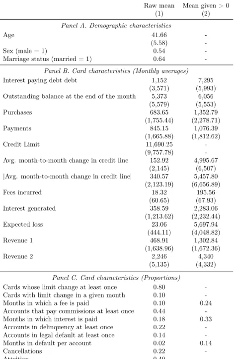
Table 1 contains the descriptive statistics of the main variables for our sample. In

particular, Panel B provides information regarding consumers at the month level. The average credit line is 11,690 pesos (less than 1,000 USD) and average debt is almost

(7)

a tenth of this at 1,152 pesos. Most borrowers are non revolvers, 18% of observations involve incurring in interest. Bank policy about the size of lines is quite active, 80% of accounts experience a limit change during our 26 month sample period. Payment and purchases are large relative to interest paying debt. There is substantial heterogeneity reflected in the standard deviations, which are about twice as large as the means. We are told that this heterogeneity is typical of pools of new borrowers which have not

undergone the natural selection process. Figure 5 shows the distribution of revenues7_,

separating across those that defaulted and those who didn’t. This just highlights that there is substantial risk in bancarization.

Repayment risk is also high, 22% of accounts missed a payment at least once and 14% accounts defaulted (more than 90 days delinquent) at least once. Net of default revenues also show substantial heterogeneity: the standard deviation of the Revenue 1 measure is 4 times the mean for instance. Finally, note that 39% of accounts leave our sample, with 21% leaving because consumers close their accounts. The Appendix presents evidence showing that quantitatively the attrition is not unbalanced across the experimental groups, both in terms of the the number of accounts that we lose and in terms of the the characteristics of those accounts. To deal with attrition we present results after one and two years separately.

2.2 The Experiment

The experiment started in March 2007. The bank provided a sample composed by 9

diﬀerent strata, which were created using 2 categorical variables with 3 values each (see

Table 2c). The categories were months of tenure with the card (6 to 12 months, 12

to 23 months, and 24 months and more), and payment behavior (full balance payer, part balance payer, minimum payment payer). Within each of these 9 strata, the bank randomly selected 18,000 accounts, so that the random sample, in total, includes

162,000 of cards. This sample was later on assigned into 8 diﬀerent treatments and one

control by randomization.

Secondly, each of these sets of 18,000 accounts were randomly allocated to 9 groups, 7_{We computed the revenue as two diﬀerent present values. Both present values are computed for}

March 2007 with a discount rate of 5 percent. Revenue 1 was computed using the present value of interest generated debt plus the bank commissions minus a rough measure of expected loss. This measure was calculated by using one half of the total amount due when the account defaulted and then attrited. Revenue 2 was computed using the present value of payments made during the sample during the sample period minus the present value of purchases made and the expected loss.

(8)

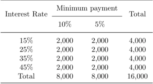
a control group of 2,000 accounts and 8 treatment groups of also 2,000 accounts each. The treatment groups are defined by the interest rate and the minimum payment rate as a proportion of debt, as follows: {interest rate, minimum payment} in {45%, 35%,

25%,15%} ⇥ {5%, 10%}, see table 2. The randomly allocated interest rate and

mini-mum payment were mandatory, became eﬀective in March 2007, and lasted until May

2009 when the experiment ended (see Figure 3 for more information).8 _{Increases in}

credit limits were not dependent on treatment status (see Table 4). Table 3 provides

evidence that randomization did balance the sample across treatment groups.

2.3 Empirical Strategy

Since treatment is randomized, we will simply estimate its causal eﬀect by the parameter

in the following equation:

Yitk =↵+

X k

kTik+✏ikt (1)

Where k measure the eﬀect of treatment k on outcome Y with respect to the

omitted group. The indexi indexes credit cards andtindexes months. We will provide

cross-sectional estimates after one year of treatment (t = 13) and at the very end of

our experiment 26 months later. We decided to use only the cross-section data in the regression for simplicity.

For dependent variables we use interest paying debt, purchases, payments, two measures of (net of default) revenue. The first measure (Revenue 1) calculates for each month interest and fee income and subtracts a rough measure of expected loss

of the account if it defaulted,9 _{it then calculates the present value using an interest}

rate of 5% for the sample period. The second measure of revenue calculates for each month payments minus purchases, since this is the net flow of income and treats the default as in Revenue 1, and again brings this to the present using a 5% rate. We also study cumulative delinquency, cumulative default and cumulative cancelations to deal with attrition. An account is delinquent in this definition when it has had at least one late payment in the sample period up to the month of consideration. An account is in 8_{In the paper we will not use the pure control group much since it is not clear exactly what their}

interest rate and minimum payment was during this period except that the former was higher than 45% and the later lower than 5%.

9_{We do not observe severity of loss so we assume is half of the outstanding balance at the time of}

(9)

default when it has had 3 consecutive months delinquent.

3 E

ﬀ

ect of variations in the minimum payment

In many countries minimum payment policy is an issue of contempt between financial authorities and banks. On one hand, bank profitability requires that clients revolve debt and pay interest as long as this debt is not defaulted upon. On the other hand however, if banks do not take into account that a larger client’s debt may induce default in other banks (externalities), or if clients have present biased preferences or are unsophisticated, then the privately optimal minimum payment set by banks does not necessarily coincide with the social optimum, the minimum payment set by policy may be too low, giving rise to higher debt and higher default then the socially optimal one. The concern is genuine given that that minimum payments in Mexico ocasionally generated negative amortization of debt in the past, giving rise to regulation in 2010 in the Circular 34/2010 from Banco de Mexico that set a floor on minimum payments.

The social welfare case for increasing minimum payment as a consumer protection device depends on whether consumers are overindebted and are at risk of default, per-haps because they have present-biased preferences or are unsophisticated. Meier & Sprenger (2010) and Laibson, Repetto & Tobacman (2003) provide evidence consistent with individuals displaying present biased preferences in the use of their credit card. But is overindebtedness so high as to impact default? And is it the case that minimum

payment policy aﬀects default as a consequence?

Our experiment suggestsit does not, at least within the range of variation we study

and for this sample of clients. The eﬀects are negligible, especially in the long run

(after 10 or so months). In the very short run a higher minimum payment does increase delinquency. This may happen if individuals do not realize that their minimum payment

increased10_{, or if they cannot immediately a}_ﬀ_{ord to pay, which is likely in our experiment}

given that minimum payment was doubled with a little advanced notice.

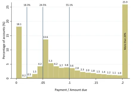
Figure 4 shows that about 25% clients paid less than 5% of debt and 56% paid

less than 10% of debt at the start of the experiment before MP policy aﬀected them.

This means that experimental minimum payment policy of 5% and 10% will bind for

a substantial fraction of clients. A higher minimum payment could aﬀect payments if

it binds and clients want to avoid fees and being reported in the credit bureau, but it 10_{The minimum payment features prominently in the monthly statement however.}

(10)

could also potentially aﬀect payment for clients for who use payment rules which use

the minimum payment as an anchor.11

Minimum payment policy can aﬀect profitability through two main channels. The

first is selection: it may be that risky clients are the ones that want more leverage, so that when the minimum payment increases they are hurt and close the account. All else constant, this may be a positive outcome for the bank as it could lead to less default and more profitability. In this way minimum payments may act as a screening

device12_{. The second channel is that a higher minimum payment may lead to lower}

debt –through more payments and/or less purchases– and thus to lower profits.

Tables 5 and 6 show the estimates of equation (1), comparing debt, purchases,

payments and revenue for the group of consumers who were assigned to pay minimum payments of 10% of debt versus those that only had to pay 5%. Panel A reports results 13 months after treatment and Panel B reports results 26 months after treatments.

Note first that increasing MP from 5% to 10% causes debt to decrease substantially.

This eﬀect, however, is not monotone across diﬀerent interest rate levels in the medium

term. By April 2008, an increase in the minimum payment decreases debt in 131, 219, 70 and 110 pesos for the cards with an interest rate of 45%, 35%, 25% and 15%,

respectively.13 _{On the long run, debt decreases when the MP increases –and it decreases}

more with in the groups with higher interest rate levels–. By May 2009, the reduction is 541, 297, 294 and 210 for the interest rates of 45%, 35%, 25% and 15%, respectively. This is a large reduction in debt of almost 25% on average after 2 years. Payments increase substantially, ranging from 128 pesos for the 15% interest rate strata to 75 pesos for the 45% interest rate group. These changes are equivalent, on average, to 12% of average payments in the 5MP group. Somewhat surprisingly purchases also increase. We don’t know how to explain this. One possibility is that paying more actually liberates credit line and allows consumers to buy more. Another possibility is that the higher MP acts as a commitment device to pay more, and anticipating this

they can aﬀord to purchase more knowing that they will have to pay oﬀ a larger share

of these purchases. All eﬀects are statistically significant.

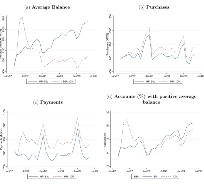
The dynamics of the eﬀect are interesting. Pooling across interest rates, Figure 6a

shows that initially there is a jump in average debt of the 10MP group. This seems to 11_{In unreported analysis we did not find evidence of minimum payments influencing those people}

who already pay much more than the minimum.

12_{See Adams, Einav & Levin (2009) for a discussion or related issues in other context.} 13_{A test for the aforementioned quantities being equal yields a p-value of 0.0509.}

(11)

be the result of the accumulation of late payment fees. By September 2007 –6 months after the start of the experiment– however debt is lower in the 10MP group. Payments,

shown in Figure 6c, also show a sudden increase, whereas in purchases the increase is

smoother.14 _{Note finally that debt trends upwards for the 5MP group accumulating}

gradually during all 2008 and 2009, whereas it is flat for the 10MP group.

In spite of inducing a large decrease in debt, the 10% minimum payment treatment

has a tiny eﬀect on default and delinquency. Interestingly enough, this eﬀect is

statisti-cally significant for the 15% and 25% percent strata, but not for the 35% and 45% ones.

There is a transitory increase in delinquency as reflected in Figure 6e. In April 2008,

Table 5 shows that whereas the 5MP strata had on average 12.2%15 _{of accounts were}

at least one month in arrears at some point, the 10MP group had and extra 2.2% –on

average– in arrears. This diﬀerence is even smaller by May 2009, only 1.2% extra out

of 22.6% for the 5MP group. Figure6gshows that as percentage of surviving accounts

there is no diﬀerence in delinquency between the two groups in May 2009.

This is telling. If bad risks self select out as a result of higher minimum payment,

the dotted line in Figure 6g should cross the solid line from above and lie below it

afterwards. This does not happen and therefore it doesn’t seem like a higher minimum payment leads to a less risky population of clients, even when debt is smaller for the 10% group. Finally cancelations are 21% for the 5MP group compared to 22% for the 10MP group. Since higher MP induces less borrowing and not less defaults, revenue

suﬀers. The decrease in net of default revenue is 7% for our Revenue 1 measure and 20%

for our Revenue 2 measure. All in all, increasing the minimum payment substantially

lower interest paying debt, but did not aﬀect default.

We found no treatment heterogeneity across demographic groups by median age, gender, marital status, and experience with the card. We did find that people that were stratified into the “pays close to the MP” category experienced larger increases in debt, purchases, payments and delinquencies than full balance payers, in pesos -586, +102, +73, +0.03pp respectively after two years, all significant at the 1% level.

14_{There is also a large seasonal component, with purchases increasing around Christmas and}

pay-ments just after that.

15_{This number can be decomposed on 11.7 (15% IR), 12 (25% IR), 12.5 (35% IR), 12.4 (45% IR)}

(12)

4 E

ﬀ

ect of interest rate variations

Estimating demand interest elasticities is necessary to determine profit maximizing prices, as well as useful for conducting welfare analysis. Banks in Mexico sometimes conduct randomized control trials to measure debt-interest elasticities.

There is also a growing literature measuring the price elasticity of demand for credit

products, but their context is quite diﬀerent from ours. Karlan & Zinman (2008, KZ)

and Dehejia, Montgomery & Morduch (2012, DMM) study take-up elasticities for micro-finance in South Africa and Bangladesh respectively. Only the former uses randomized variation in interest rates while the later use across branch price variation. DMM find elasticities between -0.7 and -1 while KZ’s elasticities are in the order of -0.28. We study

a diﬀerent product (credit cards) and focus on intensive margin responses, whereas they

study take-up. Thus our paper complements this growing literature.

Table 5 shows our estimates of responses to interest rate diﬀerences. In the long

run, the debt-interest elasticities we estimate are 0.37 for the 5MP group and 0.10 for the 10MP group. Note that they are positive. At first this may seem puzzling, but it is due to interest compounding. The fact that debt is revolving and interest accumulates explains why higher interest leads to more debt. In contrast, higher interest leads to lower purchases and higher payments. Purchase elasticities from a change of 45% interest rate to 35%, 25% and 15% interest rate respectively are 0.14, 0.01, -0.13 (measured in May 2009, pooled across minimum payments). This elasticities are somewhat low. They imply that tripling the interest rate from 15% to 45% results in a decrease of less than 10% in purchases. Payment elasticities to interest rates, pooling across minimum payments, are equally small, 0.02, 0.12, 0.08 respectively.

Consistent with this small eﬀects, the eﬀect on default is also relatively small. Take

the 10MP group and look at long term accumulated default. For this group changing the interest rate from 45% to 15% results in a 1.3pp reduction in default, from a baseline of about 22pp. The analogous numbers taking the 5MP group are a decrease in default from 21pp to 19.5pp. This is worthwhile to highlight. Large changes in interest rates

and their associated incentive and repayment burden eﬀects are not reflected in default.

In other words, we do not find evidence of moral hazard16 _{even for this population of}

new borrowers.

Our finding is consistent with Karlan & Zinman’s (2009) findings. Our results are important since their seminal and influential findings have been criticized because of

(13)

small sample size and sample composition issues. We have larger percentage variation, a sample size which is 30 times bigger, and borrowers who are not habitual borrowers from the bank (or from any bank) but truly new borrowers for which asymmetric information could be large. Note also that if anything our measure is biased towards finding more

default: since debt increases along with interest the mechanical eﬀect of larger debt

(which is harder to pay) reinforces the behavioral moral hazard eﬀect. In spite of this

we find a zero combined eﬀect.17

Small interest elasticities seem to confirm the often mentioned statement that low income consumers and/or consumers new to the formal credit sectors do not have many alternatives for borrowing, and that this makes them makes them exhibit inelastic

responses to changes in interest rates. This is also reflected in the small eﬀect on

cancelations: one percentage point lower in the 15% group from a base of 22 percentage points in the 45% group.

The variation spanned in debt, purchases and payments by varying interest rates between 15% and 45% is similar to that spanned by varying minimum payments between 5% and 10%. Note however that this is not true for (net of default) Revenue 1. Since higher interest is accompanied by higher debt increasing interest is highly profitable. Note that default and canceled accounts are only slightly higher with a 45% than with a 15% rate: 1% and 2% of extra accounts respectively. As a result revenue is almost

twice as big at 45% interest vs at 15%. The dynamics of the eﬀects are reported in

Figure 7.

5 Credit limits and learning

It is a typical bank policy in Mexico to approve very low limits when the card is first awarded and increase them as the borrower reveals to be a good risk. Einav, Jenkins & Levin (2013) have shown that quantity restrictions are used to limit risk in lending

to subprime borrowers and that they are very eﬀective.18 _{Higher limits typically lead}

to higher default, but also to higher debt and thus higher interest income. Banks solve 17_{The results are conditional on selection since few people leave because of increasing rates, allowing}

us to talk about moral hazard without being contaminated by adverse selection. On the other hand since credit cards are open-ended loans, and since interest rates were randomized downwards, keeping the card in good status has the option value of accessing cheap credit in the future, as in KZ moral hazard treatment.

18_{Their setting however is diﬀerent from ours since the quantity restriction plays an important role}

in selecting/screening applicants, whereas in our case they are selected already. Also in our context there is repeated interaction and learning.

(14)

this trade-oﬀto maximize profit, and when risk is revealed to be lower than the optimal banks respond by increasing credit limits.

We are interested in quantifying how fast is limit increased to good payers, and to what extent are bad payers awarded lower limits. To this end we estimate the following equation:

Limitit=↵i+ t+✓D(cum_delinquencies) + D(cum_def aults) +✏ijt (2)

where cum_delinquencies is a measure of cumulative defaults in the previous

months. Note that by controlling for account fixed eﬀects ↵i, the ✓ and measure

how the credit limit is decreased by the bank when a given person incurs in late

pay-ments or defaults. To control flexibly for delinquencies or defaults we use dummies for 1,2,3...,11 and more cumulative delinquencies and 1,2,...,7 and more cumulative

de-faults. Note also that the t measures the evolution of credit limits conditional on no

delinquencies or defaults, that is when the borrower is sequentially revealing she is a

good risk. Results are reported in the Figure 8 in the Appendix.

Using the estimated coeﬃcients from 2, Figure 8 shows how limits are increased

when the borrower pays his debts consecutively, and also how limit is decreased for borrowers when they pay late 3 consecutive times and default, and when this happens twice in a row. The increase in limit for good payers is fast and substantial, a 60% increase in 10 months! Compared to a good payer, limit is about 15% lower in when the borrower has 3 consecutive delinquencies and about 30% lower when the borrower

has two episodes of 3 consecutive delinquencies19_.

6 Robustness and attrition

One problem with giving cards to new (marginal) borrowers is that many of them close their account either voluntarily or by the bank as a result of delinquent behavior. This is certainly present in our data as about 22% of accounts are closed by the borrower and about 17% are closed by the bank.

Attrition can invalidate the causal inference when it is diﬀerential across treatments.

In this section we show that the amount of attrition in terms of number of accounts 19_{In 2008 the global financial crisis hit and banks stopped increasing limits and even decreased limits}

(15)

and in terms of the characteristics of the accounts that leave is not significantly related to treatment status. We also show that debt, payment and purchase behavior do not predict attrition. That is 3 months before leaving the sample the accounts behave in the

same way as stayers. Diﬀerences are statistically significant but economically minuscule.

This is encouraging because it means that selection –at least on observables– is not a big threat to validity.

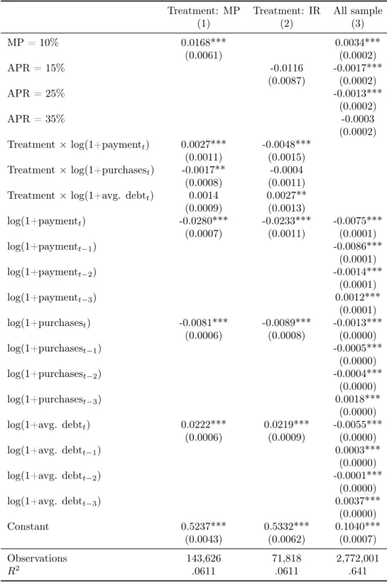
Results are reported in Table 7. Column 1 regresses a dummy variable equal to 1 if

the account ever attrited against the 10MP dummy, and regressor of log purchases, log payments, log debt. In this regression we only use observations for the first month of the experiment as we need a measure of behavior uncontaminated by treatment. Note

that the 10MP dummy is not statistically diﬀerent from zero, and that economically the

coeﬃcient is small, at 0.4% more attrited accounts in the 10MP treatment compared to

the 5MP control. Note also that the interactions of purchases, payment and debt with treatment are quantitatively small: leavers in the 10MP group had 2% less payments, 1% less purchases, and 3% more debt than leavers in the 5MP group at the beginning of the experiment.

Column 2 repeats the analysis for the interest rate treatments, but focusing only on those with 45% and 15% interest. Again the dummy for 15% interest rate is not

significant and interactions with previous behavior economically small. The diﬀerential

attrition due to treatment is quantitatively similar to that of going from 5% to 10% minimum payment.

Finally, Column 3 uses all months and all observations to investigate to what extent

account behavior is diﬀerent a few months before leaving the sample. That it, column

3 is not concerned with diﬀerential eﬀects of treatment on attrition, but rather on the

behavior of stayers versus that of attriters. We use a distributed lag of 3 months to

capture diﬀerences 1 to 3 months before leaving the sample. The semi-elasticities are

tiny for all predictors, less than 0.3%. This means that before leaving accounts that leave the sample are very similar in term of purchases, payments and debts to accounts that stayed.

This analysis gives more credibility to the main findings of the paper. Attrition is unlikely to be driving the results we found.

(16)

7 Conclusions

This paper documents three issues of importance. First, it provides a rare window into bancarization and its perils in a developing country. It shows that the search for credit worthy borrowers is costly since many accounts default and many borrowers leave. Actually net-of-default revenues are not that big. The present discounted value is only 44 pesos on average in the first two years.

Second, it shows that consumer protection for new borrowers in the form of increases in minimum payments does not lead to lower default, but does lead to lower debt and lower bank revenues. Results also show that purchase, payments and debt elasticities are small in the wide range of interest rates we considered. This could mean that the value of credit for these marginal borrowers is large even in the intensive margin. Thirdly, we find no evidence of moral hazard even for this sample of new and risky borrowers as there is no correlation between randomly allocated interest rates and default.

(17)

Tables

Table 1: Summary statistics of key variables

Raw mean Mean given > 0

(1) (2)

Panel A. Demographic characteristics

Age 41.66

-(5.58)

-Sex (male = 1) 0.54

-Marriage status (married = 1) 0.64

-Panel B. Card characteristics (Monthly averages)

Interest paying debt debt 1,152 7,295

(3,571) (5,993) Outstanding balance at the end of the month 5,373 6,056

(5,579) (5,553) Purchases 683.65 1,352.79 (1,755.44) (2,278.71) Payments 845.15 1,076.39 (1,665.88) (1,812.62) Credit Limit 11,690.25 -(9,757.78) -Avg. month-to-month change in credit line 152.92 4,995.67

(2,145) (6,507)

|Avg. month-to-month change in credit line| 340.57 5,457.80 (2,123.19) (6,656.89) Fees incurred 18.32 195.56 (60.65) (67.93) Interest generated 358.59 2,283.06 (1,213.62) (2,232.44) Expected loss 23.06 5,697.94 (444.11) (4,048.82) Revenue 1 468.91 1,302.84 (1,638.96) (1,672.36) Revenue 2 2,246 4,340 (5,135) (4,332)

Panel C. Card characteristics (Proportions)

Cards whose limit change at least once 0.80 -Cards with limit change in a given month 0.10 -Months in which a fee is paid 0.10 0.24 Accounts that pay commissions at least once 0.44 -Months in which interest is paid 0.18 0.33 Accounts in delinquency at least once 0.22 -Accounts in legal default at least once 0.14 -Months in default per account 0.02 0.14

Cancellations 0.22

-Attrition 0.40

-Notes: Standard deviations are shown in parenthesis. Debt, purchases, payments and both revenues are measured in 2007 $MXN. Revenue 1 represents the present value of interests and commissions minus the present value of expected loss. Revenue 2 represents the present value of payments minus the present value of purchases. Delinquency represents the proportion of accounts who did not pay at least one month. Cancellations represents the proportion of accounts cancelled by the end of the sample. Attrition represents the proportion of accounts who disappeared from the sample during the experiment. Mean given>0 stands for the mean given that fees and interests are paid

(18)

Table 2: Interest rate and minimum payment treatments

(a)For each data stratum

Interest Rate Minimum payment Total

10% 5% 15% 2,000 2,000 4,000 25% 2,000 2,000 4,000 35% 2,000 2,000 4,000 45% 2,000 2,000 4,000 Total 8,000 8,000 16,000

Control: 2,000 Full stratum: 18,000

(b)For the full sample

Interest Rate Minimum payment Total

10% 5% 15% 18,000 18,000 36,000 25% 18,000 18,000 36,000 35% 18,000 18,000 36,000 45% 18,000 18,000 36,000 Total 72,000 72,000 144,000

Control: 18,000 Full sample: 164,000

(c)Sample by months of credit card use and cardholder & payment behavior

Months of credit card use Cardholder’s payment behavior Total

Full-balance payer Minimum payer Part-balance payer

6 to 11 months 16,000 16,000 16,000 48,000

12 to 23 months 16,000 16,000 16,000 48,000

24+ months 16,000 16,000 16,000 48,000

Total 48,000 48,000 48,000 144,000

(19)

Ta bl e 3: Base li ne Sum m ar y St at ist ics and Or tho go nal it y -Me ans & St andar d D evi at io ns in Mar ch 20 07 R an do m iz at io n gr ou p [In te re st ra te ⇥ Mi ni m um P ay men t] IR :1 5% IR :2 5% IR :3 5% IR :4 5% Co m pl et e P -V al ue Sa m pl e CTR M P :5 % M P :1 0% M P :5 % M P :1 0% M P :5 % M P :1 0% M P :5 % M P :1 0% sa m pl e si ze (1) (2) (3) (4) (5) (6) (7) (8) (9) (10) (11) (12) P an el A : D em og raphi cs Age 42 42 42 42 42 42 42 42 42 42 0.6666 86,704 (5.58) (5.55) (5.59) (5.59) (5.55) (5.61) (5.60) (5.54) (5.58) (5.58) Pct . of ma les 55 54 55 54 54 54 54 55 54 54 0. 51 61 86 ,7 01 Pct . of ma rr ied 63 65 63 65 64 63 64 63 65 64 0. 13 13 43 ,4 84 P an el B . C ar d char ac te ri st ic s Av er ag e B al an ce 92 7 93 5 91 7 93 8 94 1 96 9 92 2 92 3 95 2 93 6 0.8563 161,590 (3,045) (3,117) (3,061) (3,177) (3,225) (3,240) (3,125) (3,123) (3,233) (3,150) Pur cha ses 58 4 57 9 58 2 59 0 58 6 59 3 60 3 59 3 58 4 58 8 0.9137 161,590 (1,508) (1,500) (1,529) (1,610) (1,573) (1,514) (1,635) (1,622) (1,473) (1,552) Pa ym en ts 81 7 80 3 80 5 81 0 81 3 80 7 83 1 81 1 82 6 81 4 0.7681 161,590 (1,588) (1,537) (1,581) (1,655) (1,625) (1,546) (1,734) (1,642) (1,626) (1,616) Pct . of del inq uen t 1. 39 1. 50 1. 46 1. 44 1. 38 1. 43 1. 59 1. 33 1. 30 1. 43 0. 43 61 16 1, 59 0 N ot es : St an da rd de vi at io ns ar e re po rt ed in pa re nt he si s. Th e p-va lu e in co lu m n (1 1) te st s th e nu ll hy po th es is of al ls tr at a, in cl ud in g th e co nt ro lg ro up (i e. co lu m ns (1 ) to (9 )) ,a re eq ua l. Sa m pl e si ze sh ows th e nu m be r of ob se rv at io ns fo r ea ch va ri ab le in th e fu ll sa m pl e at th e be gi nn in g of th e ex pe ri m en t.

(20)

Table 4: Credit limit diﬀerences by treatment group Credit limit (1) 15%, 5% 24.32 (103.87) 15%, 10% -19.25 (105.14) 25%, 5% -2.06 (103.72) 25%, 10% 80.48 (105.33) 35%, 5% 168.84 (106.27) 35%, 10% 14.85 (104.80) 45%, 5% -13.76 (104.91) 45%, 10% 77.51 (105.37) CTR 11653.52*** (73.82) Observations 3,597,995 R2 _3.5e-05

Notes: Standard errors are reported in parenthesis. This table shows the coeﬃcients of a regression of the credit limit against the treatment dummies using all observations. *, ** and *** represent statistical significance at the 10, 5 and 1 percent, respectively.

(21)

Table 5: Treatment eﬀects for minimum payment and interest rate variations

Debt Purchases Payments Delinquencies Cancelation Default

(1) (2) (3) (4) (5) (6)

Panel A. Short term - April 2008

I:15% P:5% -118** -10.4 -130*** -3.22*** -2.21*** -3.14*** (39.28) (19.63) (18.27) (0.36) (0.30) (0.34) I:15% P:10% -228*** 107*** -21.7 -1.22*** -1.54*** -1.09** (39.42) (19.70) (18.33) (0.36) (0.30) (0.34) I:25% P:5% -32.8 -40.8* -125*** -2.97*** -1.92*** -3.04*** (39.30) (19.64) (18.27) (0.36) (0.30) (0.34) I:25% P:10% -103** 62.9** -22.9 -.661 -1.22*** -.65 (39.43) (19.70) (18.33) (0.36) (0.30) (0.34) I:35% P:5% 139*** -64.6*** -92*** -2.51*** -1.49*** -2.62*** (39.32) (19.65) (18.28) (0.36) (0.30) (0.34) I:35% P:10% -80.8* 32.3 -11 -.728* -.717* -.611 (39.57) (19.77) (18.40) (0.36) (0.30) (0.34) I:45% P:5% 131*** -85.5*** -83.5*** -2.6*** -1.03*** -2.82*** (39.35) (19.66) (18.30) (0.36) (0.30) (0.34) Cons (I:45% P:10%) 1,093*** 686*** 850*** 15*** 9.92*** 13.6*** (27.98) (13.98) (13.01) (0.25) (0.21) (0.24) Observations 118,743 118,743 118,743 144,000 144,000 144,000 R-squared 0.0012 0.0013 0.0010 0.0011 0.0005 0.0014

Panel B. Long term - May 2009

I:15% P:5% 142** -54.5* -143*** -2.82*** -3.63*** -3*** (49.13) (25.55) (22.06) (0.45) (0.35) (0.43) I:15% P:10% -68.4 82.2** -15.4 -1.15** -2.94*** -1.26** (49.64) (25.82) (22.29) (0.45) (0.35) (0.43) I:25% P:5% 255*** -97*** -129*** -2.41*** -3.11*** -2.63*** (49.34) (25.66) (22.16) (0.45) (0.35) (0.43) I:25% P:10% -39.2 -1.96 -33.6 -.65 -2.21*** -.85* (49.78) (25.89) (22.35) (0.45) (0.35) (0.43) I:35% P:5% 376*** -86.2*** -85.3*** -1.08* -2.38*** -1.24** (49.59) (25.79) (22.27) (0.45) (0.35) (0.43) I:35% P:10% 79.2 39 1.45 -.306 -1.27*** -.417 (50.13) (26.07) (22.51) (0.45) (0.35) (0.43) I:45% P:5% 541*** -91.4*** -75.2*** -.733 -1.29*** -1.17** (49.75) (25.88) (22.34) (0.45) (0.35) (0.43) Cons (I:45% P:10%) 1,058*** 743*** 876*** 24.5*** 15*** 22.5*** (35.62) (18.53) (16.00) (0.32) (0.25) (0.30) Observations 87,093 87,093 87,093 144,000 144,000 144,000 R-squared 0.0031 0.0011 0.0011 0.0005 0.0011 0.0006

Notes: Standard errors are reported in parenthesis. *, ** and *** represent statistical significance at the 10, 5 and 1 percent, respectively. The debt, purchases, payments and both revenues are measured in 2007 $MXN. Delinquency and default represents the percentage (from the 144,000 observations) that defaulted their payments at least once prior to the date of the regression. Cancellations represent the percentage of accounts that are cancelled and disappeared from the sample, respectively.

(22)

Table 6: Treatment eﬀects for minimum payment and interest rate variations (Net present value of revenue, measured in March 2007 pesos)

Revenue 1 Revenue 2 (1) (2) I:15% P:5% -458*** -1,776*** (19.56) (52.52) I:15% P:10% -444*** -1,287*** (19.56) (52.52) I:25% P:5% -303*** -1,266*** (19.56) (52.52) I:25% P:10% -293*** -862*** (19.56) (52.52) I:35% P:5% -98.9*** -841*** (19.56) (52.52) I:35% P:10% -161*** -484*** (19.56) (52.52) I:45% P:5% 79.5*** -350*** (19.56) (52.52) Cons (I:45% P:10%) 1,030*** 2,968*** (13.83) (37.14) Observations 144,000 144,000 R-squared 0.0099 0.0116

Notes: Standard errors are reported in parenthesis. *, ** and *** represent statistical significance at the 10, 5 and 1 percent, respectively. The first measure (Revenue 1) calculates for each month interest and fee income and subtracts a rough measure of expected loss of the account if it defaulted, it then calculates the present value using an interest rate of 5 percent for the sample period. The second measure of revenue calculates for each month payments minus purchases, since this is the net flow of income and treats the default as in Revenue 1, and again brings this to the present using a 5 percent rate.

(23)

Table 7: Attrition Results

Treatment: MP Treatment: IR All sample

(1) (2) (3) MP = 10% 0.0168*** 0.0034*** (0.0061) (0.0002) APR = 15% -0.0116 -0.0017*** (0.0087) (0.0002) APR = 25% -0.0013*** (0.0002) APR = 35% -0.0003 (0.0002) Treatment⇥log(1+paymentt) 0.0027*** -0.0048*** (0.0011) (0.0015) Treatment⇥log(1+purchasest) -0.0017** -0.0004 (0.0008) (0.0011)

Treatment⇥log(1+avg. debtt) 0.0014 0.0027**

(0.0009) (0.0013) log(1+paymentt) -0.0280*** -0.0233*** -0.0075*** (0.0007) (0.0011) (0.0001) log(1+paymentt 1) -0.0086*** (0.0001) log(1+paymentt 2) -0.0014*** (0.0001) log(1+paymentt 3) 0.0012*** (0.0001) log(1+purchasest) -0.0081*** -0.0089*** -0.0013*** (0.0006) (0.0008) (0.0000) log(1+purchasest 1) -0.0005*** (0.0000) log(1+purchasest 2) -0.0004*** (0.0000) log(1+purchasest 3) 0.0018*** (0.0000) log(1+avg. debtt) 0.0222*** 0.0219*** -0.0055*** (0.0006) (0.0009) (0.0000) log(1+avg. debtt 1) 0.0003*** (0.0000) log(1+avg. debtt 2) -0.0001*** (0.0000) log(1+avg. debtt 3) 0.0037*** (0.0000) Constant 0.5237*** 0.5332*** 0.1040*** (0.0043) (0.0062) (0.0007) Observations 143,626 71,818 2,772,001 R2 _.0611 _.0611 _.641

Notes: Standard errors are shown in parenthesis. *, ** and *** represent statistical significance at the 10, 5 and 1 percent, respectively. Columns (1) and (2) are regressions where the dependent variable is a dummy indicating those accounts that attrited from the experiment in any moment of time. Column (3) uses as dependent variable attrition att+ 1and uses the full sample through time.

(24)

Figures

Figure 1: Number of credit cards in Mexico

.02 .04 .06 .08 .1 .12 Pro po rt io n 5 10 15 20 25 # C re di t C ard s (Mi lli on s)

Jan/02 Jan/04 Jan/06 Jan/08 Jan/10 Jan/12 Number of credit cards [Left]

Loan portfolio: Non performing / Total [Right]

Source: Banco de México

Figure 2: Credit cards are the main bancarization instrument

(a)Growth in CC holdings by income decile

(2004-2010) 0 50 100 150 200 250 G ro w th +(% ) 0 2 4 6 8 10 Income+decile

(b)Entry into formal credit by type of loan

(2011) 0 20 40 60 Pe rce nt ag e (% )

Auto Bank Dept. stores Other Personal/Payroll Phone

All New clients

(25)

Figure 3: Timeline for the experiment

Dec/2006 • Randomization of interest rate and minimum payment groups Mar/2007 • Experiment starts

Apr/2008 • First results shown (medium-term)

May/2009 • Experiment ends and second results shown (long-term)

Figure 4: Payment / Current amount due at the beginning of the experiment

18.1 0.2& 0.5& 1.5& 4.2& 13.6 5.3&

4.2& 3.7& 3.8& 3.6&

2.8& 2.3& 2.0& 1.8&_{1.5& 1.4& 1.2& 1.1& 1.0&} 25.9 Mo re &th an &2 0% 18.3% 24.5% 55.1% 0 5 10 15 20 25 Pe rc en tag e& of &ac co un ts &(% ) 0 .05 .1 .15 .2 Payment&/&Amount&due

(26)

Figure 5: Histogram - Revenue by default (a)Revenue 1 0 .2 .4 .6 .8 F ra ct io n of co nsu me rs -10,000 -5,000 0 5,000 10,000 Profit (MXN)

Defaulted at least once Never defaulted

(b) Revenue 2 0 .1 .2 .3 F ra ct io n of co nsu me rs -50,000 0 50,000 Profit (MXN)

Defaulted at least once Never defaulted

Note: Revenue 1 represents the present value of interests and commissions minus the present value of expected loss. Revenue 2 represents the present value of payments minus the present value of purchases. Within each histogram, the null hypothesis of both groups having the same distribution is rejected using a Kolmogorov-Smirnov test (p-value

(27)

Figure 6: Minimum payment variations: Results

(a)Average Balance

900 1000 11 00 1200 1300 1400 A ve ra ge b al an ce (MXN )

Jan/07 Jul/07 Jan/08 Jul/08 Jan/09 Jul/09 MP: 5% MP: 10% (b)Purchases 400 600 800 1000 1200 Pu rch ase s (MXN )

Jan/07 Jul/07 Jan/08 Jul/08 Jan/09 Jul/09 MP: 5% MP: 10% (c) Payments 700 800 900 1000 11 00 Pa yme nt s (MXN )

Jan/07 Jul/07 Jan/08 Jul/08 Jan/09 Jul/09 MP: 5% MP: 10%

(d)Accounts (%) with positive average

balance 12 14 16 18 20 Acco un ts (% )

Jan/07 Jul/07 Jan/08 Jul/08 Jan/09 Jul/09

MP: 5% 10%

(28)

Figure 6: Minimum payment variations: Results (2)

(e)Accounts in delinquency at least once

0 5 10 15 20 Acco un ts (% )

Jan/07 Jul/07 Jan/08 Jul/08 Jan/09 Jul/09 MP: 5% MP: 10% (f) Cancelled accounts 0 5 10 15 20 25 Acco un ts (% )

Jan/07 Jul/07 Jan/08 Jul/08 Jan/09 Jul/09 MP: 5% MP: 10% (g)Accounts in delinquency 0 2 4 6 8 10 Acco un ts (% )

MP: 5% 10%

(h)Accounts with late payments

2 4 6 8 10 Acco un ts (% )

MP: 5% 10%

(i)Sample attrition

0 1 2 3 4 % Pe op le

Jan/07 Jul/07 Jan/08 Jul/08 Jan/09 Jul/09 MP: MP: 5% MP: 10% CTR

(29)

Figure 7: Annual percentage rate variations: Results

(a)Average Balance

900 1000 11 00 1200 1300 A ve ra ge b al an ce (MXN )

APR: 15% 25% 35% 45% (b)Purchases 400 600 800 1000 Pu rch ase s (MXN )

Jan/07 Jul/07 Jan/08 Jul/08 Jan/09 Jul/09 APR: 15% 25% 35% 45% (c) Payments 700 800 900 1000 11 00 Pa yme nt s (MXN )

APR: 15% 25% 35% 45%

(d)Accounts (%) with positive average

balance 12 14 16 18 Acco un ts (% )

Jan/07 Jul/07 Jan/08 Jul/08 Jan/09 Jul/09 APR: 15% 25% 35% 45%

(30)

Figure 7: Annual percentage rate variations: Results (2)

(e)Accounts in delinquency at least once

0 5 10 15 20 25 Acco un ts (% )

Jan/07 Jul/07 Jan/08 Jul/08 Jan/09 Jul/09 APR: 15% 25% 35% 45% (f) Cancelled accounts 0 5 10 15 20 25 Acco un ts (% )

Jan/07 Jul/07 Jan/08 Jul/08 Jan/09 Jul/09 APR: 15% 25% 35% 45% (g)Accounts in delinquency 0 5 10 Acco un ts (% )

(h)Accounts with late payments

2 4 6 8 10 Acco un ts (% )

(i)Sample attrition

0 1 2 3 4 % Pe op le

Jan/07 Jul/07 Jan/08 Jul/08 Jan/09 Jul/09 APR: 15% 25% 35% 45% CTR

(31)

Figure 8: Predicted credit limit depending on default ← ← 9,000 10,500 12,000 13,500 Cr ed it. lim it. (MXN )

Jan/07 Jul/07 Jan/08 Jul/08 Jan/09

Defaults: never 3rd.m 3rd.&.6th.m

Note: These lines represent what would happen if an account happens to be delinquent in the first 3 months (red dashed line) or happens to be delinquent in the first 6 months (green dotted line). For comparison, the blue solid line represents the credit limit of an account that never defaults. The lines are plotted from a regression of credit limit against time dummies, number of delinquencies dummies and number of default dummies.

(32)

References

Adams, William, Liran Einav, and Jonathan Levin.2009. “Liquidity
Constraints and Imperfect Information in Subprime Lending.” The American
Economic Review, 99(1): pp. 49–84.
Dehejia, Rajeev, Heather Montgomery, and Jonathan Morduch. 2012. “Do
interest rates matter? Credit demand in the Dhaka slums.” Journal of
Development Economics, 97(2): 437 – 449.
Einav, Liran, Mark Jenkins, and Jonathan Levin. 2013. “The impact of credit
scoring on consumer lending.” The RAND Journal of Economics, 44(2): 249–274.
Gross, David B., and Nicholas S. Souleles.2002. “Do Liquidity Constraints and
Interest Rates Matter for Consumer Behavior? Evidence from Credit Card
Data.” Quarterly Journal of Economics, 117(1): 149–185.
Karlan, D., and J. Zinman. 2008. “Credit Elasticities in Less-Developed
Economies: Implications for Microfinance.” American Economic Review,
98(3): 1040–1068.
Karlan, Dean, and Jonathan Zinman.2009. “Observing Unobservables:
Identifying Information Asymmetries with a Consumer Credit Field
Experiment.” Econometrica, 77(6): pp. 1993–2008.
Laibson, David, Andrea Repetto, and Jeremy Tobacman. 2003. “A Debt
Puzzle.” In Knowledge, Information, and Expectations in Modern Economics: In
Honor of Edmund S. Phelps. , ed. Philippe Aghion, Roman Frydman, Joseph Stiglitz and Michael Woodford. Princeton University Press.
Meier, Stephan, and Charles Sprenger. 2010. “Present-Biased Preferences and
Credit Card Borrowing.” American Economic Journal: Applied Economics,
2(1): 193–210.
Smale, Pauline. 2005. “Credit Card Minimum Payments: RS22352.” Congressional
Research Service: Report, 1.
Stewart, Neil. 2009. “The Cost of Anchoring on Credit-Card Minimum